Edgar José Sanches Mascarenhas

(1)

Edgar José Sanches Mascarenhas

Licenciatura em Ciências da Engenharia Biomédica

Mechanical characterization of aortas using

2D ultrasound elastography

Dissertação para obtenção do Grau de Mestre em Engenharia Biomédica

Júri:

Presidente: Prof. Doutora Carla Maria Quintão Pereira

Arguente: Prof. Doutor Mário António Basto Forjaz Secca

Vogal: Prof. Doutor Pedro Manuel Cardoso Vieira

Outubro 2014

Orientadores: Richard Loptata, Professor Auxiliar, Technische

Universiteit Eindhoven, Holanda

Mathijs Peters, M.Sc., Technische Universiteit

Eindhoven, Holanda

Co-orientador: Pedro Vieira, Professor Auxiliar, FCT-UNL

Orientadores: Richard Loptata, Professor Auxiliar, Technische

Universiteit Eindhoven, Holanda

Mathijs Peters, M.Sc., Technische Universiteit

Eindhoven, Holanda

(2)

ii

(3)

iii

Mechanical characterization of aortas using 2D ultrasound elastography

Universidade Nova de Lisboa.

A Faculdade de Ciências e Tecnologia e a Universidade Nova de Lisboa têm o direito, perpétuo

e sem limites geográficos, de arquivar e publicar esta dissertação através de exemplares impressos

reproduzidos em papel ou de forma digital, ou por qualquer outro meio conhecido ou que venha

a ser inventado, e de a divulgar através de repositórios científicos e de admitir a sua cópia e

distribuição com objetivos educacionais ou de investigação, não comerciais, desde que seja dado

(4)

(5)

v

Acknowledgments

First, I would like to thank Professor Frans van de Vosse for welcoming me in the Cardiovascular

Biomechanics Group at Technische Universiteit Eindhoven (TU/e), and giving this great

opportunity of doing my master thesis in his research group.

Secondly, a deep and meaningful thanks to my supervisor Richard Lopata, for believing in my

work and being always present, while giving me the freedom to build my own path at the same

time. Richard, I will always be grateful for your guidance during these seven months. With you I

learnt not only scientific method, but far beyond the books and conventional.

I would also like to thank my daily supervisor Mathijs Peters for the assistance during the

development of this thesis, in particular with laboratory procedures. Mathijs, thank you for all the

support, without pre-scheduling meetings or formalities since the first day.

I kindly thank Professor Mário Forjaz Secca for supporting me in establishing the required

agreement between both universities.

A word to Professor Pedro Vieira for remaining my link to FCT-UNL and for the help provided

during the seven months abroad.

I also want to express my gratitude to all Master students at TU/e who worked by my side and

to the Dispuut 3004 – TU/e Materials Technology Student Association. This was a remarkable experience, and part of it was also due to the friends from around the world that gathered for the

Spring semester at TU/e in 2014.

To all my friends in Portugal with whom I shared this journey on the last five years, Rui Dinis,

Bruno Ribeiro, João Tavares, Artur Gonçalves, Manuel Coelho, Alexandre Medina, Ana Isabel

Sousa, Luísa Fialho, Andreia Serrano, Inês Ropio and Joana Costa, you have made this 5-year

journey more fun and pleasant.

Finally, a special thanks to my family, my parents and my sister for their unconditional support

(6)

(7)

vii

Abstract

Rupture of aortic aneurysms (AA) is a major cause of death in the Western world. Currently,

clinical decision upon surgical intervention is based on the diameter of the aneurysm. However,

this method is not fully adequate. Noninvasive assessment of the elastic properties of the arterial

wall can be a better predictor for AA growth and rupture risk.

The purpose of this study is to estimate mechanical properties of the aortic wall using in vitro inflation testing and 2D ultrasound (US) elastography, and investigate the performance of the

proposed methodology for physiological conditions.

Two different inflation experiments were performed on twelve porcine aortas: 1) a static

experiment for a large pressure range (0 – 140 mmHg); 2) a dynamic experiment closely

mimicking the in vivo hemodynamics at physiological pressures (70 – 130 mmHg). 2D raw radiofrequency (RF) US datasets were acquired for one longitudinal and two cross-sectional

imaging planes, for both experiments. The RF-data were manually segmented and a 2D vessel wall displacement tracking algorithm was applied to obtain the aortic diameter–time behavior. The shear modulus G was estimated assuming a Neo-Hookean material model. In addition, an incremental study based on the static data was performed to: 1) investigate the changes in G for increasing mean arterial pressure (MAP), for a certain pressure difference (30, 40, 50 and 60

mmHg); 2) compare the results with those from the dynamic experiment, for the same pressure

range.

The resulting shear modulus G was 94 ± 16 kPa for the static experiment, which is in agreement with literature. A linear dependency on MAP was found for G, yet the effect of the pressure difference was negligible. The dynamic data revealed a G of 250 ± 20 kPa. For the same pressure range, the incremental shear modulus (Ginc) was 240 ± 39 kPa, which is in agreement

with the former. In general, for all experiments, no significant differences in the values of G were found between different image planes.

This study shows that 2D US elastography of aortas during inflation testing is feasible under

controlled and physiological circumstances. In future studies, the in vivo, dynamic experiment should be repeated for a range of MAPs and pathological vessels should be examined.

Furthermore, the use of more complex material models needs to be considered to describe the

(8)

viii

Key-words: aortic aneurysm, vascular biomechanics, inflation testing, 2D ultrasound

(9)

ix

Resumo

A rutura de aneurismas da aorta (AA) é das principais causas de morte no mundo ocidental.

Atualmente, a decisão clínica sobre a realização de uma intervenção cirúrgica é baseada no

diâmetro do aneurisma. Contudo, este método não é o mais adequado. A avaliação não invasiva

das propriedades elásticas da parede da artéria poderá ser um melhor indicador na previsão do

crescimento e risco de rutura do AA.

O objetivo deste estudo é determinar as propriedades mecânicas da parede da aorta, recorrendo

a experiências de pressurização in vitro e a elastografia 2D por ultrassom (US), e investigar o desempenho da metodologia proposta sob condições fisiológicas.

Duas experiências de pressurização foram executadas em doze aortas de porco: 1) uma experiência ‘estática’, considerando um intervalo significativo de pressão (0 - 140 mmHg); 2) uma experiência ‘dinâmica’, simulando as condições hemodinâmicas presentes in vivo a pressões fisiológicas (70 – 130 mmHg). Para ambas as experiências, conjuntos de dados 2D de

radiofrequência (RF) foram adquiridos para um plano de imagem longitudinal e duas secções

transversais. Os dados de RF foram segmentados manualmente e um algoritmo 2D de

monitorização do deslocamento da parede da artéria foi aplicado com o intuito de obter o diâmetro

da aorta em função do tempo. O shear modulus G foi estimado assumindo um modelo de material Neo-Hookeneano. Além disso, um estudo ‘incremental’ baseado nos dados da experiência ‘estática’ foi realizado com o propósito de 1) investigar as mudanças nos valores de G no caso de aumento na pressão arterial média (PAM), para uma determinada diferença de pressão (30, 40, 50 e 60 mmHg); 2) comparar os resultados com os da experiência ‘dinâmica’, considerando o mesmo intervalo de pressão.

No caso da experiência ‘estática’, o valor de G resultante foi de 94 ± 16 kPa, o que está de acordo com a literatura. Foi observada uma dependência linear entre os valores de G e PAM, contudo o efeito da diferença da pressão revelou-se negligível. Os resultados da experiência ‘dinâmica’ revelaram um valor de G de 250 ± 20 kPa. Para o mesmo intervalo de pressão, o shear modulus incremental (Ginc) foi de 240 ± 39 kPa, estando em concordância com o anterior. No

geral, para todas as experiências, não foram verificadas diferenças significativas nos valores de

(10)

x

Este estudo demonstra que o método de elastografia 2D por US em aortas durante experiências

de pressurização é viável sob circunstâncias controláveis e fisiológicas. Em estudos futuros, a experiência ‘dinâmica’ poderá ser repetida para um intervalo de PAMs e poderão ser analisadas artérias patológicas. Além disso, a utilização de modelos mais complexos necessita de ser

considerada a fim de se obter uma descrição do comportamento não-linear do tecido vascular.

Key-words: aneurisma da aorta, biomecânica vascular, experiências de pressurização,

(11)

xi

List of Figures

Figure 2.1 – Normal (healthy) aorta anatomy (left) and abdominal aortic aneurysm anatomy (right) (Speelman, 2009). ... 8

Figure 2.2 – Proposed size-dependent clinical management for asymptomatic abdominal aortic aneurysms (Sakalihasan et al., 2005). ... 9

Figure 2.3 – AAA open surgical repair (a) and AAA endovascular repair (b) (Callanan et al., 2011). ... 10

www.adamimages.com). ... 11

Figure 2.5 – Stress-strain curve for the aorta and the elastin and collagen curves (Raghavan et al., 1996)... 14

Figure 2.6 – Schematic view of the aorta. The pulsating blood pressure yields strains in the circumferential (εcirc), radial (εrad) and longitudinal (εlong) directions (Peters, 2013). ... 14

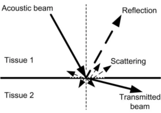
Figure 2.7 - Schematic representation of the reflection and scattering of acoustic waves in

tissue (Lopata, 2010). ... 19

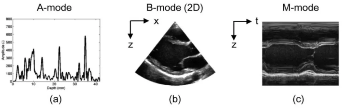
Figure 2.8 - Some of the different types of US acquisition modes: (a) A-mode, a single echo

line; (b) B-mode, an image created by several neighboring echo lines; (c) M-mode, time-series of

a single echo line (Lopata, 2010). ... 20

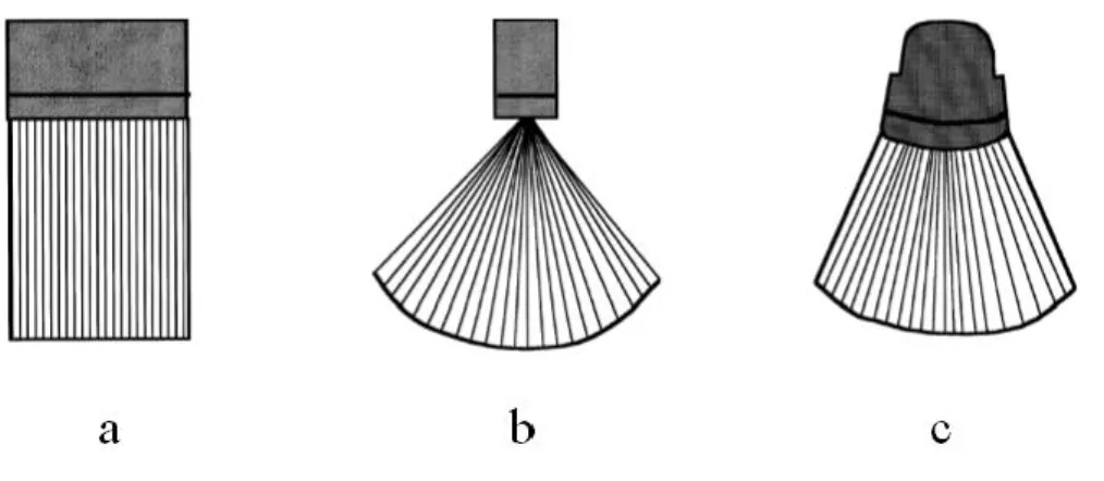
Figure 2.9 – Types of US transducers: linear-array transducer (a), phased-array transducer (b), curved-array transducer (c). ... 23

Figure 2.10 – A single RF-line of a time frame i (a) and the RF-line of the next time frame i+1 (b). c) The light grey line represents the auto-correlation of RF-line (a) and the black line

corresponds to the cross-correlation of RF-lines (a) and (b). The shift of the cross-correlation

function with respect to the auto-correlation function illustrated in the figure corresponds to the

(14)

xiv

Figure 2.11 – Schematic representation of 2D B-mode speckle tracking. A small segment of image in time frame 1 (red square) is matched with a search area (green square) in the next time

frame 2. (Lopata, 2010). ... 25

Figure 3.1 – A defrosted aorta with closed side-branches. Side branches were closed with

thread. In the case the side branch was too short to close with thread, superglue was used to close

the side branch. ... 30

Figure 3.2 – The leakage test. First, the aorta was closed at the distal end and connected to a syringe at the proximal end. Next, the aortic segment was inflated by adding water via the syringe

so that any possible leakages could then become visible. The leakages were marked using a

marker pen. Finally, these leakages were closed using superglue. This procedure was repeated

until there were no leakages left. ... 30

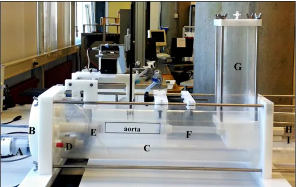
Figure 3.3 – The experimental setup. The axial piston pump (A) pushes the water from the

circular compartment (B) towards the aorta, which is placed inside the water tank (C). A

mechanical valve (D) is used to allow water to flow from the water tank back to the circular

compartment but not vice versa. The proximal end (larger end) of the aorta is connected to another mechanical valve, i.e., ‘aortic valve’ (E), and the distal end (smaller end) to the silicon tube (F). This silicon tube is attached to a vertical air column (G) with two associated resistances (upper

and lower resistance, H and I, respectively). ... 31

Figure 3.4 – The 3-element Windkessel model. C1represents the aortic compliance, Z1 the

peripheral resistance and Z0 the characteristic impedance of the proximal end of the aorta (input

impedance of the circuit). ... 32

Figure 3.5 – The vertical air column (G) which can be filled with water and the two associated resistances (upper and lower resistances, H and I, respectively) zoomed in. Both resistances can

be used to control the water level inside the air column. H is used to control the water inflow from

the silicon tube into the air column, whereas I is used to determine the water flow from the air

column into the water tank. ... 33

Figure 3.6 – Schematic overview of the two separate loops used for heating the water inside the water tank. The first loop (dark blue) contains salt water; a roller pump is used to push the

water from the water tank into the heat exchanger, where it gets heated by the hot tap water that

flows in its surroundings; then, the salt water returns to the water tank. The tap water circulates

in a separate second loop (light blue) which connects the heating circulator to the heat exchanger.

(15)

xv

Figure 3.7 - The pre-stretch device used to apply the physiological longitudinal pre-stretch.

The two-headed black arrow indicates the direction in which the distance between the two

connectors attached to the aorta was increased to apply a pre-stretch in the longitudinal direction.

... 36

Figure 3.8 - Pressure signal obtained during the static experiment. ... 37

Figure 3.9 – The cylindrical iron bar is pushed to the right for the static experiment, preventing the aortic valve from closing and thus allowing for a complete deflation of the aortic segment. 37

Figure 3.10 – The physiological pressure signal (Klabunde, 2005). ... 38

Figure 3.11 – Pressure signal obtained during the dynamic experiment... 38

Figure 3.12 – Positioning the US probe in the setup (position for cross-sectional view). ... 39

Figure 3.13 – US-Scanner used in the experiments (MyLab 70 US scanner, Esaote© Europe, Maastricht, NL). ... 40

Figure 3.14 – Schematic overview of the interaction between the main components of the

devised laboratory setup: the axial piston pump, the water tank, the air column, the US probe, the

PC workstation and the US-scanner with the associated ArtLAB© system. P (in red in this figure)

represents the pressure sensor. During the US-acquisition, the pressure signal and the raw

RF-data are automatically saved in the ArtLAB© system. ... 41

Figure 3.15 – Example of longitudinal (left) and cross-sectional (right) B-mode US images obtained. ... 41

Figure 3.16 – Schematic overview of the US acquisition within the aortic segment. In this

figure, as an example, one longitudinal B-mode US image is acquired between the second and the

fourth side branch of the aorta. Next, cross-sectional B-mode US images are acquired between

the second and third side branches (cross-section 1) and between the third and fourth side branches

(cross-section 2). The numbers 1-5 (in red) indicate the side branches. ... 42

Figure 3.17 – Schematic overview of the 6 different US data sets acquired for each aorta. .. 42

Figure 3.18 - Example of a manual inner wall segmentation performed in a US cross-sectional

image. The red points represent aortic inner wall points (manual segmentation). The blue points

are defined in the outward direction, i.e., in the normal direction of the red circle, defining the

(16)

xvi

Figure 3.19 – Example of pressure and diameter curves before (left) and after (right)

synchronization is performed. The red curve represents diameter data, whereas the blue curve

represents pressure data. It should be noted that both curves were normalized with respect to their

respective maximum values. The horizontal axis corresponds to the number of frames. ... 45

Figure 3.20 – The vessel visualized as a flat strip with the corresponding radial (x-direction), circumferential (y-direction) and longitudinal (z-direction) directions... 46

Figure 3.21 - The two steps of the US-experiments: first, the aorta is subject to a longitudinal

pre-stretch of 1.22 (F0) and then to an increasing hydrostatic pressure (F1). It should be noted that

the circles illustrated in the figure represent cross-sectional views of the aorta. ... 47

Figure 3.22 – Example of a static pressure-diameter curve (in red) obtained. The region of the plot between the black dashed lines represent the respective dynamic pressure range (ΔPdyn). The dynamic pressure range (ΔPdyn) is defined as the difference between the systolic pressure (Psys) and the diastolic pressure (Pdia). ... 52

Figure 4.1 – Plot with the stress-strain curves of the different static US-experiments performed in aorta 2. The red curve corresponds to the US longitudinal view, the blue curve to the US

cross-sectional view no. 1 and the green curve to the US cross-cross-sectional view no.2. Stress actually refers

to the circumferential stress [kPa], whereas strain refers to the Finger strain (dimensionless). . 57

Figure 4.2 – Plot with the values of shear modulus for the twelve aortas obtained from the analysis of static US data sets in the longitudinal view (red squares), cross-section 1 (blue

triangles), and cross- section 2 (green circles). The overall mean value of G (black solid line) and the overall mean ± standard deviation are also shown (black dashed lines). The overall mean G was 94 ± 16 kPa. ... 57

Figure 4.3 - Plot with the dynamic values of shear modulus for all aortas, obtained in the

longitudinal view (red squares), cross-section 1 (blue triangles) and cross-section 2 (green

circles). The overall mean value of G (black solid line) and the overall mean ± standard deviation are also shown (black dashed lines). The overall mean G was 250 ± 20 kPa. ... 59

Figure 4.4 - The incremental shear modulus as a function of mean arterial pressure (MAP) for a pulse pressure ΔP of, respectively, 30 mmHg (a), 40 mmHg (b), 50 mmHg (c), and 60 mmHg (d). The red lines indicate the longitudinal view, the green lines correspond to cross-section 1 and

the blue lines correspond to cross-section 2. The error-bars indicate the standard deviation of the

(17)

xvii

Figure 4.5 - Plot with the values of incremental shear modulus (Ginc) for all aortas and all US

image views: the longitudinal view (red squares), section 1 (blue triangles) and

cross-section 2 (green circles). The overall mean value of Ginc (black solid line) and the overall mean ± standard deviation (black dashed lines) are also shown. The overall mean incremental shear

modulus was 240 ± 39 kPa. ... 61

Figure 4.6 – Scatter plot with the correspondence between the values of incremental shear modulus (Ginc) and the respective values of dynamic shear modulus (Gdyn) considering the same

US image view. The red squares correspond to longitudinal view, the blue triangles to

cross-section 1 and the green circles to cross-cross-section 2. ... 62

Figure 4.7 – A Bland-Altman plot to compare the values of G obtained using two different

methods: the dynamic US-experiment and the incremental analysis. The red squares correspond

to longitudinal view, the blue triangles to cross-section 1 and the green circles to cross-section 2.

The mean difference in G, i.e., the bias (black solid line) and the mean difference in G ± 1.96

times the standard deviation, the so-called limits of agreement (black dashed lines) are shown as

well. ... 63

Figure 5.1 - Positioning of the US probe for acquiring longitudinal US images. Situation A

(left) shows the correct positioning of the US probe, whereas situation B (right) shows the US

probe not perfectly placed. Situation B will lead to an underestimation of the diameter. A similar

(18)

(19)

xix

List of Tables

Table 2.1 – Composition of normal (healthy) aortic tissue and AAAs (He et al., 1994). ... 15

Table 4.1 – Initial length (L0) [cm] measured for each aorta and the respective resulting length

after applying the 22% of longitudinal pre-stretch [cm]. ... 55

Table 4.2 – The resulting initial wall thickness (h0) [mm] of the twelve porcine aortas obtained

from the analysis of the static US data sets. ... 56

Table 4.3 – Diameter range (ΔD) [mm], pressure range (ΔP) [mmHg], initial wall thickness (h0) [mm] and the respective value for shear modulus (G) [kPa] regarding aorta 2 static US data

sets. ... 56

Table 4.4 – The resulting initial wall thickness (h0) of the twelve porcine aortas obtained from

the analysis of the dynamic US data sets. ... 58

Table 4.5 - Diameter range (ΔD) [mm], pressure range (ΔP) [mmHg], initial wall thickness

(h0) [mm] and the respective value of shear modulus (G) [kPa] for aorta 2. ... 59

Table 4.6 – Original pressure and diameter arrays (ΔP and ΔD, respectively) obtained from aorta 8 static US data sets. The pressure and diameter arrays corresponding to the dynamic range

(ΔPdynand ΔDdyn, respectively) plus the wall thickness at the diastolic pressure (hPdia) (columns in

(20)

(21)

xxi

Acronyms

AA: Aortic aneurysm

AAA: Abdominal Aortic Aneurysm

BNC Connector: Bayonet Neill-Concelman Connector

CCF: Cross-Correlation Function

COPD: Chronic Obstructive Pulmonary Disease

CPU: Central Processing Unit

CT: Computed Tomography

CVD: Cardiovascular Disease

EVAR: Endovascular Repair

FEA: Finite Element Analysis

FOV: Field of View

GUI: Graphical User Interface

ILT: Intraluminal Thrombus

IVUS: Intravascular Ultrasound

MAP: Mean Arterial Pressure

MRI: Magnetic Resonance Imaging

PBS-solution: Phosphate Buffered Saline solution

RF: Radiofrequency

ROI: Region of Interest

SMC: Smooth Muscle Cells

SNR: Signal-to-Noise Ratio

(22)

(23)

1

1. Introduction

1.1 Motivation

In this day and age, cardiovascular disease (CVD) is the leading cause of deaths worldwide. An

estimated 17.3 million people died in 2008, representing 30% of all global deaths (Mendis et al.,

2011). A sub-group of patients suffer from a thoracic, abdominal or even cerebral aneurysm.

In particular, an abdominal aortic aneurysm (AAA) is a permanent local dilatation of the aorta

in the abdominal cavity of more than 50% of its original diameter (Zankl et al., 2007). The

incidence of this condition is growing due to general aging of population and an increase in the

amount of screening programs (Lederle et al., 1997), with approximately 150.000 new cases being

diagnosed every year (Bengtsson et al., 1996). If left untreated, AAA will increase in size, until

it eventually ruptures, causing a life-threatening hemorrhage. Of the patients with an AAA, 75%

remain symptom free until AAA rupture occurs, which is fatal in most cases (Zankl et al., 2007).

Annually, 15.000 to 20.000 deaths occur in the United States due to AAA rupture (Bush et al.,

2003) and, as a result, remains the 13th_{most common cause of death in that country (Wilmink et}

al., 1998).

In order to determine if an AAA requires surgical intervention, the risk of rupture should be

carefully assessed and balanced against the risk associated with the surgical repair. Currently, the

decision to electively repair an AAA is based on the maximum anterior-posterior diameter of the

aneurysm, i.e., when the maximum anterior-posterior diameter of the aneurysm is larger than

5-5.5 cm it is thought that the risk of rupture is high (Greenhalgh et al., 1998; Zankl et al., 2007).

(24)

1. INTRODUCTION

2

AAA rupture, since several studies have shown that small aneurysms, i.e., below 5.5 cm, can

rupture (Choksy et al., 1999; Nicholls et al., 1998), while stable AAAs considered large, i.e.,

above 5.5 cm, do not rupture, given the life expectancy of the patient (Darling et al., 1977;

Conway et al., 2001). Hence, intervention based on the maximum diameter criterion can be

performed too late, prematurely or even subject patients to unnecessary surgical risks.

Besides maximum diameter, AAA growth rate can also be taken into consideration in the

decision for AAA repair. Yet, previous studies have shown large variations in growth rate

between AAAs and discontinuous growth was observed (Kurvers et al., 2004).

Both these criteria should be replaced by a more patient-specific criterion to better predict the

likelihood of AAA rupture. In general, such a solution is sought for in the field of biomechanics.

As a result, AAA wall stress analyses have been introduced (Raghavan et al., 2000; Fillinger et

al. 2002). The basic principle of this approach is that when the stress in the AAA wall locally

exceeds the strength of the wall, AAA rupture occurs. A thorough analysis on biomechanical

properties of AAAs such as wall strength, elasticity or aortic compliance (Vorp et al., 1996; Imura

et al., 1986; Long et al., 2004) can give a better understanding on AAA biomechanical behavior

and, thus, a more accurate prediction of AAA growth and rupture. Elasticity can be assessed by

destructive testing, but also non-invasively by means of ultrasound (US) elastography (Lopata et

al., 2014).

This study intends to develop an accurate and reproducible method for the mechanical

characterization of aortas by determining and analyzing biomechanical properties of the aortic

wall, such as the shear modulus G, using in vitro inflation testing and 2D US elastography. The performance of this method was also investigated for physiological conditions. Ultimately, the

goal is to provide a non-invasive tool based on in vivo US imaging and biomechanical patient-specific analysis, with the purpose of helping clinicians to detect and monitor weakening of the

aortic wall, which may lead to an improvement of AAA growth prediction, and an optimization

of both the follow-up plan and the moment of aortic surgical repair. In this sense, this approach

may have the potential to serve as an accurate and robust method to improve AAA risk

(25)

1. INTRODUCTION

3

1.2 State of the art

Current widespread clinical thinking is that AAA rupture is best predicted by monitoring its

maximum diameter; i.e., it is conventionally accepted that the risk of rupture is highest when the

maximum anterior-posterior AAA diameter reaches 5.5 cm (Greenhalgh et al., 1998). However,

from previous research it becomes clear that the maximum AAA diameter in some cases

underestimates the risk of rupture (Choksy et al., 1999; Nicholls et al., 1998), leading to

unexpected ruptures, whereas in other cases the risk is overestimated (Darling et al., 1977;

Conway et al., 2001). In the latter case, AAA may be unnecessarily repaired, with all associated

surgical risks. Hence, additional indicators are required to provide a more accurate and robust

assessment of AAA growth and rupture, based on a more patient-specific approach.

From a biomechanical perspective, rupture of AAA occurs when wall stress locally surpasses

wall strength. The Law of Laplace states that wall stress in a thin-walled cylinder increases

linearly with increasing diameter and transmural pressure, and decreases for increasing wall

thickness. In this way, the Law of Laplace is regarded as the theoretical framework for using the “maximum diameter criterion” for potential AAA rupture prediction (Hall et al. 2000), since it states that the stress on the AAA wall is proportional to its diameter. However, the stresses acting

on an AAA wall are not evenly distributed and are highly dependent on the shape (e.g. profile,

tortuosity) of the specific AAA (Vorp et al., 1998).

Over the past two decades, several research groups have been suggesting patient-specific wall

stress analyses as a potential predictor of AAA rupture, based on Finite Element Analysis (FEA)

(Fillinger et al., 2002; Truijers et al., 2007; Raghavan et al., 2000; Speelman et al., 2010). Fillinger

et al. (2002) found that the peak wall stress for ruptured and symptomatic AAAs was significantly

higher than that for electively repaired AAAs. In another study conducted by this same group, it

was shown that the peak wall stress is a better predictor of AAA rupture than the maximum AAA

diameter (Fillinger et al., 2003). Likewise, a more recent study found similar results, showing a

high correlation between the AAA rupture and the location of the peak wall stress

(Venkatasubramaniam et al., 2004). Moreover, in a study of Speelman et al. (2010) it was

observed that relatively low AAA wall stress is associated with lower AAA growth rate, but no

significant correlation was found between absolute or relative wall stress analysis and AAA

biomarker concentrations. In all aforementioned studies, patient-specific AAA geometries were

(26)

1. INTRODUCTION

4

In order to monitor and assess AAA wall growth in a clinical environment, follow-up

surveillance on a regular basis is required. In this sense, CT imaging is not adequate, considering

the use of ionizing radiation and lack of patient-specific input apart from geometry. Alternatively,

MRI (Magnetic Resonance Imaging) is often used to examine AAAs, owing its good image

quality (Lee et al., 1984). One example is the study of Kramer et al. (2004) where T1 and

T2-weighted spin echo imaging was performed in 23 AAA patients in order to detect atherosclerotic

plaque components in AAAs. The study reports that higher signal on T2-weigthed MRI provides

an accurate identification of the fibrous cap and thrombus within an AAA. Nonetheless, MRI is

very time-consuming and expensive. Besides, contrast agents may be needed to enhance image

quality and to acquire dynamic MRI scans.

Ultrasound (US) imaging combines its non-invasive nature, the absence of radiation hazard

and its high temporal resolution. US imaging represents the modality of choice for AAA

detection, initial assessment and follow-up surveillance, with a sensitivity of 95% and a specificity

of almost 100% (Lindholt et al., 1999). The accuracy of size measurements using US is especially

important to reliably monitor AAA growth. Singh et al. (1998) reported intra- and inter-observer

variability in US measurements of AAA diameter less than 4 mm and concluded that the

maximum AAA diameter could be measured using US imaging with a high degree of accuracy.

The high temporal resolution of US imaging enables a comprehensive study of the dynamical

behavior of the aneurysm when exposed to blood pulse, providing an accurate assessment of

patient-specific parameters, such as distensibility, tissue deformation (i.e., strain) or aortic

compliance, which can be used to improve FEA or used as indicators of aneurysm growth. Several

authors have used ultrasound to estimate the mechanical properties of AAA by tracking the

dynamical change in diameter due to the passing blood pulse (Imura et al., 1986; Long et al.,

2004; Wilson et al, 2003). The changing diameter is used to achieve a measure of strain. This

approach provides information about the dilation of the aorta as function of time and space along

the segment of the aorta. Imura et al. (1986) presented a method using B-mode US imaging for

tracking the dynamic diameter of the abdominal aorta over the cardiac cycle in order to assess

elastic properties of human abdominal aorta in vivo. Wilson et al. (1999) used US diameter

tracking to report that large aneurysms tend to be stiffer than smaller, but found large variations

for equally sized aneurysms. In a more recent study (Wilson et al., 2003), it was shown by means

of an US scan-based diameter tracking technique that an increase in AAA distensibility over time

(27)

1. INTRODUCTION

5 In the aforementioned studies, distensibility was estimated by measuring the dynamical change

in diameter over the cross-sectional area of the aneurysm only. However, several studies show

that the biomechanical properties of the AAA wall vary heterogeneously over the wall (Thubrikar

et al., 2001; Vallabhaneni et al., 2004). A method to measure displacements is to track the speckle

patterns produced by microstructures present in different tissues, e.g. collagen fibers and blood

cells, producing the so-called speckle pattern which can be seen in B-mode ultrasound images.

This technique, commonly known as speckle tracking, was first introduced by Bohs and Trahey

(1991) and has already been attempted for strain estimation of aortic aneurysms. One example is

the study of Brekken et al. (2006), where speckle tracking was performed on 2D cross-sectional

B-mode ultrasound image sequences to calculate strain in AAAs. In a more recent study (Jongen,

2011), the distensibility and E-modulus of both AAAs and aortas of healthy volunteers were

determined using 2D ultrasound and RF-based wall tracking, with promising results. RF-based

displacement tracking and subsequent strain estimation was introduced by Ophir et al. (1991).

However, further studies are necessary to investigate the potential of this technique for improved

assessment of AAA growth and rupture so that it can ultimately be introduced in a clinical

environment.

1.3 Thesis Outline

This report is divided in six chapters. In this first chapter the motivation that led to the

development of this thesis and the main objectives are presented, as well as the state of the art.

Theoretical concepts are introduced in Chapter 2 providing the reader with the main subjects

involved in this work. Chapter 3 gives insight on the preparation of the experimental setup, US

acquisition and US-data processing. In addition, a detailed derivation of the material model used

in this study is provided and the statistical tools used are described. In Chapter 4 the results are

presented. A follow-up discussion is addressed in Chapter 5. Finally, Chapter 6 states the

(28)

1. INTRODUCTION

(29)

7

2. Background Overview

2.1 Abdominal Aortic Aneurysms

The aorta is the largest artery in the human body, transporting oxygenized blood directly from the

left ventricle of the heart to the rest of the body. The term aneurysm derives from the Greek ανευρψσμα, meaning widening.

An abdominal aortic aneurysm (AAA) is defined as a permanent and irreversible localized

balloon-like dilation of the abdominal region of the aorta - between the renal arteries and the iliac

bifurcation (Figure 2.1). Conventionally, in clinical practice, this disorder is diagnosed if the

aortic diameter is 3 cm or more, which is about 1.5 times the expected normal diameter

(Sakalihasan et al., 2005). The large majority of AAA (> 90%) originate below the renal arteries

- infrarenal aneurysms (Zankl et al., 2007).

The incidence and detection of AAAs has increased during the past two decades mostly due

to the introduction of screening programs and improved diagnostic tools. The estimated

prevalence of AAAs in both men and women is age-dependent and varies between 1.3% and 8.9%

in men and between 1.0% and 2.2% in women (Zankl et al., 2007; Wilmink et al., 1998). Risk

factors associated with the development, expansion and rupture of AAA include advanced age,

male sex, tobacco smoking, hypertension, chronic obstructive pulmonary disease (COPD),

hyperlipidemia (abnormally elevated concentration of lipids and/or lipoproteins in the blood) and

(30)

2. BACKGROUND OVERVIEW

8

Figure 2.1 – Normal (healthy) aorta anatomy (left) and abdominal aortic aneurysm anatomy (right) (Speelman, 2009).

However, tobacco smoking is considered the most significant risk factor (Wilmink et al., 1999;

MacSweeney et al., 1994; Brown et al., 1999). The prevalence of AAAs in tobacco smokers is

more than four times larger than in lifelong non-smokers (Vardulaki et al., 2000). Production of

nitric oxide by the endothelium, which mediates vasodilatation in response to altered

hemodynamics, is reduced in both active and passive smokers (Barua et al., 2001). Thus,

endothelial dysfunction caused by smoking can diminish the dilatory capacity of arteries, which

leads to a stiffer wall.

In general, the risk of rupture increases as the diameter of the aneurysm enlarges (Brown et

al., 1999). In some cases an AAA can lead to back pain, abdominal pain or a palpable pulsating

mass in the abdomen. However, an AAA is most often asymptomatic until rupture of the AAA

wall occurs, leading to a large abdominal hemorrhage and eventually death within a short period

of time. The overall mortality rate for patients with ruptured AAAs is between 65% and 85%

(Thompson et al., 1996). Moreover, about half of these patients die before they reach the surgical

room (Scott et al., 1991).

Ultrasound imaging represents the modality of choice for the detection of AAA with a

sensitivity of 95% and a specificity of almost 100% (Lindholt et al., 1999). US imaging can be

used to accurately measure the diameter of the aorta in antero-posterior and transverse directions.

This imaging technique is valuable for the initial assessment and follow-up surveillance, but also

for population screening (Sakalihasan et al., 2005). An unruptured AAA can either be scheduled

for follow-up surveillance or for elective repair. Figure 2.2 shows a proposed clinical management

(31)

9

Figure 2.2 – Proposed size-dependent clinical management for asymptomatic abdominal aortic aneurysms (Sakalihasan et al., 2005).

2.1.1 AAA Clinical Management

In current clinical practice, the decision upon surgical intervention is based on the maximum

anterior-posterior diameter of the AAA. Therefore, surgery is recommended when the diameter

of the aneurysm is larger than 5.5 cm or when the aneurysm grows more than 1 cm per year (Zankl

et al., 2007). However, clinicians analyze a priori if the risk associated with an AAA rupture exceeds the risks associated with a surgical intervention. If so, there are two possible treatment

options: conventional open surgical repair or endovascular repair (EVAR). Both procedures

exclude the aneurysm wall from the systemic pressure by means of a vascular graft.

In open surgical repair, a regular graft is sutured to healthy parts of the aorta by means of a

transabdominal open surgery (Figure 2.3a). However, a retroperitoneal approach has been

recommended in patients with COPD (Sakalihasan et al., 2005). This surgical procedure has been

used for more than 50 years and is associated with a rate of graft failure as low as about 0.3% per

year (Hallett et al., 1997).

On the other hand, endovascular repair - introduced by Parodi in 1991 (Parodi et al., 1991) -

is a catheter-based procedure and therefore does not require an incision in the abdomen. Basically

it consists of the insertion of a stent-graft via catheterization of the femoral artery (small incision

in the groin) and placement of a stent-graft across the aneurysm (Figure 2.3b). For this reason,

EVAR is less invasive than open surgical repair and is associated with a shorter recovery period.

However, there are also downsides for the endovascular approach such as endoleaks or stent

migration, which require open surgical treatment as a second step. In addition, there are several

concomitant vascular conditions, such as significant occlusive disease of the renal, mesenteric

(32)

10

Figure 2.3 – AAA open surgical repair (a) and AAA endovascular repair (b) (Callanan et al., 2011).

Mean 30-day mortality rates for elective repair have been reported between 1.1% and 7.0%

(Sakalihasan et al., 2005). Open surgical repair has a 30-day mortality rate of about 5%, whereas

EVAR has a 30-day mortality rate of about 2% (Greenhalgh et al., 2004).

Yet, as far as emergency repair for ruptured AAAs is concerned, mortality depends on the

hemodynamic status of the patient at the time of surgery. Operative mortality of ruptured AAAs

has been reported as high as 30-70% (Kniemeyer et al., 2000). Overall, EVAR shows a lower

operative mortality rate, shorter recovery time and less frequent complications than with open

surgical repair (Greenhalgh et al., 2004; Prinssen et al., 2004).

2.1.2 AAA Pathogenesis

The function of the aorta is to distribute blood flow from the pulsating heart to smaller blood

vessels that supply oxygenized blood to the tissue. Normal aortic function relies on the elasticity

and strength of the aortic wall. The aortic wall consists of three layers (Figure 2.4). The most

(33)

11

The ability of the aortic wall to counter the force exerted by the intraluminal blood pressure is

dependent on the structural proteins of the vessel wall. Elastin and collagen fibers are the main

determinants of the mechanical properties of the aorta, acting to distribute stresses uniformly

within the aortic tissue and maintain an appropriate viscoelastic response to the pulsatile

oscillation (Wills et al., 1996).

Elastin fibers are mainly responsible for the compliance of the aorta, whereas collagen (types

I and III) provide the tensile strength and structural integrity of the vascular wall. Elastin and

collagen fibers are degraded by proteolytic enzymes mostly represented by matrix

metalloproteinases (MMPs). MMPs derived from macrophages and SMCs, and are locally

activated either by other MMPs, or by plasmin generated by plasminogen activators (Thompson

et al., 1996). MMPs are significantly elevated in the wall of aortic aneurysms compared with

healthy aortas (Longo et al., 2002).

The loss of elastin fibers is thought to be an initiating event in the development of AAA

(Campa et al., 1987; Dobrin et al., 1994). The perpetuation of elastin degradation leads to AAA

growth, until the time of rupture (Sakalihasan et al., 2005).

On the other hand, the loss of collagen seems to be the factor responsible for the rupture of the

AAA (Dobrin et al., 1994). However, enhanced collagen turnover (increase in collagen

concentration) has been reported in AAA in human beings (Satta et al., 1995), suggesting the

existence of a compensatory response to the increased wall stress, as stretch is known to be a

stimulus for connective tissue synthesis (Leung et al., 1976) thereby promoting wall thickening.

Nonetheless, in the end, the balance between collagen synthesis and its degradation is in favor of

(34)

12

Likewise, the reduction of the concentration of SMCs in the tunica media of the aortic wall by apoptotic processes is also a histological feature which seems to play a crucial role in aneurysm

development (Lopez-Candales et al., 1997). Besides, it has been reported that SMCs have a

protective role against inflammation and proteolysis (Allaire et al., 2002).

Furthermore, the development of AAA is also associated with intraluminal thrombus (ILT) in

most patients. In about 75% of all AAAs, thrombus is present (Harter et al., 1982). Thrombus is

a fibrin structure with blood cells, platelets and blood proteins, which is deposited onto the vessel

wall (Harter et al., 1982). Vorp et al. (2001) conducted a study to analyze the influence of ILT

formation in AAA development. The study showed that ILT formation and its increasing

thickness are found to be related to hypoxic conditions in the tunica media layer, thus inducing neovascularization and migration of inflammatory cells. Additionally, it has been suggested that

ILT can originate proteolytic enzymes like MMPs, which have a key role in the pathogenesis of

AAA formation (Fontaine et al., 2002).

2.2 Vascular Biomechanics

In Humphrey’s book on vascular mechanics (2002), Biomechanics is defined as the development, extension and application of mechanics to answer questions of importance in biology and

medicine. Through biomechanics one can address many of the physiological phenomena that

occur at molecular, cellular, tissue, organ and organism levels. As a sub-discipline within

biomechanics, vascular biomechanics can be described as the study of the vessel wall mechanical

properties and their responses to blood pressure/flow (Raghavan et al., 2005).

In order to describe the mechanical behavior of the vessel wall, vessel compliance is often

used (Imura et al., 1986; Long et al., 2004). The compliance of a blood vessel (C) is defined as the ratio of percentage change in vessel size to change in pressure, i.e., the ability of a blood vessel to ‘store’ blood as a result of a pressure change. Because one can define different measures of size (diameter, cross-sectional area, volume), several mathematical definitions exist. Yet, the

general definition is:

𝐶 =

∆𝑉

∆𝑃

(2.1)

(35)

13 Compliance is not an intrinsic property of the vascular tissue, since it can be affected to some

extent by size (e.g. compliance of a small-diameter vessel will be higher than that of a large

diameter). Hence, the compliance is not suitable to compare vessels with different size. On the

other hand, distensibility (D) is defined as the compliance divided by the resting (diastolic) volume. This normalized measure of compliance with respect to the initial volume is often used

to assess the mechanical behavior of the aortic wall (Wilson et al., 2003) and can be used to

compare vessels with different sizes. Distensibility can be defined as:

𝐷 =

_𝑉𝐶

𝑑

=

∆𝑉 ∆𝑃

1

𝑉𝑑

(2.2)

where ΔV is the change in volume, ΔP the change in pressure and Vd the diastolic volume.

2.2.1 Mechanical behavior of the arterial wall

The arterial wall mechanics and its interaction with blood flow have been an object of extensive

research during the past decades. The first study describing the mechanical behavior of the arterial

wall was conducted by Roach & Burton (1959) on human iliac arteries. In addition, Cox (1978,

1979) and Dobrin (1978) performed studies on dogs, rabbits and rats. From these studies, the

non-linear behavior of the arterial wall was comprehensively demonstrated. Besides, Patel et al. (1969)

were the first who reported upon the anisotropy of the arterial tissue, suggesting that the arterial

wall is cylindrically orthotropic, (i.e., arteries exhibit different material properties or strengths in

different orthogonal directions), which is generally accepted in the literature. The common

assumption of incompressibility was first suggested by Carew et al. (1968), who concluded that

changes in volume were very small even for deformations greater than those in vivo.

In addition, it has been shown that blood vessels exhibit a non-linear viscoelastic relation

between stress and strain (Fung, 1993). This property has been associated with the histological

structure of the vascular tissue, specifically the contents of elastin and collagen fibers (Hofzapfel

et al., 2000). When the arterial wall is subjected to a certain load, elastin dominates the response

at lower pressure levels - causing the elastic recoil of the artery - and collagen gradually starts

contributing as the loading increases (Sumner et al., 1970; Kleinstreuer et al., 2007). The

collagen-elastin ratio has been reported to be the key determinant of aortic wall mechanics (Holzapfel et

al., 2000). A typical stress-strain curve for the aorta is shown in Figure 2.5 along with elastin and

(36)

14

Figure 2.5 – Stress-strain curve for the aorta and the elastin and collagen curves (Raghavan et al., 1996).

The intraluminal blood pressure in the aorta leads to the following components of stress: Hoop stress or circumferential stress, radial stress and longitudinal stress. Hoop stress is thought to be critical in aortic dissection eventually followed by rupture, and radial stress can be of interest

when intraluminal thrombus is present. On the other hand, the stress in the longitudinal (axial)

direction is barely influenced by the pulsating blood pressure (Raghavan et al., 2005). These stress

components acting on the wall lead to an anisotropic mechanical behavior of the aortic tissue

(Thubrikar et al., 2001) and yield strain components in the respective directions (Figure 2.6).

Figure 2.6 – Schematic view of the aorta. The pulsating blood pressure yields strains in the

circumferential (εcirc), radial (εrad) and longitudinal (εlong) directions (Peters, 2013).

Over the last decades, mechanical properties of AAAs have been examined by in vitro tensile testing (He et al., 1994; Raghavan et al., 1996; Xiong et al., 2008). Biomechanical analysis by

means of tensile testing can provide an important insight into the mechanical behavior of aortic

tissue, particularly in understanding the formation, growth and rupture of AAAs. For instance,

He et al. (1994) conducted uniaxial tensile tests on aneurysmal tissue as well as on

(37)

15 aortas. Besides, it was shown that elastin and SMC were reduced by 89% and 90%, respectively,

and collagen content is increased by 74% in AAAs compared to healthy aortas (Table 2.1). In

short, in AAAs, collagen synthesis is increased and elastin degradation is enhanced, leading to

stiffer vessels (Wills et al., 1996).

Table 2.1 – Composition of normal (healthy) aortic tissue and AAAs (He et al., 1994).

Since the aortic tissue is loaded in multiple directions in vivo, uniaxial tensile testing may be inadequate for a complete characterization of its mechanical response. Thus, biaxial tensile testing

allows for a more suitable modelling of the aortic tissue. Vande Geest et al. (2006) reported a

population-wide study on the mechanical behavior of human healthy abdominal aortic tissue and

AAA tissue using the well-validated biaxial tensile testing system proposed by Sacks (2000). As

expected, both tissues exhibited an anisotropic behavior. Additionally, it has been shown that

healthy abdominal aortic tissue is more distensible than AAA tissue.

2.2.2 Vascular modelling

In order to analyze the mechanical behavior of the arterial wall a theoretical framework is

required. Hence, an overview of the main constitutive mechanical models will be addressed.

The simplest mechanical model of a linearly elastic solid is a spring. The Hooke’s Law states that the force F to extend or compress a spring by some distance ΔL is proportional to that distance:

𝐹 = 𝑘∆𝐿

(2.3)

(38)

16

If an elastic body requires a larger force to achieve a certain deformation, it is stiffer or less

compliant. Stress (σ) can be defined as force per unit of cross-sectional area (F/A), whereas strain (ε) can be described as the fractional increase in length, that is, ΔL/L0 or (L-L0)/L0; L and L0 being

the final and initial length, respectively. Therefore, an equation analogous to the Hooke’s Law describes the relationship between stress and strain:

𝜎 = 𝐸𝜀 ⇔

𝐹_𝐴

= 𝐸

∆𝐿_𝐿

0

(2.4)

where E represents the Young’s modulus.

According to the Hooke’s Law, stress and strain should have a linear relationship. Besides, the Hooke’s Law assumes that the material is homogeneous and isotropic. However, the arterial wall is not homogeneous since it is composed out of various elements such as elastin, collagen fibers

and SMCs (Holzapfel et al., 2000), which are not arranged in the arterial wall as simple linear

springs. In addition, it is commonly accepted that the arterial wall is anisotropic (Patel et al., 1969; Thubrikar et al., 2001). Furthermore, the Hooke’s Law is only valid for small deformations, which is not the case of the vascular tissue (Fung, 1993).

The neo-Hookean model is a hyperelastic material model which can be used for predicting

stress-strain behavior of materials undergoing large deformations. However, this model also

assumes linear elastic, isotropic behavior and incompressibility of the tissue. The neo-Hookean

model was proposed by Rivlin (1948) and is based on the statistical thermodynamics of

cross-linked polymer chains (Kim et al., 2012). The stress-state for a Neo-Hookean material can be

described as follows:

𝜎 = −𝑝𝑰 + 𝐺(𝑩 − 𝑰)

(2.5)

with σ the Cauchy stress tensor, pthe hydrostatic pressure, I the identity matrix, G the shear modulus and B the left Cauchy-Green deformation tensor.

Strain energy density function is often used to characterize the constitutive material models. It

relates the strain energy density of a material to its deformation gradient. For incompressible

materials the respective strain energy density function of the Neo-Hookean model is described as

(Kim et al., 2012):

𝑊 = 𝑐10(𝐼1

− 3)

(2.6)

where c10 is a specific material parameter and I1 the first invariant of the left Cauchy-Green

(39)

17 Furthermore, Raghavan et al. (2000) proposed a non-linear biomechanical model based on the

generalized Neo-Hookean model, and developed specifically to estimate wall stress distribution

within the AAA wall. The AAA tissue was modeled as hyperelastic, homogeneous, isotropic and

incompressible. The strain energy density function was derived from mechanical testing data of

AAA tissue and was defined as:

𝑊 = 𝑐

10(𝐼1

− 3) + 𝑐

20

(𝐼

1

− 3)

2

(2.7)

where α and β represent specific material properties of the AAA wall, estimated

experimentally; and IB is the first invariant of the left Cauchy-Green deformation tensor.

In a study analyzing the mechanical behavior of rabbit carotid arteries and taking into account

the anisotropy of the arterial tissue, Fung et al. (1979) proposed the following exponential strain

energy density function:

𝑊 =

𝑐₂

(𝑒

𝑄

_{− 1)}

_where

_{𝑄 = 𝐴}

𝑖𝑗𝑘𝑙

𝐸

𝑖𝑗

𝐸

𝑘𝑙

(2.8)

where Eijand Eklare components of the Green strain tensor and c and Aijkl are specific material

parameters in tensor notation.

Fung’s model can describe the behavior of several soft tissues especially the highly non-linear stiffening observed at higher strains (Humphrey, 2002).

Over the last years, other hyperelastic material models, which incorporate also fiber

orientation, have been proposed for studying mechanical behavior of arteries (Holzapfel et al.,

2002; van den Broek et al., 2011).

Hence, before choosing and applying a material model, a thorough assessment and

comparison of all these models is required, in order to identify which model leads to the most

feasible results.

2.3 Ultrasound

Ultrasound imaging or echography is commonly used worldwide in clinical routine as a diagnostic

imaging technique since the 50s. The first reported use of reflected US waves as a medical

diagnostic tool was by an Austrian neurologist, Dr. Karl Theodore Dussik, who publicly presented

his work on diagnosis of brain tumors using ultrasound in 1948 (Edler et al., 2004). In 1953, Drs.

(40)

18

regurgitation, which is known as the first reported attainment of the use of ultrasound as a cardiac

diagnostic tool (Lawrence, 2007).

Besides its bedside applicability and relatively low costs, echography combines its

non-invasive nature with the absence of radiation hazard and its high temporal resolution, being a

practical, safe and real time imaging technique and therefore a modality of choice for cardiac

applications (echocardiography) and fetal imaging. Nevertheless, ultrasound can also be used to

obtain images of liver, kidneys, muscles, thyroid, breast, brain and blood vessels (Lopata, 2010).

2.3.1 Physics and Instrumentation of Ultrasound

Sound waves are mechanical longitudinal waves, which can be described in terms of particle

displacement or pressure changes (Aldrich, 2007). In fact, sound waves can be regarded as

mechanical impulses of kinetic energy (vibrations) which propagate through a medium by

alternating between two states: compression and rarefaction (Lawrence, 2007). In general,

ultrasound corresponds to sound waves with a frequency that exceeds the range of the human

hearing (> 20 kHz). Typically, medical US devices use frequencies between 1-20 MHz.

An ultrasound machine consists of a transducer, a central processing unit (CPU) connected to

a display (monitor), keyboard and printer. The US transducer (US probe) contains piezoelectric

crystals interconnected electronically, which vibrate when charged with an alternating current -

the so-called Piezoelectric effect (Weyman, 1994). Each piezoelectric crystal vibrates at a

characteristic frequency. These vibrations induce the piezoelectric crystals to send a short burst

of acoustic waves into its surroundings. Repeated pulses of US will therefore generate an US

beam. At the same time, the transducer act as a receiver and waits for the reflected acoustic waves

to return (Figure 2.8). The reflected acoustic waves are recorded by the same piezoelectric

crystals, which have the ability to transform the US pulse back into an electrical voltage.

The received signals are sampled at time t after the transmission of the pulse. The relation between the time t for sampling a scan-line of depth d is:

𝑡 =

2𝑑_𝑐

(2.9)

(41)

19 Every tissue in the human body has its own characteristic acoustic impedance Z, which is defined as:

𝑍 = 𝜌. 𝑐

(2.10)

where ρ represents the tissue mass density (kg/m3_{) ;}_c_{is the speed-of-sound (approximately} 1540 m/s in soft tissue).

Figure 2.7 - Schematic representation of the reflection and scattering of acoustic waves in tissue (Lopata, 2010).

The acoustic impedance represents the capacity of a tissue to transmit sound. Denser materials

such as muscle and blood transmit sound better than air and lungs (Hendee & Ritenour, 2002).

Moreover, if the acoustic impedance differs from one tissue to another, the US beam will be

partially reflected. However, if this difference is too large, almost total reflection will occur,

which is the case in the lungs and the skull (Lopata, 2010). In general, the greater the difference

in acoustic impedance between tissues (or greater difference in tissues mass densities), the greater

the amount of reflected US waves. This larger amount of reflected sound waves is observed as

brighter edges in the US image.

Besides, if the US beam encounters small or irregularly shaped structures that are much smaller

than the wavelength of the US waves, such as blood cells and collagen fibers, scattering occurs.

These micro-structures that are present in most tissues will act as scattering sources reflecting the

US waves in random directions, yielding interference patterns, the so-called speckle patterns,

which can be seen in 2D US images as small white blobs. These speckle patterns are somewhat

consistent for each type of tissue. Nevertheless, the majority of these scattered waves will be

absorbed by the tissue and eventually transformed into heat, as they are not aligned with the

(42)

20

Besides the aforementioned effects, US waves can also be attenuated when passing through

different tissues. Attenuation is dependent on the mass density of the tissue, the depth and the

frequency of the US wave. Higher frequencies (shorter wavelengths) have the most difficulty

penetrating the tissues of the body, since they are more attenuated than lower frequencies (longer

wavelengths). Thus, greater penetration depths require US waves with a lower frequency, but at

the cost of a poorer resolution (Lawrence, 2007).

Once the US information is generated and transmitted to the US machine, it is processed and

displayed visually to provide the clinician with the required information. It should be noted that

when the transducer receives the US signals, it acquires the so-called raw US data, or

radiofrequency data (RF-data) (Lawrence, 2007). There are different types of US acquisition

modes (Figure 2.8). In A-Mode (Amplitude Mode), a single US echo measurement produces a

one-dimensional map of the positions of the reflecting waves along the direction of the transmitted

US beam, i.e., the amplitude of one echo line is displayed versus depth. Next, in B-Mode

(Brightness Mode), the amplitude of the received signals is represented with pixels of varying

intensity, displaying a group of neighboring imaging lines as grey scale image. With the use of a

multi-element transducer, this acquisition mode creates a two-dimensional (2D) image of the

tissue. Finally, the time-series of a single A-line in brightness mode can be used to visualize

motion of the tissue, which is known as M-Mode (Motion Mode). In general, an M-scan consists

of repeated A-Scans along a single direction intersecting a moving tissue, such as a heart valve

(Guy et al., 2005).

(43)

21 The quality of the US image plays a crucial role in clinical routine, helping physicians to make

a correct and accurate diagnosis. Therefore, there are some aspects which can affect the quality

of the US image, such as resolution, contrast and signal-to-noise ratio (SNR) of the US system.

The spatial resolution of US images depends both on the transducer used (transducer

configuration) and the US frequency. In 2D US images, spatial resolution includes axial and

lateral resolution.

Axial resolution corresponds to the ability of distinguish structures along the axis of the US

beam; it can be defined as the length of the transmitted pulse. Typically, the pulse is two or four

wavelengths long. Furthermore, a large bandwidth is favored in US acquisition to create a short

ultrasound pulse, and hence to yield a higher spatial resolution (Lopata, 2010).

On the other hand, lateral resolution involves the resolution of structures that lie horizontally

to the axis of the US beam, i.e., perpendicular to the US beam. Lateral resolution depends on the

transducer pitch, i.e., distance between the centers of two adjacent piezoelectric crystals, the depth

of the US focus, the width of the US beam and the transducer configuration (Hendee & Ritenour,

2002). Additionally, it should be noted that a higher frequency yields a higher lateral resolution.

However, attenuation increases for higher frequencies and hereafter reduces penetration depth.

Thus, taking this into account, low frequency transducers (1-5 MHz) are commonly used for

imaging deep-laying structures, such as the heart or the aorta (Lopata, 2010).

Moreover, US is also known for its excellent temporal resolution, which makes it an

appropriate imaging tool for tissue motion and strain estimation. Temporal resolution of US data

depends on the cycles of transmitted and received signals, i.e., pulse repetition rate, as well as on

the depth of the image (Lawrence, 2007).

There is a wide range of transducers that are commonly used in US imaging. Each transducer

has its own distinctive configuration characteristics and its specific purpose. Single-element

transducers have only one piezoelectric crystal to transmit and receive US waves and, as a result,

only one echo line can be imaged. Actually, a semi-2D image can be obtained by means of

physical motion of a single-element transducer, i.e., sweeping, which can be performed either

manually or automatically with the aid of a specific mechanical system, commonly referred to as

mechanical sector scanning (Hendee & Ritenour, 2002).

Alternatively, the US beam may be swept back and forth without the need of any mechanical

motion, using transducer arrays. Transducer arrays are composed by several piezoelectric crystals,

Edgar José Sanches Mascarenhas