doi: 10.5540/tema.2018.019.01.0093
Non-decimated Wavelet Transform for a Shift-invariant Analysis
G.O.N. BRASSAROTE1*, E.M. SOUZA2and J.F.G. MONICO3
Received on January 30, 2017 / Accepted on March 05, 2018
ABSTRACT. Due to the ability of time-frequency location, the wavelet transform has been applied in several areas of research involving signal analysis and processing, often replacing the conventional Fourier transform. The discrete wavelet transform has great application potential, being an important tool in signal compression, signal and image processing, smoothing and de-noising data. It also presents advantages over the continuous version because of its easy implementation, good computational performance and perfect reconstruction of the signal upon inversion. Nevertheless, the downsampling required in the computation of the discrete wavelet transform makes it shift variant and not appropriated to some applications, such as for signals or time series analysis. On the other hand, the Non-Decimated Discrete Wavelet Transform is shift-invariant because it eliminates the downsampling and, consequently, is more appropriate for identifying both stationary and non-stationary behaviors in signals. However, the non-decimated wavelet transform has been underused in the literature. This paper intends to show the advantages of using the non-decimated wavelet transform in signal analysis. The main theoretical and practical aspects of the multi-scale analysis of time series from non-decimated wavelets in terms of its formulation using the same pyramidal algorithm of the decimated wavelet transform was presented. Finally, applications with a simulated and real time series compare the performance of the decimated and non-decimated wavelet transform, demonstrating the superiority of non-decimated one, mainly due to the shift-invariant analysis, patterns detection and more perfect reconstruction of a signal.
Keywords: Non-decimated wavelets, shift invariance, time series, signal analysis.
1 INTRODUCTION
The wavelet transform allows extracting information of stationary and non-stationary signal vari-ations in time and frequency, i.e., identifying their frequency of occurrence, localization in time, and making a reliable approximation of magnitude of this variation. For this reason, this method-ology has been adopted for a vast number of applications, often replacing the conventional Fourier transform.
*Corresponding author: Gabriela de Oliveira Nascimento Brassarote – E-mail: [email protected] 1Master Degree in Computacional and Applied Mathematics, UNESP - S˜ao Paulo State University, Street Roberto Simonsen, 305, 19060-900 Presidente Prudente, SP, Brazil.
2Department of Statistics, UEM - Maring´a State University, Ave. Colombo, 5790, 87020-900 Maring´a, PR, Brazil. E-mail: [email protected]
There are two kinds of wavelet transforms, the continuous wavelet transform (CWT) [11] and the discrete wavelet transforms, with its decimated (DWT) [6] and non-decimated (NDWT)[7] ver-sions. Both wavelet transforms differ in the representation of the scale and location parameters of the wavelet function, which can take continuous or discrete (powers of two) values, respectively.
These differences result in advantages and disadvantages for the two classes of wavelet trans-forms and also determine in which applications each wavelet transform can provide superior results.
The DWT, for example, provides a sparse representation for many natural signals, it is therefore an important tool in signal compression. The DWT is an orthonormal transform (when using an orthogonal wavelet) able to separate the signal from the noise. This is possible because the signal of interest is typically captured by a few large-magnitude DWT coefficients, while the noise results in many small DWT coefficients, which can be throw away without harming the quality of the signal approximation [7]. As a result, the important features of the signal are captured by a subset of DWT coefficients that is typically much smaller than the original signal, namely, the compressed signal. The same considerations are taken in noise filtering or de-noising. The CWT, instead, is a highly redundant transform and it not appropriate to these applications. The computational resources required to compute the CWT and store the coefficients is much larger than the DWT.
On the other hand, because the DWT downsamples, a shift in the input signal does not manifest it-self as an equivalent shift in the DWT coefficients at all levels, i.e, the DWT is not shift-invariant. Thus, a simple shift in a signal can cause a significant change of signal energy in the DWT co-efficients by scale, what is not ideal for some applications. The CWT and NDWT, instead, are shift-invariant so they are perfect to time series analysis.
The other advantage of the discrete wavelet transforms in relation to CWT is the easy implemen-tation and good compuimplemen-tational performance. The discrete approach of the wavelet transform can be performed with Mallat’s and the ’`a trous’ algorithms [9]. The first is an orthogonal, dyadic, symmetric, decimated and redundant algorithm. The ’`a trous’, in opposite, is a non-orthogonal, dyadic, symmetric, shift-invariant and redundant algorithm [4]. Both algorithms are equivalent to discrete filter banks, where the signal is iteratively filtered by a low-pass and a high-pass filter. The Mallat’s algorithm, also called the pyramidal algorithm, is the most used to computation of the discrete wavelet transform. In the DWT, the filter outputs are downsam-pled at each successive stage of the pyramidal algorithm, namely, for each two outputs of the filter, one output is discarded. In the NDWT, however, the outputs are not downsampled, wherein each scale will have the same number of wavelet coefficients. The filters that define the discrete wavelet transforms typically only have a small number of coefficients so the transform can be implemented very efficiently. Furthermore, for the most common implementation of the CWT it is necessary that the wavelet is defined in a closed-form expression, while for both DWT and NDWT, only the filters are sufficient.
It should be emphasized, however, that the finer sampling of scales in the CWT typically results in a higher-fidelity signal analysis. Continuous analysis is often easier to interpret because its re-dundancy tends to reinforce the traits and makes all information more visible. Thus, it is possible to localize transients in a signal or characterize periodic behavior better with the CWT than with the discrete wavelet transforms. Nevertheless, it is possible to have a discrete wavelet transform, which does not lose important information and has the advantages of implementation and com-putational effort. This is the case of the NDWT, which can be seen as a compromise between the DWT and CWT because of its redundancy, but not as redundant as CWT. Although, neither the CWT nor the NDWT are orthonormal transforms, the NDWT can be computed similarly to the ordinary DWT but without downsampling, ensuring the shift invariance, which is ideal for analyzing time series.
While it is well known that the DWT is efficient to data compression, signal and image pro-cessing, smoothing and de-noising data, among others applications; for signals or time series analysis, however, the NDWT shows to be more appropriate. As the NDWT is shift-invariant and represents a time series with the same number of coefficients at each scale, it is possible to detect the occurrence of hidden information such as stationary or non-stationary patterns and its time/frequency location. Recently, the NDWT has been applied in some areas of research: in GNSS signal analysis to investigate the ionospheric scintillation effect [2]; in daily temperature data to explore the time scale patterns in the relationship between the average ambient temper-ature and the number of deaths due to cardiovascular diseases [1]; in analysis of BSE and NSE indexes financial time series [5]; in waves pressure, height geopotential and thickness time se-ries analysis in order to forecast rain events [10], among other applications. However, the use of NDWT should be much larger in signal analysis. Thus, in this paper we aim to point out the advantages of NDWT for signal or time series analysis in an intuitive point of view of Mal-lat´s pyramidal algorithm. As this algorithm is well known and largely used in the literature, the implementation of NDWT from it can be facilitated. The focus in this paper is in the sense of evaluation of methodologies that allow the signal analysis with possibility of investigating be-havior in it as well as the perfect reconstruction. Thus, only discrete transforms will be taken into account, i.e. both decimated (DWT) and non-decimated (NDWT) transforms. Simulated and real signals are used to illustrate the results.
2 NDWT SIGNAL ANALYSIS
2.1 NDWT wavelet and scaling filters
The NDWT of a time seriesX= [X0,X1, ...,Xn−1]in a levelJyields column vectors ˜W1,W˜2, ...,W˜J
and ˜VJ of length n. The vector ˜Wj contains the NDWT wavelet coefficients associated with
changes inX on a scale ofτj=2j−1,j=1, ...,J, while ˜VJ contains the NDWT scaling
coef-ficients associated with variations at scaleτJ=2J[8]. Such wavelet and scaling coefficients are
the filtering result on the time seriesXwith the NDWT wavelet and scaling filters.
A wavelet filter{hk}must satisfy the following properties:
1) ∑Kk=−01hk=0;
3) ∑Kk=−01hkhk+2n=∑+−∞∞hkhk+2n=0, for most of nonzero integerK values and all nonzero
integersn.
On other words, a wavelet filter must sum zero, have unit energy, and must be orthogonal to its even shifts.
The second required filter{gk}is obtained by quadrature mirror filtergk= (−1)k+1hK−1−k. The
filter{gk}is known as the scaling filter and must also satisfy three basic properties:
1) ∑Kk=−01gk=
√
2;
2) ∑Kk=−01g2k=1;
3) ∑Kk=−01gkgk+2n=∑+−∞∞hkhk+2n=0, for all nonzero integersn.
The NDWT wavelet filterh˜k and NDWT scaling filter{g˜k}are the rescaled version of the
wavelet filter{hk}and scaling{gk}shown above, defined via ˜hk=hk/
√
2 and ˜gk=gk/
√
2.
So, the result of the filtering of a time series{Xt:t=0, ...,N−1}with the NDWT wavelet and
scaling filters is given, respectively, by
˜
W1,t=∑Kk=−01h˜kXt−kmodn
˜
V1,t=∑Kk=−01g˜kXt−kmodn,t=0,1, ...,n−1.
(2.1)
These two sequences are the NDWT in the levelJ=1. The termmodin (2.1) allows a circularly filtering, consequently,Xis represented with the same number of coefficients at each scale.
A relationship between the DWT and NDWT wavelet and scaling coefficients, can be expressed
W1,t≡21/2W˜1,2t+1=∑Kk=−01h˜kX2t+1−kmodn
V1,t≡21/2V˜1,2t+1=∑Kk=−01g˜kX2t+1−kmodn,t=0, ...,n2−1.
(2.2)
2.2 NDWT Formulation
if the vectorX= [X0,X1, ...,Xn−1]t, soT X= [Xn−1,X0, ...,Xn−2]t is the vectorX shifted by one
unit, whereTnis called translation matrix, given by
T =
0 0 0 0 ... 0 0 1
1 0 0 0 ... 0 0 0
0 1 0 0 ... 0 0 0
..
. ... ... ... ... ... ... ...
0 0 0 0 ... 1 0 0
0 0 0 0 ... 0 1 0
. (2.3)
This procedure suggests how to eliminate the downsampling and defines the first stage of NDWT pyramidal algorithm whennis an even sample size. The idea is to apply the usual DWT pyra-midal algorithm twice, once to X and once toT X, and then merging the two sets of DWT coefficients together [8]. The first application yields in
" W1 V1 # = " B1 A1 #
X=P1X, (2.4)
where,
B1=
h1 h0 0 0 0 ... 0 0 0 0 0 h3 h2
h3 h2 h1 h0 0 ... 0 0 0 0 0 0 0
..
. ... ... ... ... ... ... ... ... ... ... ...
0 0 0 0 0 ... 0 h3 h2 h1 h0 0 0
0 0 0 0 0 ... 0 0 0 h3 h2 h1 h0
,
A1=
g1 g0 0 0 0 ... 0 0 0 0 0 g3 g2
g3 g2 g1 g0 0 ... 0 0 0 0 0 0 0
..
. ... ... ... ... ... ... ... ... ... ... ...
0 0 0 0 0 ... 0 g3 g2 g1 g0 0 0
0 0 0 0 0 ... 0 0 0 g3 g2 g1 g0
and
P1= "
B1
A1 #
.
In displaying the elements of the matrices, we specialize to the caseK=4 andN>Kfor clarity, but the mathematical treatment holds in general.
In view of equation (2.2), we can denote the elements ofW1andV1by
W1=21/2W˜1,1,21/2W˜1,3, ...,21/2W˜1,n−1
t
V1=
21/2V˜1,1,21/2V˜1,3, ...,21/2V˜1,n−1
t
Note thatW1andV1contain all the odd indexed elements of the lengthnsequences
21/2W˜1,t
and21/2V˜1,t , which are formed by circularly convolving the time seriesX with, respectively,
the wavelet filter{hk}and scaling filter{gk}.
The second application consists of replacingX for T X and apply the DWT to the circularly shifted vector. Therefore, it is obtained
"
WT,1
VT,1 #
=P1T X.
Defining
PT,1=P1T = " B1 A1 # T = "
B1T
A1T #
= "
BT,1
AT,1 #
,
we can write
"
WT,1
VT,1 #
=PT,1X= "
BT,1
AT,1 #
X, (2.5)
where
BT,1=
h0 0 0 0 0 ... 0 0 0 0 h3 h2 h1
h2 h1 h0 0 0 ... 0 0 0 0 0 0 h3
..
. ... ... ... ... ... ... ... ... ... ... ...
0 0 0 0 0 ... h3 h2 h1 h0 0 0 0
0 0 0 0 0 ... 0 0 h3 h2 h1 h0 0
andAT,1has the same structure as the above withhk replaced bygk. AsB1X is formed by odd
indexed values of the sequence21/2W˜1,t , then,BT,1X, which isB1X one unit shifted, will be
formed of the even indexed values of the filter output21/2W˜1,t , that is
WT,1= h
21/2W˜1,0,21/2W˜1,2, ...,21/2W˜1,n−2
it
,
and by a similar argument the elements ofVT,1are given by
VT,1= h
21/2V˜1,0,21/2V˜1,2, ...,21/2V˜1,n−2
it
.
So, it is possible to form the NDWT wavelet coefficients ˜W1by rescaling the interleaved elements
ofW1andW1,T, and similarly obtain NDWT scaling coefficients ˜V1fromV1andVT,1, i.e.
˜
W1=
˜
W1,0,W˜1,1,W˜1,2, ...,W˜1,n−1
t
˜
V1=
˜
V1,0,V˜1,1,V˜1,2, ...,V˜1,n−1
t
. (2.6)
Note in (2.6), that the elements of ˜W1and ˜V1are exactly the filters outputs ˜W1,t and ˜V1,tobtained
Defining ˜B1as theN×Nmatrix formed by interleaving the rows ofBT,1andB1and replacing
eachhkby ˜hk, i.e.,
˜
B1≡ ˜
h0 0 0 ... 0 0 0 0 h˜3 h˜2 h˜1
˜
h1 h˜0 0 ... 0 0 0 0 0 h˜3 h˜2
˜
h2 h˜1 h˜0 ... 0 0 0 0 0 0 h˜3
..
. ... ... ... ... ... ... ... ... ...
0 0 0 ... 0 h˜3 h˜2 h˜1 h˜0 0 0
0 0 0 ... 0 0 h˜3 h˜2 h˜1 h˜0 0
0 0 0 ... 0 0 0 h˜3 h˜2 h˜1 h˜0
,
we obtain ˜W1=B˜1X. With an analogous definition for ˜A1, we have ˜V1=A˜1X. Lastly, it is possible
to represent the first stage of the NDWT pyramid algorithm as
" ˜ W1 ˜ V1 # = " ˜ B1 ˜ A1 #
X=P˜1X,
where
˜
P1= " ˜ B1 ˜ A1 # .
BecausePt
1P1=InandTtT=In, whereT is a translation matrix given in (2.3), it follows that
PTt,1PT,1=TtP1tP1T=In
and thereforePT,1is an orthonormal matrix. Hence, we obtain the following decompositions to
X
kXk2=kW1k2+kV1k2
kXk2=kWT,1k2+kVT,1k2.
Furthermore, since
kW1k2+kWT,1k2=2W˜1
2
kV1k2+kVT,1k2=2
V˜1
2.
it follows that
kXk2=W˜1
2+V˜1
2.
From equations (2.4) and (2.5) has
X=Bt1,At1
"
W1
V1 #
and
X=BtT,1,AtT,1
"
WT,1
VT,1 #
Thus,Xcan be written as
X = 1 2
Bt1,At1
" W1 V1 # +1 2
BtT,1,AtT,1
"
WT,1
VT,1 #
= 1
2 B
t
1W1+At1V1+BtT,1WT,1+Att,1VT,1
= 1
2 B
t
1W1+BtT,1WT,1+1
2 A
t
1V1+AtT,1VT,1
= B˜t1W˜1+A˜t1V˜1 = D˜1+S˜1
where ˜D1≡B˜t1W˜1is the first level NDWT detail and ˜S1≡A˜t1V˜1is the smooth corresponding.
We obtained until now the first level of NDWT coefficients. In the next sections, such concepts will be generalized in order to define the level j of the NDWT. It will also be presented the NDWT pyramidal algorithm, in order to calculate the wavelet and scaling coefficients injlevels of details.
2.3 Definition of jth level NDWT coefficients
For arbitrary sample sizen, the NDWT wavelet and scaling coefficients are defined by
˜
Wj,t=∑ Kj−1
k=0 h˜j,kXt−kmodn
˜
Vj,t=∑ Kj−1
k=0 g˜j,kXt−kmodn,t=0,1, ...,n−1,
(2.7)
where h˜j,k:k=0, ...,Kj−1 and
˜
gj,k:k=0, ...,Kj−1 are, respectively, the NDWT
wavelet and scaling filters defined via ˜hj,k≡hj,k/2j/2 and ˜g
j,k≡gj,k/2j/2 from the wavelet
hj,k and scaling
gj,k filters of widthKj≡(2j−1)(K−1) +1.
The NDWT filters are modified at each scale by inserting zeros. That is, at each scale 2j−1zeros are entered between eachKvalues of the NDWT filtersh˜j andg˜j , namely
˜
h0,0, ...,0 | {z } 2j−1
,h˜1,0, ...,0 | {z } 2j−1
, ...,h˜K−2,0, ...,0 | {z } 2j−1
,h˜K−1
˜
g0,0, ...,0 | {z } 2j−1
,g˜1,0, ...,0 | {z } 2j−1
, ...,g˜K−2,0, ...,0 | {z } 2j−1
,g˜K−1,
(2.8)
that consist in apply an upsample of width 2j−1(K−1) +1. This process eliminate the
downsample 5.5 [8].
2.3.1 The NDWT pyramidal algorithm
The NDWT wavelet coefficient ˜Wj and NDWT scaling coefficient ˜Vj of j level, presented in
the equation (2.7), can still be calculated using an efficient algorithm, based on NDWT scaling coefficient ˜Vj−1of the j−1 level.The NDWT pyramidal algorithm is similar to the DWT one
and does not require the length of the signal to be a power of two. At each stage of the NDWT pyramidal algorithm the wavelet and scaling filters are upsampled, as in (2.8), so that when performing the convolving the signal with the filter, to obtainncoefficients at each scale of the algorithm.
The NDWT coefficients ˜Wj, ˜Vjand ˜Vj−1are obtained by circularly filteringXtwith the respective
periodized filtersh˜j,k ,
˜
gj,k e
˜
gj−1,k , as in equation (2.7).
Moreover, it can be shown (see section 5.5 [8]) that it is possible to obtain ˜Wjand ˜Vjby filtering
of ˜Vj−1by the following equation
˜
Wj,t=∑Kk=−01h˜kV˜j−1,t−2j−1kmodN
˜
Vj,t=∑kK=−01g˜kV˜j−1,t−2j−1kmodN, t=0,1, ...,N−1
(2.9)
These two equations in (2.9) constitute the NDWT pyramidal algorithm and also can be written using theN×Nmatrices ˜Bjand ˜Aj, as
˜
Wj=B˜jV˜j−1,t
˜
Vj=A˜jV˜j−1,t,
where the rows of ˜Bj consist of the wavelet filterh˜j upsampled width 2j−1(K−1) +1 and
periodized to lengthn, with each row differing from its neighbors by circular shifts of one unit either forward ou backward. Likewise, the rows of ˜Bjare built based in the scaling filter
˜
hj .
Note that defining ˜V0,t=X, the equations in (2.9) produce wavelet coefficients ˜W1and scaling
coefficients ˜V1of the first level of the NDWT.
The NDWT also allows to reconstruct ˜Vj−1from ˜Wjand ˜Vj. The inverse NDWT can be calculated
via inverse pyramidal algorithm described by the following equation
˜
Vj−1,t= K−1
∑
k=0
˜
hkW˜j,t+2j−1kmodN+ K−1
∑
k=0
˜
gkV˜j,t+2j−1kmodN, t=0,1, ...,N−1.
Or, in the matrix form
˜
Vj−1=A˜tjW˜j+B˜tjV˜j. (2.10)
Identifying ˜V0≡Xand applying (2.10) recursively until the stageJ, can be expressed as
X=A˜t1W˜1+B˜t1A˜t2W˜2+B˜t1B˜t2A˜t3W˜3+...+B˜t1...B˜tJ−1A˜tJW˜J+B˜t1...B˜tJ−1B˜tJV˜J,
considering the jth NDWT detail coefficient ˜DjandJ-th NDWT smooth coefficient ˜SJ, namely
˜
Dj=B˜t1...B˜tj−1A˜tjW˜j and ˜SJ=B˜t1...B˜Jt−1B˜tJV˜J (2.11)
and given a sample sizen, can be expressed in NDWT additive decomposition by
X=
J
∑
j=1
˜
where the energy of the NDWT decomposition can be obtained from
kXk2=
J
∑
j=1
W˜j
2+V˜J
2
for any integerJ≥1.
The NDWT pyramidal algorithm is similar to the DWT one with the advantage that it does not produce a downsampling of wavelet and scaling coeffic?ients and does not require the length of the signal to be a power of two.
2.4 Signal analysis by wavelet periodogram
The wavelet periodogram is calculated from wavelet coefficients, namely
Ij,t=
Wj,t
,
decomposing the energy of the signal in multi-scales and with time-frequency location.
The Table (1) provides a scale-frequency interpretation of the wavelet periodogram.
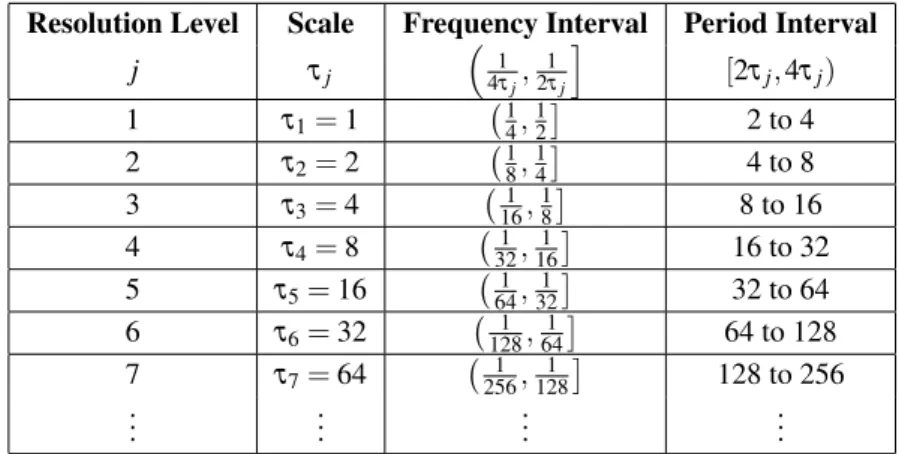
Table 1: Frequency and Period Intervals in each scaleτj=2j−1
Resolution Level Scale Frequency Interval Period Interval
j τj
1 4τj,
1 2τj
i
[2τj,4τj)
1 τ1=1 1
4, 1 2
2 to 4
2 τ2=2 1
8, 1 4
4 to 8
3 τ3=4 1
16, 1 8
8 to 16
4 τ4=8 1
32, 1 16
16 to 32
5 τ5=16 1
64, 1 32
32 to 64
6 τ6=32 1
128, 1 64
64 to 128
7 τ7=64 1
256, 1 128
128 to 256 ..
. ... ... ...
Each scaleτj related to resolution level jcorresponds to a period interval from 2τj to 4τj. The
higher the resolution level j, the smoother the scaleτj, representing the effects related to this
scale have low frequency.
The periodogram provides a good description of the predominant frequencies contained in the signal and where the significant changes are located.
3 EXPERIMENTS
we generated signals, illustrated in(b)of Figure (1), consisting of the sum of three periodic functions f,gandhof frequenciesk=12,21 and 5 (showed in(a)of Figure (1)), respectively, and a localized noisemadded to the signal. In(c)of Figure (1), the same signalsis translated from 20 units forward.
0 20 40 60 80 100 120
−6
−4
−2
0
2
4
6
Time
f g h
(a) Three periodic functions that generate the signal
0 20 40 60 80 100 120
−15
−5
0
5
10
Time
s = f + g + h + m
(b) Simulated signal s with a non-stationary behavior
0 20 40 60 80 100 120
−15
−5
0
5
10
Time
(c) Shifted signals
Figure 1: Simulated and shifted signals composed by periodic functions and a non-stationary behavior.
the scale that includes this frequency can be removed. Then, the coefficients of other scales can be reconstructed and compared to the original simulated signal(g+h+m)in the time domain.
To illustrate the shift-invariance of the NDWT also in the real data analysis, we analyzed the effects of ionospheric scintillation on GPS signals [2]. The ionospheric scintillation, caused by irregularities in the density of electrons present in the ionosphere, can weaken the signal received by the GPS receiver, causing degradation of positioning or even signal loss [3]. The main indica-tive to investigate the ionospheric scintillation impact in GPS satellite signals quality is theS4 index. In(a)of Figure (2) we show the ionospheric scintillationS4 signal in a day of weak effect of scintillation. The time series of scintillation index presents daily gaps that occur when the satellite is invisible below the horizon, and daily periodic behavior, which has a shape of ”U”, when there are data. This scintillationS4 signal was shifted some units forward (in(b)of Figure (2)) and it also was analyzed in multi-scale by DWT and NDWT.
(a) ScintillationS4 signal (b) Shifted scintillationS4 signal
Figure 2: AnalyzedS4 index time series.
4 RESULTS AND DISCUSSIONS
4.1 Simulated data
The DWT and NDWT were applied to the simulated signalsand shifted one, in order to obtain a performance comparison of both transforms in signal analysis. The Figures (3) and (4) present the DWT and NDWT periodogram of the signals, respectively.
The comparison of the obtained results in Figures (3) and (4) shows a better performance of the NDWT in the signalsanalysis. Through DWT periodogram it is not easy to extract information of the signal. The NDWT periodogram, however, spells out the periodic functions on the scales of resolution levels from 2 to 4 in addition to identifying noise in the most refined scale, which is located in the signal between the instants 40 and 50. According to Table(1), the periodic func-tionsf,gandh, respectively located on the scales of resolution levels 3,4 and 2, have frequencies in the bands from 8 to 16, 16 to 32 and 4 to 8, respectively, as expected.
Wavelet Decomposition Coefficients
Standard transform Daub cmpct on least asymm N=10Time
Resolution Le
vel
1
2
3
4
5
6
7
0 16 32 48 64
(a) DWT periodogram of signal
Wavelet Decomposition Coefficients
Standard transform Daub cmpct on least asymm N=10Time
Resolution Le
vel
1
2
3
4
5
6
7
0 16 32 48 64
(b) DWT periodogram of shifted signal
Figure 3: DWT periodogram.
Wavelet Decomposition Coefficients
Nondecimated transform Daub cmpct on least asymm N=10Time
Resolution Le
vel
1
2
3
4
5
6
7
0 32 64 96 128
(a) NDWT periodogram of signal
Wavelet Decomposition Coefficients
Nondecimated transform Daub cmpct on least asymm N=10Time
Resolution Le
vel
1
2
3
4
5
6
7
0 32 64 96 128
(b) NDWT periodogram of shifted signal
Figure 4: NDWT periodogram.
showing that the DWT is shift-variant. However, note in the Figure (4) that a translation of the input signal does not generate changes in the wavelet coefficients (in(b)) relative to the original signal (in(a)), unless than a translation. Functionality of the NDWT described herein motivates their use in the both stationary and non-stationary signal analysis.
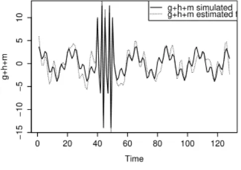
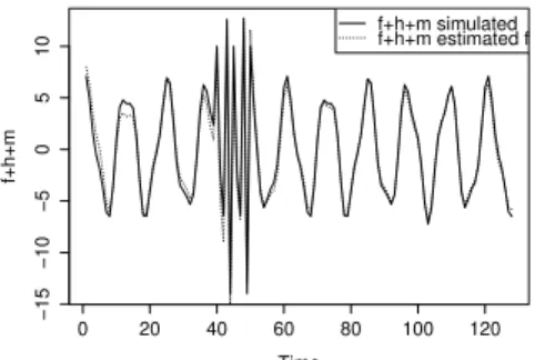
Simulations were made in order to compare the performance of the DWT and NDWT in the reconstruction analysis. Each effect concerning to the frequencies of the functions f,g,handm, which comprise the simulated signals(in(b)of Figure (1)), were singly eliminated in the multi-scale decomposition. Then the signal was reconstructed and compared to the simulated signal without such frequency. The Figures (5) and (6) present the obtained results with the DWT and NDWT, respectively. It is important to be clear, that in (a)of these Figures, for example, the estimated signal f+h+mis the reconstruction from the complete signal s= f+g+h+m
0 20 40 60 80 100 120
−15
−10
−5
0
5
10
Time
f+h+m
f+h+m simulated f+h+m estimated from s
(a) Remotion of the scale that contains the frequency of the signalg
0 20 40 60 80 100 120
−15
−10
−5
0
5
10
Time
g+h+m
g+h+m simulated g+h+m estimated from s
(b) Remotion of the scale that contains the frequency of the signalf
0 20 40 60 80 100 120
−15
−10
−5
0
5
10
Time
f+g+m
f+g+m simulated f+g+m estimated from s
(c) Remotion of the scale that contains the frequency of the signalh
0 20 40 60 80 100 120
−5
0
5
10
Time
f+g+h
f+g+h simulated f+g+h estimated from s
(d) Remotion of the scale that contains the frequency of the signalm
Figure 5: Reconstruction analysis by DWT. Simulated function and estimated function recon-structed from the complete signal s= f+g+h+m after decomposition, identification and removal of the scale that contains the frequency of interest.
The Figures (5) and (6) show the reconstruction analysis by DWT and NDWT, respectively. Note by comparing these Figures that, in both instances, the estimation from the reconstructed signal was not perfect, as expected. This fact is justified by removing an entire bandwidth of the wavelet periodogram. Even so the estimated signal closely approximates the original signal, mainly from NDWT that presents better results than DWT.
In order to compare the quality of the reconstructions obtained from the DWT and NDWT (Fig-ures (5) and (6)) we calculate the Mean Absolute Error (MAE) and Mean Squared Error (MSE) between the simulated signal and signal estimated from each wavelet decomposition. The results are presented in the Table 2.
0 20 40 60 80 100 120
−15
−10
−5
0
5
10
Time
f+h+m
f+h+m simulated f+h+m estimated from s
(a) Remotion of the scale that contains the frequency of the signalg
0 20 40 60 80 100 120
−15
−10
−5
0
5
10
Time
g+h+m
g+h+m simulated g+h+m estimated from s
(b) Remotion of the scale that contains the frequency of the signal f
0 20 40 60 80 100 120
−15
−10
−5
0
5
10
Time
f+g+m
f+g+m simulated f+g+m estimated from s
(c) Remotion of the scale that contains the frequency of the signalh
0 20 40 60 80 100 120
−5
0
5
10
Time
f+g+h
f+g+h simulated f+g+h estimated from s
(d) Remotion of the scale that contains the frequency of the signalm
Figure 6: Reconstruction analysis by NDWT. Simulated function and estimated function recon-structed from the complete signal s= f+g+h+m after decomposition, identification and removal of the scale that contents the frequency of interest.
Table 2: Mean Absolute Error (MAE) and Mean Squared Error (MSE) of signal estimated from NDWT and DWT.
Estimated signal MAE MSE MAE MSE
f+h+m 0.59 0.67 0.99 1.50
g+h+m 0.83 1.38 1.31 2.75
f+g+m 0.43 0.49 0.99 1.43
f+h+g 0.52 1.43 0.73 1.76
4.2 Real data
signal (in(b)), respectively. Through them we compared the performance of both transforms in signal analysis.
(a) DWT periodogram ofS4 signal (b) DWT periodogram of shiftedS4 signal
Figure 7: Multiscale analysis ofS4 index time series by DWT.
(a) NDWT periodogram ofS4 signal (b) NDWT periodogram of shiftedS4 signal
Figure 8: Multi-scale analysis ofS4 index time series by NDWT.
In the S4 index time series multiscale analysis, the NDWT also present better results than DWT. The comparison of the periodograms produced by DWT (Figure (7)) and NDWT (Figure (8)), shows that differently of the set of wavelet coefficients generated by DWT, the NDWT coeffi-cients of shifted signal (in(b)of figure) differ of the NDWT coefficients originalS4 signal (in (a)) only by translation of coefficients, showing that NDWT is shift-invariant also in real data analysis.
5 CONCLUSIONS
simulated and real data. Hence, we encourage the use of NDWT instead of DWT when the aims is to analyze the coefficients or investigate effects in signals or time series.
ACKNOWLEDGMENTS
Thanks to Foundation for Research Support of the State of S˜ao Paulo - FAPESP and CAPES, for the financial support.
RESUMO. Devido sua habilidade de localizac¸˜ao tempo-frequˆencia, a Transformada wavelet tem sido aplicada em v´arias ´areas de pesquisa envolvendo an´alise e processamento de dados, frequentemente substituindo a convencional Transformada de Fourier. A Transfor-mada Wavelet Discreta tem um grande potencial de aplicac¸˜ao, destacando-se como uma im-portante ferramenta na compress˜ao de sinal, processamento de imagem e sinal, suavizac¸˜ao e filtragem de ru´ıdos em dados. Ela tamb´em apresenta vantagens sobre a vers˜ao cont´ınua por causa de sua f´acil implementac¸˜ao, bom desempenho computacional e reconstruc¸˜ao per-feita do sinal ap´os invers˜ao. No entanto, a decimac¸˜ao requerida no c´alculo da Transformada Wavelet Discreta a torna variante `a translac¸˜ao e n˜ao apropriada para algumas aplicac¸˜oes, tais como an´alise de sinais ou s´eries temporais. Por outro lado, a Transformada Wavelet Discreta N˜ao Decimada ´e invariante `a translac¸˜ao, porque elimina o processo de decimac¸˜ao, e consequentemente, ´e mais apropriada para identificar comportamentos estacion´arios e n˜ao estacion´arios presentes no sinal. No entanto, a Transformada Wavelet N˜ao Decimada tem sido pouco usada na literatura. Esse artigo pretende mostrar as vantagens do uso na Transformada Wavelet N˜ao Decimada na an´alise de sinais. Os principais aspectos te´oricos e pr´aticos da an´alise multiescala de s´eries temporais a partir das wavelets n˜ao decimadas, em termos de sua formulac¸˜ao usando o mesmo algoritmo piramidal da Transformada Wavelet Decimada, s˜ao apresentados. Por fim, aplicac¸˜oes com s´eries temporais simuladas e reais comparam o desempenho das transformadas wavelet decimada e n˜ao decimada, demon-strando a superioridade da wavelet n˜ao decimada, principalmente devido `a an´alise invariante a translac¸˜ao, detecc¸˜ao de padr˜oes e uma reconstruc¸˜ao mais perfeita do sinal.
Palavras-chave: Wavelets n˜ao decimadas, invariˆancia `a translac¸˜ao, s´eries temporais, an´alise de sinais.
REFERENCES
[1] M. Ba˘sta. The MODWT analysis of the relationship between mortality and ambient temperature for Prague, Czech Republic, inActa Oeconomica Pragensia,19(2011), 20–40.
[2] G. O. N. Brassarote, E. M. Souza & J. F. G. Monico. Multiscale Analysis of GPS Time Series from Non-decimated Wavelet to Investigate the Effects of Ionospheric Scintillation, inTEMA – Tend. Mat. Apl. Comput.,16(2) (2015), 119–130.
[4] M. Gonz´alez-Aud´ıcana, X. Otazu, O. Fors & A. Seco. Comparison between Mallat’s and the ’`a trous’ discrete wavelet transform based algorithms for the fusion of multispectral and panchromatic images, inInternational Journal of Remote Sensing26(3) (2005), 595–614.
[5] A. Kumar, L. K. Joshi, A. Pal & A. Shukla. MODWT based time scale decomposition analysis of BSE and NSE indexes financial time series, inInternational Journal of Mathematical Analysis,5(27) (2011), 1343–1352.
[6] S. G. Mallat. A theory for multiresolution signal decomposition: the wavelet representation, inIEEE Trans. on Pattern Anal. and Mach.Intell.,11(1989), 674–693.
[7] G. P. Nason & B. W. Silverman. The Stationary Wavelet Transform and Some Statistical Applications, inWavelets and statistics - Springer Verlag, (1995), 281–281.
[8] D. B. Percival & A. T. Walden. Wavelet Methods for Time Series Analysis (Vol. 4), Cambridge university press, (2006).
[9] M. J. Shensa. Discrete Wavelet Transforms: The relationship of the ’`a trous’ and Mallat algorithms, in
Treizi`eme Colloque Gretsi - Juan-Les-Pins, (1991).
[10] F. Buendia, A. M. Tarquis, G. Buendia & D. Andina. Feature Extraction Via Multiresolution MODWT Analysis in a Rainfall Forecast System, inWmsci 2008: 12th World Multi-Conference on Systemics, Cybernetics and Informatics, (2008), 69–73.