where a non-random factor leads to a change in the process under control, the out-of-control process is said to be the result of a process out of control of a defective product. Random agents are also caused by the accumulation of a number of small and unavoidable deviations that in the statistical quality control process, the random factor-affected process is usually considered as the process under control. The control chart discussed in this article is a cumulative control chart that is plotted by summing the pre-self statistical samples and comparing the result with the permissible control boundary detects how the process status is used to identify cost variables. Waiting time is the unit of time and cost of identifying the cause deviation as well as the decision variables that include sample size, sampling interval, and cumulative control chart decision distance, and reference value, economic statistical design. In this paper, the econometric design of control charts is performed under the cost model of Lorenzen and Vance. This paper deals with the economic performance of the cumulative control chart and compares it with the Schuharti control chart. The economic performance of the cumulative assembly control charts is more appropriate. It is necessary to explain the distribution mechanism of the exponential distribution process failure and all calculations are programmed with R software.
Keywords: Economic statistical design. Cumulative control chart. Exponential shock model.
Resumo: Em uma ampla gama de aplicações industriais, é desejável que os processos resultem em produtos sem falhas. O processo de fabricação deve ter variabilidade limitada em torno do valor alvo para o produto. Em um processo em que um fator não aleatório leva a uma mudança no processo sob controle, diz-se que o processo fora de controle é o resultado de um processo fora de controle de um produto defeituoso. Os agentes aleatórios também são causados pelo acúmulo de vários desvios pequenos e inevitáveis que, no processo estatístico de controle de qualidade, o processo aleatório afetado por fatores é geralmente considerado como o processo sob controle. O gráfico de controle discutido neste artigo é um gráfico de controle cumulativo que é plotado pela soma das amostras pré-estatísticas e comparando o resultado com o limite de controle permitido, detecta como o status do processo é usado para identificar variáveis de custo. O tempo de espera é a unidade de tempo e custo para identificar o desvio da causa, bem como as variáveis de decisão que incluem tamanho da amostra, intervalo de amostragem e distância da decisão do gráfico de controle cumulativo e valor de referência, design estatístico econômico. Neste artigo, o design econométrico de gráficos de controle é realizado no modo custo l de Lorenzen e Vance. Este artigo trata do desempenho econômico da tabela de controle cumulativa e a compara com a tabela de controle de Schuharti. O desempenho econômico das cartas de controle cumulativas de montagem é mais apropriado. É necessário explicar o mecanismo de distribuição da falha do processo de distribuição exponencial e todos os cálculos são programados com o software R.
Master Student of Socio-Economic Statistics ,Allameh Tabataba’I University, Tehran, Iran. E-mail: [email protected] Professor, Department of statistics Faculty of Mathematical Science and Computer, Allameh Tabataba’I University. E-mail: [email protected] Bachelor Student of Computer Science at Sharif University of Technology, Tehran, Iran. E-mail: [email protected] Faezeh Najafi Mohammad Bameni Moghadam Farzaneh Najafi
ECONOMIC-STATISTICAL DESIGN OF
CUSUM CONTROL CHARTS UNDER
EXPONENTIAL SHOCK MODEL
PROJETO ECONÔMICO-ESTATÍSTICO
DE CARTAS DE CONTROLE CUSUM NO
MODELO DE CHOQUE EXPONENCIAL
1
2
3
1
2
3
Introduction
Control charts are quality improvement tools to create and maintain statistical control of manufacturing processes. Since Schwartz (1931) first introduced the control chart, various types of these tools have been developed. At the beginning of development, control charts were designed with only statistical criteria in mind, while the basic requirement for statistical control was the economic movement process. The basic idea of economic design of control charts was first put forward incompletely by Grishik and Robibe (1952) and completed by Duncan (1956) (Shrivastavaet al., 2016). The basis of statistical control charts for controlling important changes in the production process is Schwartz control charts, which were first used in Bell Telephone Laboratories. This chart is intended as the emergence of statistical process control (SPC). This was one of the first methods of quality assurance introduced in modern industry (Ridwan et al., 2017). Statistical and economic designs each have their own strengths and weaknesses. Statistical schemes generate graphs that have high power and low error rate to identify a particular change in processes; on the other hand these schemes impose more cost than economic schemes (Haq et al., 2014). On the other hand, economic plans only consider cost and ignore the statistical properties of control charts. For this reason, it was felt necessary to redesign control charts to take into account the economic aspects in addition to statistical features. In this regard, Saniga (1989) introduced the economic statistical design of control charts (Kasarapu and Vommi, 2013). One of the most powerful tools for stabilizing and improving processes is statistical process control (SPC), in which the achievements of the pre-construction steps and improvement in the specific domains specified at the time of design are performed by statistical techniques called control charts. The purpose of control charts is to address a concept called sustainability (process-controlled statistics) that performs some kind of scientific monitoring and control over the variability in process output through process behavior monitoring and while the trend or wheels are abnormal, the control charts give the audiences the necessary warning that the process is out of control and unstable. In this regard, it is worth noting that there are various ways to control and optimize process and product quality enhancement are presented, including methods statistical control, such as control charts due to the nature of random variability in the system under study are of special significance (Lai et al, 2017). The inherent variability or disruption of any production process is caused by the accumulation of a large set of small and unavoidable deviations known as «random deviations». A process that operates only in the presence of random deviations is called a statistically controlled process. In other words, random deviations are an integral part of the process. Another type of variability that is not part of random deviations is called «caused deviations» that usually originate from three sources: incorrect device configuration, user errors, and faulty raw materials (Caballero-Morales, 2013).The process that works in the presence of caused deviations is called a process out of control. Most manufacturing processes are usually in a controlled state, which allows for long-term production of acceptable products. However, at times, caused deviations can occur and cause the process to shift out of control. In this case, a large percentage of the process output will not conform to the desired requirements. Therefore, when the process shifts out of control due to deliberate deviations, a control diagram alert to detect this is the ultimate goal of drawing this chart. This will prevent the mass production of defective products. Of course, the technical responsibility of identifying caused deviation and turning the process into a controlled state that is possible by engineering methods will be the responsibility of the technical department (Seif et al., 2015). The control chart is actually the execution of a statistical hypothesis test over time. To do this, according to a sampling design, samples (random or correlated) are selected over time intervals (uniform or non-uniform). Then the desired statistic (the test statistic is calculated) and its value is specified on the chart. If this value is within the control range, the process is controlled and if it is outside the process, it is considered out of control (Shamsuzzaman et al., 2015).
Designing control charts is the main objective is to determine the optimal regulatory parameters, namely sample size, sampling interval and control limit coefficient for the process under study in four approaches: experimental design, statistical design (SD), economic design (ED) and economic- statistical- design (ESD) is performed, the empirical approach first presented by the
designer of the schwartz control chart in 1924. In his approach, sample size 4 or 5 and control limite coefficient 3 and sampling interval h = 1 (in hours) were used for high volume production processes, despite its simple experimental design and use. It is easy to operate but not economically and statistically insufficient (Faraz and Saniga, 2013). The statistical design of the sample size and the control coefficient of determination shall be such that the test capability to detect a specific changes in the quality characteristic as well as the probability of first type error being equal to a certain value. For this purpose, statistical design criteria such as type i and type ii errors are considered. The statistical design of control charts rarely takes into account the sampling interval, and usually when selecting sampling intervals, users are suggested to consider factors such as production rate, average frequency of changes that lead out of control. In many cases, the use of scientific experience and statistical criteria has led to general guidelines for the design of control charts (Mahadik, 2013). Statistical design provides high power charts and low first-rate error rates to detect specific changes in the process; this type of design fails to take into account economic aspects and imposes higher quality costs than economic design (Katebi et al., 2016). On the other hand, economic design, which aims to optimize the design parameters so as to minimize the average total cost per unit time to execute this design, considers only the cost and neglects the statistical properties of the control charts. Economic design is defined by defining quality cycles as successive time periods that begin with the system being under control and ending with a deviation due to its discovery and correction resulting in the system being restored. From the reward-renewal theorem, the average cost per quality cycle divided by the average time of that cycle results in the average cost per unit time for that cycle, which will be the objective function of the minimization problem (Heydari et al.,2016). Woodall (1986), as a critic of the economic designs of the control charts, showed that these schemes significantly increased the probability of the first type of control chart error than the statistical design. This increase in the likelihood of the first type of error can lead to increased false alarms and correction over process startup. Unnecessary process adjustments often increase variability and change in quality attributes, and over time cause managers and industry owners to lose confidence in control charts (Rafiey et al., 2016). In designing a variable control chart we have a quality attribute designed to monitor the process behavior of this quality attribute. On the other hand, today, technological advancements have complicated the production processes of a product (product or service), and the simultaneous control of two or more interrelated and independent quality characteristics in the process seems necessary. To control for these quality characteristics, considering a set of one-variable control charts for each variable can lead to very misleading results. The establishment of an efficient and reliable multi-control diagram will reduce the costs of internal and external quality failure, despite an increase in preventive costs (Mahadik, 2013).
The economic design of control charts is based solely on cost minimization and does not interfere with statistical criteria. In order to overcome this problem, Saniga (1989) proposed a statistical-economic design. This design eliminates the disadvantages of economic design by taking into account both statistical and economic aspects. Economic- statistical design charts need a distribution for the process failure mechanism to determine the optimal design parameters (Albloushi et al., 2015).
Aghabeig and Moghadam (2014) investigated the economical design of the X-ray development under a generalized view distribution failure mechanism with uniform sampling intervals. In this paper, the economic statistical design of X control charts under the generalized view distribution fracture mechanism with uneven sampling interval is discussed. The structure of this paper is that we first introduce economic-statistical design of cusum control charts in section 1 and then in section 2 we prepare cost models and also elaborating Shewhart and CUSUM chart in section 3 and 4 respectively. We compare the numerical results of statistical-economic design and economic design in section 5. And finally in section 6, the conclusion is discussed.
Cost models
We consider a production process that operates indefinitely. There is only one quality attribute that needs to be monitored, and that quality attribute is a normal random variable with a target value of and the variance is . Note that the variance is in fact known and unknown, but we assume that it can be accurately estimated from past data. Also note that the assumption of normality, which is somehow found in most related texts and sources, is practically harmless when sample sizes are not too small because sample averages are, however, approximately approximated by the central limit theorem have normal distribution. However, if the distribution has obvious and significant deviations from the normal distribution and the sample sizes are small or unit, then the economic performance analysis of the CUSUM and Schuharty charts should be modified accordingly and beyond this scope. Process from statistical control mode (under control) it starts and is subject to two free deviations (deviation 1 and deviation 2) that average the process from transfer to or . The occurrence of these deviations causes the process to shift out of control. It is assumed that the times of cause deviations 1 and 2 are independent exponential random variables with averages of and , respectively. Thus, the expected time until any deviation occurs is for which . The probability that a cause deviation will occur at a time interval, provided that the process is controlled at the beginning of this interval, is a function of and is:
(1)
The probability that the deviation with reseaon -th (j = 1 or = 2) before the other deviation in the time interval occurs is: (2) It is assumed that after the deviation with reseaon -th, the average process remains at until it reaches us again. At each sampling time, a sample of size is taken, the mean of the sample calculated and a warning may be issued depending on its value and chart statistics. If no warnings have been issued for the chart, no action is taken and subsequent sampling begins just after time unit. If an alert is issued, investigations begin and if a deviation is detected the process returns to control state. It should be noted that the process can be stopped or continued during the search and repair. It is assumed that the time for sampling and study after a false alarm is less than . As a result, the sampling process stops during study and correction because sampling is useless when the process is found to operate out of control. After detecting and eliminating a real deviation, the operation process resumes its operation from control state, and then the next sample is taken after time unit. The cost of sampling and inspection is c per unit and the fixed cost for each sample is b. The cost of a false alert is L., and the cost of restoring the process after a alert is . The other expected costs per unit time of operation are M when the process operates out of control. Due to the weaknesses of statistical designs and economic designs, another method was proposed in the design of control charts that take into account the economic aspects in addition to statistical properties (Sultana et al., 2016). In this regard, Saniga (1989) eliminated the weakness of economic design by placing statistical constraints (depending on the design requirement) and termed it economic statistical design. This design eliminates the disadvantages of statistical schemes and economic schemes while simultaneously taking into account statistical and economic aspects and is in fact a good alternative to them(). Due to statistical constraints, economic statistical plans impose a higher cost than economic plans on the system. But due to the low rate of false alarms and reduced process variability that leads to improved quality, it is in line with statistical
quality control objectives while controlling product quality costs at a desirable level of error and high power(Montgomery, 2018). In this section, we also use Markov chains to provide a model for economically optimizing Shewhart and CUSUM charts. Specifically, we use a two-dimensional time-discrete Markov chain describing: (1) the actual state of the process (a process under statistical control or under the influence of a cause deviation); and (2) a decision that samples are taken each time. We begin by describing this approach by elaborating the Markov model for the Schwarz chart.
Shewhart chart
For the Schwartz chart with control limits , the probability of the first type error is and the probability of the second type error is
. Let represent the actual state of the process at the sampling time t where represents the state under control
for the state out of the control and for the state out of control
. If, at the time of sampling t th, the absolute value of the mean standardized sample is exceeds the control limit
, an alert issued based on the process to be out of control, and then initiates the necessary steps to the process. The decision is represented by . Otherwise, when it is
, then no action is taken . Random time-discrete model for the process and its supervision scheme, based on the combination of the actual state of the process is and the value is at t. The pair ( , ) represents the state of a two-dimensional time-discrete Markov chain (DTMC) with specific features that each step may take when measuring in real time units have different periods of time. There are six possible modes and the probability matrix of the transfer is as follows:
Figure 1: Time between two consecutive sampling associated with the exit of each of the six Markov chains 3
The steady-state probabilities ( , ), denoted by the symbol , can be obtained by solving the system of linear steady state equations and can be used to estimate the expected long-term cost in time unit as the ratio of the average cost of a transition step over its average duration: if is the expected cost and the duration of a transition from state to a different or identical state at the next sampling, then the expected long-term cost at each unit time is: (3) More specifically, the expected costs of between two consecutive sampling periods associated with existing each of the six possible Markov chains are: If the chart does not issue any alarts the time to next sampling is only equal to . But if an alert is issued, the length of time is increased by the number of study times and correction, unless the alert is false and the process continues during the study ; then T is part of , assuming that its value does not exceed
. Note that the value of appears in all high-cost terms, , because the sampling cost is constant regardless of the state of the process
. Cost of a false alert, , only appears in because state (0,1) is the only state associated with a false alert. Similarly, the cost of process correction after a true alert, , only appears in , . The other expected costs resulting from the performance of the process under the influence of a cause deviation during the interval are somewhat less obvious, as this quantity depends on the expected time during which the process operates out of control. This charge is equal to the value of for distances starting from and from DTMIC, since these states represent a second type error of the chart and thus the operation is out of process control for the entire interval until the next sample. The cost of
is borne by the system during the operational time before eliminating a cause deviation when or
. Finally, is the expected cost of being out of control of the system at intervals, provided that the system is controlled at the beginning of this interval, i.e., when DTMIC is in state or and this cost is also subject to elimination after eliminating an cause deviation when (1 = Y = 1, at) or ( Y=2, 4=1); in particular, if π represents the conditional expected time on a cause deviation from a given interval, provided that such an event occurs in that interval, then the process affected by it for an expected time will work.
As a result, the unconditional expected time for performance out of control at a time interval in which the process begins its activity in a controlled state is equal to . Duncan’s studies (1956) have shown that
and since we have . Therefore, the expected cost corresponding to state out of control is equal to . By grouping similar cost terms together, Equation (3) can be simplified as follows: (4)
In the special case or
, the steady state probabilities are:
(5) The above phrase is almost identical to the corresponding one in the studies of Lorenzen and Vance (1). There is only one small difference in the cost of sampling, which is due to different assumptions in their model, that way, the sampling never stops as long as the process works.
CUSUM chart
To monitor the process average using the CUSUM chart, the usual method is to use two separate CUSUM statistics, for example, to detect upstream transitions and to detect downstream transitions.,
Where is mean of the standardized sample and is the reference value of the CUSUM chart. An alert is issued when both statistics exceed the H control limit. An alternative method, proposed by Crosier (1986), uses only one statistic that can have positive or negative values: , An alarm time is issued when or is set. The Markov chain which describes the evolution of the process at the time of observation by the CUSUM type chart is equivalent to {...0٫٫٫٫٫ = ) , t )} where is the actual state of the process and is the value of the CUSUM statistic in the sample t. For practical purposes, the value of
to , which follows the Brook and Evans (1972) approach. Using the above discontinuity, the Markov chain has a
possible state ( and ) with the probability of transferring it as follows:
(6) Consequently, the probability matrix of the transfer would be as follows:
The above matrix elements are divided into nine parts, which include the probability of moving from to C for each of the nine possible combinations of and
. The exact expressions for the probabilities of are given below. Similarly to the Schwartz charts, the steady-state probabilities of for
(i = 0, 1, 2, j = m….m) are used to estimate the expected cost per unit time used, it can be written as follows:
(7)
The cost function, ECT2, is the exact form of ECT1 for the CUSUM charts, and the explanation
of all its quantities is similar to the ECT1 terms. Note that this Markov model does not require explicit calculation and ARL.
Numerical comparison
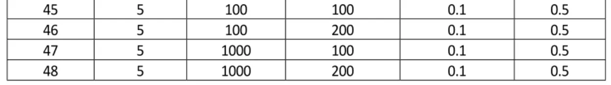
We perform numerical analysis to investigate the potential cost savings of choosing a CUSUM chart instead of choosing a Schwartz chart to monitor a process. The numerical investigation covers three cases covering a wide range of cost parametersand process parameters ( ) as shown in Table 1. In all 48 cases, certain parameters were kept constant: repair cost L1=200 and negligible time to seek a cause deviation and correction process: 0 = T2 = T. = T1. Although the models are adaptable enough to accommodate non-negligible search and modification times, our numerical investigation has shown that the effect of these times on process design parameters and costs is minimal and, therefore, due to cost savings and simplicity, we set their values to zero. We also assume that the process stops after the alert is declared for review ( ). In addition, when the system is repaired and restored after a proper alert the process is stopped ( ). Finally, we set the relation in all cases.
For each specific set of parameters, we first determine the economic design of the Schwartz chart with respect to Equation (7) and then compare them with the optimal parameters and cost of the CUSUM chart obtained from the equation. To expedite the optimization procedure, we allow and to be integers of 0.1, and by setting , we use a similar discrete step for the control limit H in the CUSUM chart with an initial value of 0.05 (m = 1). Note that the number of states used to discrete Markov chains of CUSUM chart, with , depends on the actual value of H in each case. Table 2 shows the optimal parameters and costs of the Schwartz and CUSUM charts for the 48 items in Table 1. The percentages of profits from using the CUSUM chart instead of the Schwartz chart are shown in the last column of Table 2. Table 2 shows that the sampling interval and sample size of the CUSUM scheme are not significantly different from those corresponding to the Schwartz scheme. In particular, in many cases, both the optimal parameters and for the CUSUM chart are partially smaller than and corresponding to the Schwartz chart. The improvement in the cost of the CUSUM chart was less than 0.7% over all 48 cases we reviewed.
As a result, it is clear that from the economic point of view the CUSUM chart is not significantly superior to the standard chart, even when the rate of change is small. Note that Ho (1994), although their numerical results were very similar to ours, concluded that the CUSUAL chart works much better than the standard chart. More importantly, our results are also inconsistent with the results obtained by Keats and Simpson (1994), who found that the CUSUM chart performs significantly better than the Schwartz chart. Our guess is that this inconsistency may be due to the inaccuracy of the calculations and the use of in the model to economically optimize the CUSUM scheme. The results in Table 2 are surprising given the widespread understanding that CUSUM chart are far more effective than Schwartz chart, at least in detecting small to medium displacements. Given the above observations and concerns, we first validate the results of Table 2 by simulation and then extend the numerical investigation to improve our findings. Finally, it should be emphasized that there are many practical applications where sample sizes are not necessarily uniform, but they are limited to relatively small amounts for logical grouping or other reasons. Limiting the sample size, such as , can cause the CUSUM chart to perform significantly better than its corresponding Schwartz chart, unless the sample size without the optimal limit is greater than five. The difference in the economic performance of these two charts, if there is a limit on the sample size, is somewhere between the differences observed in the case of n infinite and n = 1. For example, consider item 1 of Table 1 with c = 1. If there is no limit on sample size, we can see from Table 2 that both sample sizes are relatively large and have approximately identical average costs: ECT1 = 11.76 with n = 24 Schwartz chart and ECT2= 11.72 with n = 23 for the CUSUM
chart.
If the sample size is restricted by for logical grouping, then the average cost of the two constrained chart (n = 5) is equal to ECT1 = 12.14 and ECT2 = 12.39 (a difference of 12.3%). If
and ECT2 = 12.57 and the CUSUM economic advantage increased by 7.14%. Table 1: Set of 48 parameters for numerical example Case 1 0 100 100 0.01 0.5 2 0 100 200 0.01 0.5 3 0 1000 100 0.01 0.5 4 0 1000 200 0.01 0.5 5 5 100 100 0.01 0.5 6 5 100 200 0.01 0.5 7 5 1000 100 0.01 0.5 8 5 1000 200 0.01 0.5 9 0 100 100 0.1 0.5 10 0 100 200 0.1 0.5 11 0 1000 100 0.1 0.5 12 0 1000 200 0.1 0.5 13 5 100 100 0.1 0.5 14 5 100 200 0.1 0.5 15 5 1000 100 0.1 0.5 16 5 1000 200 0.1 0.5 17 0 100 100 0.01 0.5 18 0 100 200 0.01 0.5 19 0 1000 100 0.01 0.5 20 0 1000 200 0.01 0.5 21 5 100 100 0.01 0.5 22 5 100 200 0.01 0.5 23 5 1000 100 0.01 0.5 24 5 1000 200 0.01 0.5 25 0 100 100 0.1 0.5 26 0 100 200 0.1 0.5 27 0 1000 100 0.1 0.5 28 0 1000 200 0.1 0.5 29 5 100 100 0.1 0.5 30 5 100 200 0.1 0.5 31 5 1000 100 0.1 0.5 32 5 1000 200 0.1 0.5 33 0 100 100 0.01 0.5 34 0 100 200 0.01 0.5 35 0 1000 100 0.01 0.5 36 0 1000 200 0.01 0.5 37 5 100 100 0.01 0.5 38 5 100 200 0.01 0.5 39 5 1000 100 0.01 0.5 40 5 1000 200 0.01 0.5 41 0 100 100 0.1 0.5 42 0 100 200 0.1 0.5 43 0 1000 100 0.1 0.5 44 0 1000 200 0.1 0.5
45 5 100 100 0.1 0.5
46 5 100 200 0.1 0.5
47 5 1000 100 0.1 0.5
48 5 1000 200 0.1 0.5
Table 2: Comparison of Schwartz chart with CUSUM charts (c = 1) Schwartz optimization Optimization of CUSUM
Case Percentage of cost improvement (%) 1 7.2 24 1.6 11.76 6.9 23 1.1 0.6 11.72 5.65 0.4 2 8.3 32 1.9 12.64 7.8 30 1.3 0.7 12.59 16.82 0.4 3 2.2 24 1.6 33.92 2.1 23 1.1 0.6 33.77 - 0.4 4 2.5 34 2.0 36.81 2.4 31 1.3 0.7 36.64 - 0.5 5 8.3 27 1.6 12.41 8.0 26 1.1 0.6 12.39 - 0.2 6 9.1 34 1.9 13.22 9.0 34 1.4 0.6 13.19 22.85 0.2 7 2.6 28 1.6 36.01 2.5 27 1.2 0.5 35.94 7.00 0.2 8 2.8 35 1.9 38.69 2.7 34 1.4 0.6 38.58 - 0.3 9 2.8 21 1.5 45.46 2.6 20 0.9 0.7 45.32 - 0.3 10 3.2 28 1.8 47.70 3.0 26 1.1 0.8 47.53 9.82 0.4 11 0.7 23 1.6 1117.66 0.7 23 1.1 0.6 117.18 - 0.4 12 0.8 31 1.9 126.46 0.8 31 1.3 0.7 125.90 - 0.4 13 3.3 23 1.4 47.13 3.2 22 0.9 0.6 47.05 - 0.2 14 3.6 31 1.8 49.17 3.5 30 1.2 0.7 49.08 - 0.2 15 0.8 26 1.6 124.09 0.8 26 1.1 0.6 123.86 - 0.2 16 0.9 34 1.9 132.18 0.9 34 1.4 0.6 131.86 - 0.2 17 4.4 10 2.2 7.82 4.4 10 1.5 0.8 7.79 - 0.4 18 4.7 12 2.5 8.20 4. 7 12 1.7 0.9 8.16 - 0.5 19 1.4 10 2.2 20.82 1.3 10 1.6 0.7 20.72 - 0.5 20 1.6 13 2.5 22.03 1.4 12 1.7 0.9 21.90 - 0.6 21 5.9 12 2.2 8.78 5.8 12 1.7 0.6 8.77 - 0.1 22 6.3 14 2.4 9.09 6.2 14 1.9 0.6 9.08 - 0.2 23 1.8 12 2.2 23.91 1.8 12 1.7 0.6 23.89 - 0.1 24 1.9 14 2.5 24.93 1.9 14 1.9 0.6 24.88 - 0.2 25 1.7 10 2.2 35.90 1.5 9 1.4 0.9 35.80 2.37 0.3 26 1.9 12 2.4 36.90 1.7 11 1.6 0.9 36.78 - 0.3 27 0.5 11 2.2 78.39 0.4 9 1.5 0.8 77.95 2.35 0.6 28 0.5 13 2.5 81.97 0.5 12 1.7 0.8 81.66 - 0.4 29 2.2 11 2.1 38.48 2.2 11 1.6 0.6 38.45 - 0.1 30 2.3 13 2.4 39.30 2.3 13 1.8 0.6 39.27 - 0.1 31 0.6 12 2.2 87.81 0.6 12 1.7 0.5 87.75 - 0.1 32 0.6 14 2.5 90.96 0.6 13 1.8 0.7 90.82 - 0.2 33 2.7 4 2.8 5.31 2.2 3 1.7 1.1 5.29 - 0.4 34 2.8 4 2.9 5.46 2.7 4 2.0 1.0 5.44 - 0.5 35 0.9 4 2.7 12.46 0.7 3 1.7 1.1 12.57 - 0.6 36 0.9 4 2.9 13.14 0.8 4 2.0 1.1 13.5 - 0.7 37 4.6 5 2.7 6.71 4.5 5 2.2 0.6 6.71 - 0.0 38 4.5 5 2.9 6.81 4.6 5 2.3 0.6 6.81 - 0.0 39 1.4 5 2.7 17.13 1.4 5 2.2 0.6 17.12 - 0.1 40 1.4 5 2.9 17.47 1.4 5 2.3 0.6 17.46 0.98 0.0 41 1.0 4 2.8 29.26 0.8 3 1.7 1.1 29.16 - 0.3
42 1.0 4 2.9 29.66 1.0 4 2.0 1.0 29.59 - 0.2 43 0.3 4 2.7 53.17 0.2 3 1.7 1.2 53.02 - 0.3 44 0.3 4 2.9 54.75 0.3 4 2.0 1.0 54.52 - 0.4 45 0.3 5 2.7 33.11 1.6 4 2.0 0.6 33.11 - 0.0 46 1.7 5 2.9 33.38 1.7 5 2.2 0.7 33.36 - 0.0 47 0.5 5 2.7 67.26 0.5 5 2.2 0.5 67.26 - 0.0 48 0.5 5 2.8 68.34 0.5 5 2.2 0.7 68.29 - 0.1 Following the various constraints on these values, we present the results of the statistical-economic design of the CUSUM diagram. Table 3: Results of statistical-economic design of the CUSUM chart (c = 1) Optimization of CUSUM Case Percentage of cost improvement (%) 1 4.28 13 1.05 0.6 13.27 2.84 13 2 3.08 15 1.59 0.7 15.36 7.18 22 6 3.16 15 1.52 0.6 17.34 5.59 31 7 3.40 15 0.62 0.5 36.8 1.86 2.3 10 5.14 20 0.76 0.8 48.90 3.90 2.8 25 4.47 6 086 0.9 40.51 1.42 13 27 0.90 8 1e 0.8 94.08 1.70 20 40 1.34 1 1.5 0.6 32.73 0.57 87 Note that the above equation or other different methods can be used to calculate . In this paper, the equation with and is used.
Conclusion
We propose a simple and accurate Markov chain model for economically optimizing the Schwartz charts and the CUSUM to monitor the average quality characteristic with a normal distribution. Our numerical investigation led to the following results. CUSUM charts are economically superior to Schwartz charts only when process monitoring is based on individual measurements (sample size = n). If there is no limit on the size of each sample, the economic performance of the optimal CUSUM charts almost equals that of the optimal Schwartz charts, even when the predicted change is small. Between the two, where the sample size is limited to small quantities for reasons such as the need for logical grouping and also small-scale variations, the CUSUM chart can perform significantly better than the Schwartz chart. From a pure economic point of view, and in the absence of sample size constraints, the usual choice of n = 4 or n = 5 for both family Schwartz charts and for CUSUM charts is always less important than larger ones in detecting small deviations. Sample size n٫ > can only be economically feasible if the projected change in the mean of the process involves medium to large values and the cost of sampling is very low. 3. When the sample size is strictly limited to n = 1 or when the sampling cost is very high and the rate of change is small, it is usually not optimal to monitor the process through sampling but rather to control it using a preventive maintenance policy can be very desirable. As a result, this option should always be considered as an alternative to the usual SPC method.
References
Aghabeig D. and Moghadam M. (2014). “Economic design of -control charts under generalized exponential shock models with uniform sampling intervals,” European Online Journal of Natural and Social Sciences, vol. 2, no. 3, 2014.
Albloushi T., Suwaidi A., Zarouni N., Abdelrahman A., and Shamsuzzaman M. (2015). “Design of and R control charts for monitoring quality of care for hypertension,” in Proceedings of the 5th International Conference on Industrial Engineering and Operations Management (IEOM ‘15), pp. 1–5, Dubai, United Arab Emirates, March 2015.
Caballero-Morales S. O. (2013). Economic statistical design of integrated X-bar- S control chart with preventive maintenance and general failure distribution,” PLoS ONE, vol. 8, no. 3, Article ID e59039, 2013.
Crosier, R.B. (1986). A new two-sided cumulative sum quality control scheme. Technometrics, 28, 187–194.
Duncan, A. J. (1956). The economic design of X charts used to maintain current control of a process , Journal of the American Statistical Association, 51, 228–242.
Faraz A. and Saniga E. (2013). “Multi objective Genetic Algorithm Approach to the Economic Statistical Design of Control Charts with an Application to X and S2 Charts,” Quality and Reliability Engineering International, vol. 29, no. 3, pp. 407–415, 2013.
Haq A., Brown J. & Moltchanova E. (2014). “New exponentially weighted moving average control charts for monitoring process mean and process dispersion”, Quality and Reliability Engineering International, Vol. 31(8), pp. 1587-1610, 2014.
Heydari A.A., Bameni Moghadam M. and Eskandari F (2016). An Extension of Banerjee and Rahim Model in Economic and Economic-Statistical Designs for Multivariate Quality Characteristics under Burr XII Distribution. Communications in Statistics -Theory and Methods,D OI:10.1080/03610926.2016.1140782.
Ho, C. (1994). Economic design of control charts: a literature review for 1981-1991, Journal of Quality Technology, 26, 39–53.
Kasarapu V. and Vommi B. (2013). “Economic design of chart using differential evolution,” International Journal of Emerging Technology and Advanced Engineering, vol. 3, no. 4, pp. 541–548, 2013.
Katebi, M., Seif A. and Faraz A. (2016). Economic and Economic-Statistical designs of the T2 control charts with SVSSI sampling scheme. Communications in Statistics -Theory and Methods. 46 (20):10149-10165, DOI:10.1080/03610926.2016.1231823.
Keats, J.B. and Simpson, J.R. (1994) Comparison of the X and the CUSUM control charts in an economic model. Economic Quality Control, 9, 203–220.
Lai M., Chen C. and Hariguna T. (2017). A bivariate optimal replacement policy with cumulative repair cost limit for a two-unitsystem under shock damage interaction,Brazilian Journal of Probability and Statistics, 2, 353-372.
Lorenzen T. J. and Vance L. C. (1986). The Economic Design of Control Charts: A Unified Approach, Technometrics, 28(1), 3-10. Roberts, S.W, (1959). Control chart tests based on geometric moving averages, Technometrics, 42(1), 97–102.
Mahadik S. B. (2013). Variable sample size and sampling interval charts with runs rules for switching between sample sizes and sampling interval lengths, Quality and Reliability Engineering International, 29(1):63-76.
Mahadik S. B. (2013). Charts with Variable Sample Size, Sampling Interval, and Warning Limits, Quality Reliability Engineering International, 29(4):535-544.
Rafiey S.R., Ghaderi M.M., and Bameni Moghadam M. (2016). A Generalized Versionof Banerjee and Rahim Model In Economicand Economic Statistical Designs of Multivariate Control Charts under Generalized Exponential Shock Model, Communications in Statistics -Theory and Methods. DOI:10.1080/03610926.2016.1171354.
Ridwan A. Sanusi, Mu’azu Ramat Abujiya , Muhammad Riaz , Nasir Abbas (2017). Combined Shewhart CUSUM charts using auxiliary variable. Journal of Computers and Industrial Engineering archive, 105(C), 329-337.
Saniga, E.M. (1977). Joint economically optimal design of X and R control charts. Management Science, 24, 420–431.
Seif, A. Faraz, and E. Saniga. (2015). Economic statistical design of the VP X control charts for monitoring a process under non-normality,” International Journal of Production Research, vol. 53, no. 14, pp. 4218–4230, 2015.
Shamsuzzaman M., Alsyouf I., and Ali A. (2015). “Optimization design of Xfi & EWMA control chart for minimizing mean number of defective units per out-of-control case,” in Proceedings of the IEEE International Conference on Industrial Engineering and Engineering Management, IEEM 2015, pp. 391–395, Singapore.
Shrivastava D., Kulkarni MS.,Vrat P. (2016). “Integrated design of preventive maintenance and quality control policy parameters with CUMSUM chart”, Int J Adv Manuf Technolgy, Vol. 82(9),pp. 2101-2112, 2016.
Sultana I., Ahmed I., Azeem A. & Sarkar N. (2016). “Economic Design of Exponentially Weighted Moving Average Chart with Variable Sampling Interval at Fixed Times Scheme incorporating Taguchi Loss Function”, international Journal of Industrial and Systems Engineering, 2016.
Recebido em 20 de dezembro de 2019. Aceito em 21 de fevereiro de 2020.