Artigo
*e-mail: [email protected]
QUANTITATIVE STRUCTURE–RETENTION RELATIONSHIPS ANALYSIS OF RETENTION INDEX OF ESSENTIAL OILS
Hadi Noorizadeh*, Abbas Farmany and Mehrab Noorizadeh
Department of Chemistry, Faculty of Science, Islamic Azad University, Ilam Branch, Ilam, Iran
Recebido em 7/3/10; aceito em 12/8/10; publicado na web em 30/11/10
Genetic algorithm and multiple linear regression (GA-MLR), partial least square (GA-PLS), kernel PLS (GA-KPLS) and Levenberg-Marquardt artiicial neural network (L-M ANN) techniques were used to investigate the correlation between retention index (RI) and descriptors for 116 diverse compounds in essential oils of six Stachys species. The correlation coeficient LGO-CV (Q2) between experimental and predicted RI for test set by GA-MLR, GA-PLS, GA-KPLS and L-M ANN was 0.886, 0.912, 0.937 and 0.964, respectively. This is the irst research on the QSRR of the essential oil compounds against the RI using the GA-KPLS and L-M ANN.
Keywords: essential oils; genetic algorithm-kernel partial least squares; Levenberg-Marquardt artiicial neural network.
INTRODUCTION
An essential oil is a volatile mixture of organic compounds derived from odorous plant material by physical means.1 The
com-position of essential oil has been extensively investigated because of its commercial interest in the fragrance industry (soaps, colognes, perfumes, skin lotion and other cosmetics), in aromatherapy (re-laxant), in pharmaceutical preparations for its therapeutic effects as a sedative, spasmolytic, antioxidant, antiviral and antibacterial agent.2,3 Recently it has also been employed in food manufacturing
as natural lavouring for beverages, ice cream, candy, baked goods and chewing gum. Stachys L. (Lamiaceae, Lamioideae) is among the largest genera of Lamiaceae. Stachys consists of annual and perennial herbs and subshrubs showing extensive variation in mor-phological and cytological characters.4Stachys L. is a large genus
comprising over 300 worldwide species and is widely spread throu-ghout Northern Europe and the Mediterranean.5 The constituents
of essential oil of these spices includes: oxygenated monoterpenes, monoterpene hydrocarbons, oxygenated sesquiterpenes, sesquiter-pene hydrocarbons, carbonylic compounds, phenols, fatty acids and esters. These entire compounds have been identiied by gas chromatography (GC) and gas chromatography-mass spectrometry (GC–MS). GC and GC–MS are the main methods for identiication of these volatile plant oils. To increase the reliability of the MS identiication, comprehensive two-dimensional GC–MS can be used. This technique is based on two consecutive GC separations, typically according to boiling point and polarity.6 The compounds
are identiied by comparison of retention index with those repor-ted in the literature and by comparison of their mass spectra with libraries or with the published mass spectra data.7
Chromatographic retention for capillary column gas chromatogra-phy is the calculated quantity, which represents the interaction between stationary liquid phase and gas-phase solute molecule. This interaction can be related to the functional group, electronic and geometrical properties of the molecule.8,9
Mathematical modeling of these interactions helps chemists to ind a model that can be used to obtain a deep understanding
about the mechanism of interaction and to predict the retention index (RI) of new or even unsynthesized compounds.10 Building
retention prediction models may initiate such theoretical approach, and several possibilities for retention prediction in GC. Among all methods, quantitative structure-retention relationships (QSRR) are most popular. In QSRR, the retention of given chromatographic system was modeled as a function of solute (molecular) des-criptors. A number of reports, deals with QSRR retention index calculation of several compounds have been published in the literature.11-13 The QSRR/QSAR models apply to multiple linear
regression (MLR) and partial least squares (PLS) methods often combined with genetic algorithms (GA) for feature selection.14,15
Because of the complexity of relationships between the proper-ty of molecules and structures, nonlinear models are also used to model the structure–property relationships. Levenberg -Marquardt artiicial neural network (L-M ANN) is nonparametric nonlinear modeling technique that has attracted increasing interest. In the recent years, nonlinear kernel-based algorithms as kernel partial least squares (KPLS) have been proposed.16,17 The basic idea of
KPLS is irst to map each point in an original data space into a feature space via nonlinear mapping and then to develop a linear PLS model in the mapped space. According to Cover’s theorem, nonlinear data structure in the original space is most likely to be linear after high-dimensional nonlinear mapping.18 Therefore,
EXPERIMENTAL Data set
Retention index of essential oils of six Stachys species, S. cretica L. ssp. vacillans Rech. il., S. germanica L., S. hydrophila Boiss., S. nivea Labill., S. palustris L. and S. spinosa L., obtained by hydrodistillation, was studied by GC and GC–MS, which contains 116 compounds19
(Table 1). This set was measured at the same condition with the Inno-wax column (60 m x 0.25 mm i.d.; 0.33 µm ilm thickness) for GC measurement. GC–MS analysis was also performed on an Agilent 6850 series II apparatus, itted with a fused silica HP-1 capillary column (30 m x 0.25 mm i.d.; 0.33 µ m ilm thickness). The retention index of these compounds was decreased in the range of 3710 and 1075 for both Octadecanoic acid and α-Pinene, respectively.
In order to evaluate the generated models, we used leave-group-out cross validation (LGO-CV). Cross validation consists of the follo-wing: removing one (leave-one-out) or groups (leave-group-out) of compounds in a systematic or random way; generating a model from the remaining compounds, and predicting the removed compounds.
Descriptor calculation
All structures were drawn with the HyperChem software (version 6). Optimization of molecular structures was carried out by semi-empirical AM1 method using the Fletcher- Reeves algorithm until the root mean square gradient of 0.01 was obtained. Since the calculated values of the electronic features of molecules will be inluenced by the related conformation. Some electronic descriptors such as dipole moment, polarizability and orbital energies of LUMO and HOMO were calculated by using the HyperChem software. Also optimized structures were used to calculate 1497 descriptors by DRAGON software version 3.20
Software and programs
A Pentium IV personal computer (CPU at 3.06 GHz) with windows XP operational system was used. Geometry Optimization was perfor-med by HyperChem (version 7.0 Hypercube, Inc.), Dragon software was used to calculate of descriptors. MLR analysis was performed by the SPSS Software (version 13, SPSS, Inc.) by using enter method for model building. Minitab software (version 14, Minitab) was used for the simple PLS analysis. Cross validation, GA-MLR, GA-PLS, GA-KPLS, L-M ANN and other calculation were performed in the MATLAB (Version 7, Mathworks, Inc.) environment.
THEORY Genetic algorithm
Genetic algorithm has been proposed by J. Holland in the early 1970s but it was possible to apply them with reasonable computing times only in the 1990s, when computers became much faster. GA is a stochastic method to solve the optimization problems, deined by itness criteria applying to the evolution hypothesis of Darwin and different genetic functions, i.e., crossover and mutation.21 In GA, each individual
of the population, deined by a chromosome of binary values as the coding technique, represented a subset of descriptors. The number of genes at each chromosome was equal to the number of descriptors. The population of the irst generation was selected randomly. A gene was given the value of one, if its corresponding descriptor was included in the subset; otherwise, it was given the value of zero.22 The GA performs
its optimization by variation and selection via the evaluation of the
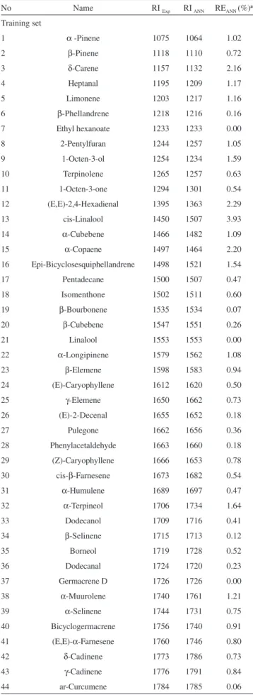
Table 1. The data set and the corresponding observed and predicted RI values by L-M ANN for the training and test sets
No Name RI Exp RI ANN REANN (%)a
Training set
1 α -Pinene 1075 1064 1.02
2 β-Pinene 1118 1110 0.72
3 δ-Carene 1157 1132 2.16
4 Heptanal 1195 1209 1.17
5 Limonene 1203 1217 1.16
6 β-Phellandrene 1218 1216 0.16
7 Ethyl hexanoate 1233 1233 0.00
8 2-Pentylfuran 1244 1257 1.05
9 1-Octen-3-ol 1254 1234 1.59
10 Terpinolene 1265 1257 0.63
11 1-Octen-3-one 1294 1301 0.54
12 (E,E)-2,4-Hexadienal 1395 1363 2.29
13 cis-Linalool 1450 1507 3.93
14 α-Cubebene 1466 1482 1.09
15 α-Copaene 1497 1464 2.20
16 Epi-Bicyclosesquiphellandrene 1498 1521 1.54
17 Pentadecane 1500 1507 0.47
18 Isomenthone 1502 1511 0.60
19 β-Bourbonene 1535 1534 0.07
20 β-Cubebene 1547 1551 0.26
21 Linalool 1553 1553 0.00
22 α-Longipinene 1579 1562 1.08
23 β-Elemene 1598 1583 0.94
24 (E)-Caryophyllene 1612 1620 0.50
25 γ-Elemene 1650 1662 0.73
26 (E)-2-Decenal 1655 1652 0.18
27 Pulegone 1662 1656 0.36
28 Phenylacetaldehyde 1663 1660 0.18
29 (Z)-Caryophyllene 1666 1653 0.78
30 cis-β-Farnesene 1673 1682 0.54
31 α-Humulene 1689 1697 0.47
32 α-Terpineol 1706 1734 1.64
33 Dodecanol 1709 1716 0.41
34 β-Selinene 1715 1713 0.12
35 Borneol 1719 1728 0.52
36 Dodecanal 1724 1720 0.23
37 Germacrene D 1726 1726 0.00
38 α-Muurolene 1740 1761 1.21
39 α-Selinene 1744 1731 0.75
40 Bicyclogermacrene 1756 1740 0.91
41 (E,E)-α-Farnesene 1760 1746 0.80
42 δ-Cadinene 1773 1786 0.73
43 γ-Cadinene 1776 1791 0.84
44 ar-Curcumene 1784 1785 0.06
itness functionη. Fitness function was used to evaluate alternative descriptor subsets that were inally ordered according to the predictive performance of related model by cross validation. The itness function was proposed by Depczynski et al..23 The root-mean-square errors of
calibration (RMSEC) and prediction (RMSEP) were calculated and the itness function was calculated by Equation 1.
µ = {[(mc - n - 1) RMSEC
2 + m
pRMSEP
2]/(m
c+mp-n-1)}
1/2 (1)
where mc and mp are the number of compounds in the calibration and prediction set and n represent the number of selected variables, respectively. The parameter algorithm reported in Table 2.
Linear models
Multiple linear regression
A major step in constructing the QSRR model is inding a set of molecular descriptors that represent variation in the structural property of the molecules. The modeling and prediction of the physicochemical properties of organic compounds is an important objective in many Table 1. Continuation
No Name RI Exp RI ANN REANN (%)a
Training set
45 (E)-β-Damascenone 1787 1771 0.90
46 Methyl salicylate 1798 1807 0.50
47 Cuparene 1822 1837 0.82
48 (E,E)-2,4-Decadienal 1827 1854 1.48
49 Calamenenee 1839 1852 0.71
50 p-Cymen-8-ol 1856 1867 0.59
51 Geraniol 1857 1860 0.16
52 (E)-2-Dodecenal 1868 1882 0.75
53 Benzyl alcohol 1893 1850 2.27
54 2-Phenyl ethyl alcohol 1925 1901 1.25
55 Tetradecanal 1935 1907 1.45
56 β-Ionone 1958 1969 0.56
57 Caryophyllene 2008 2034 1.29
58 Methyl cinnamate 2050 2078 1.37
59 α-Copaen-8-ol 2076 2093 0.82
60 Octanoic 2088 2051 1.77
61 Globulol 2098 2071 1.29
62 Methyl pentadecanoate 2099 2099 0.00
63 Heneicosane 2100 2117 0.81
64 Viridilorol 2104 2114 0.48
65 Guaiol 2108 2110 0.09
66 α-Cedrol 2120 2109 0.52
67 Hexahydrofarnesyl acetone 2131 2114 0.80
68 Cedrenol 2133 2131 0.09
69 Spathulenol 2150 2162 0.56
70 τ-Cadinol 2158 2172 0.65
71 Eugenol 2186 2203 0.78
72 Nonanoic 2190 2227 1.69
73 Thymol 2198 2217 0.86
74 Methyl hexadecanoate 2208 2214 0.27
75 τ-Muurolol 2209 2245 1.63
76 α-Bisabolol 2219 2204 0.68
77 α-Cadinol 2255 2218 1.64
78 Decanoic 2298 2254 1.91
79 Caryophylladienol 2316 2349 1.42
80 Dihydroactinidiolide 2354 2368 0.59
81 Indole 2471 2564 3.76
82 Dodecanoic 2503 2580 3.08
83 Benzophenone 2512 2549 1.47
84 (Z)-Phytol 2622 2504 4.50
85 (E)-Phytol 2625 2654 1.10
86 Tetradecanoic acid 2713 2792 2.91
87 Phenanthrene 2814 2907 3.30
88 Pentadecanoic acid 2822 2837 0.53
89 Heptadecanoic acid 2975 2856 4.00
a: Relative error
Table 1. Continuation
No Name RI Exp RI ANN REANN (%)a
Training set
90 (Z)-9-Octadecenoic acid 3157 3009 4.69
91 (Z,Z,Z)-9,12,15-Octadecatrienoic acid 3193 3017 5.51
92 Octadecanoic acid 3402 3115 8.44
Test set
93 Sabinene 1132 1110 1.94
94 (E)-2-Hexenal 1209 1134 6.20
95 p-Cymene 1278 1192 6.73
96 α-Ylangene 1493 1586 6.23
97 (E,E)-2,4-Heptadienal 1506 1537 2.06
98 Benzaldehyde 1541 1541 0.00
99 4-Terpineol 1611 1670 3.66
100 Acetophenone 1657 1659 0.12
101 γ-Muurolene 1704 1753 2.88
102 trans-Sabinol 1721 1704 0.99
103 β-Bisabolene 1743 1722 1.20
104 Naphthalene 1763 1763 0.00
105 p-Methoxyacetophenone 1797 1836 2.17
106 (Z)-b-Damascenone 1835 1874 2.13
107 α-Calacorene 1918 1982 3.34
108 (E)-Nerolidol 2050 2144 4.59
109 β-Oplopenone 2098 2062 1.72
110 4-Vinylguaiacol 2180 2085 4.36
111 Carvacrol 2239 2157 3.66
112 Cadalene 2256 2292 1.60
113 13-epi-Manoyl oxide 2380 2507 5.34
114 Benzyl benzoate 2655 2894 9.00
115 Hexadecanoic acid 2931 3216 9.72
116 (Z,Z)-9,12-Octadecadienoic acid 3157 3032 3.96
scientiic ields.24,25 MLR is one of the most modeling methods in
QSRR. MLR method provides an equation that links the structural features to the RI of the compounds:
RI = a0 + a1d1 +· · ·+andn (2)
where a0 and ai are intercept and regression coeficients of the
descrip-tors, respectively. di has the common deinition, variable or descriptor in this case, the elements of this vector are equivalent numerical values of descriptors of the molecules.
Partial least squares
PLS is a linear multivariate method for relating the process varia-bles X with responses Y. PLS can analyze data with strongly collinear, noisy, and numerous variables in both X and Y.26 PLS reduces the
dimension of the predictor variables by extracting factors or latent variables that are correlated with Y while capturing a large amount of the variations in X. This means that PLS maximizes the covariance between matrices X and Y. In PLS, the scaled matrices X and Y are decomposed into score vectors (t and u), loading vectors (p and q), and residual error matrices (E and F):
(3) where a is the number of latent variables. In an inner relation, the score vector t is linearly regressed against the score vector u.
Ui = biti+hi (4)
where b is regression coeficient that is determined by minimizing the residual h. It is crucial to determine the optimal number of latent variables and cross validation is a practical and reliable way to test the predictive signiicance of each PLS component. There are several algorithms to calculate the PLS model parameters. In this work, the NIPALS algorithm was used with the exchange of scores.27
Nonlinear
Kernel partial least squares
The KPLS method is based on the mapping of the original input
data into a high dimensional feature space ℑ where a linear PLS model is created. By nonlinear mapping Φ: x∈ℜn - Φ(x)∈ℑ, a KPLS algorithm can be derived from a sequence of NIPALS steps and has the following formulation:28
1. Initialize score vector w as equal to any column of Y. 2. Calculate scores u = ΦΦTw and normalize u to ||u|| = 1, where
Φ is a matrix of regressors.
3. Regress columns of Y on u: c = YTu, where c is a weight vector.
4. Calculate a new score vector w for Y: w = Yc and then nor-malize w to ||w||=1.
5. Repeat steps 2–4 until convergence of w. 6. Delate ΦΦT and Y matrices:
ΦΦT =(Φ - uuTΦ)(Φ - uuTΦ)T (5)
Y = Y − uuTY (6)
7. Go to step 1 to calculate the next latent variable.
Without explicitly mapping into the high-dimensional feature space, a kernel function can be used to compute the dot products as follows:
k(xi,xj) = Φ(xi) TΦ(x
j) (7)
ΦΦT represents the (n×n) kernel Gram matrix K of the cross dot products between all mapped input data points Φ(xi),i = 1, ..., n. The delation of the ΦΦT = Kmatrix after extraction of the u components is given by:
K = (I − uuT)K(I − uuT) (8)
where I is an m-dimensional identity matrix. Taking into account the normalized scores u of the prediction of KPLS model on training data Y is deined as:
Y^ = KW (UTKW)-1UTY = UUTY (9) For predictions on new observation dataY^t, the regression can be written as:
Y^t = KtW(U
TKW)-1UTY (10)
where Kt is the test matrix whose elements are Kij =K(xi, xj) where xi
and xj present the test and training data points, respectively.
Artiicial neural network
An artiicial neural network (ANN) with a layered structure is a mathematical system that stimulates the biological neural network; consist of computing units named neurons and connections between neurons named synapses.29-31 Input or independent variables are
con-sidered as neurons of input layer, while dependent or output variables are considered as output neurons. Synapses connect input neurons to hidden neurons and hidden neurons to output neurons. The strength of the synapse from neuron i to neuron j is determined by mean of a weight, Wij. In addition, each neuron j from the hidden layer, and
eventually the output neuron, are associated with a real value bj, named
the neuron’s bias and with a nonlinear function, named the transfer or activation function. Because the artiicial neural networks (ANNs) are not restricted to linear correlations, they can be used for nonlinear phenomena or curved manifolds.29 Back propagation neural networks
(BNNs) are most often used in analytical applications.30 The back
propagation network receives a set of inputs, which is multiplied by Table 2. Parameters of the genetic algorithm
Population size: 30 chromosomes
On average, ive variables per chromosome in the original population
Regression method: MLR, PLS, KPLS
Cross validation: leave-group-out
Number subset: 4
Maximum number of variables selected in the same chromosome: (MLR, 10), (PLS, 30)
Elitism: True
Crossover: multi Point
Probability of crossover: 50%
Mutation: multi Point
Probability of mutation: 1%
Maximum number of components: (PLS, 10)
each node and then a nonlinear transfer function is applied. The goal of training the network is to change the weight between the layers in a direction to minimize the output errors. The changes in values of weights can be obtained using Equation 11:
∆Wij,n = Fn + α∆Wij,n-1 (11) where ∆Wij,n is the change in the weight factor for each network node, α is the momentum factor, and F is a weight update func-tion, which indicates how weights are changed during the learning process. There is no single best weight update function which can be applied to all nonlinear optimizations. One need to choo-se a weight update function bachoo-sed on the characteristics of the problem and the data set of interest. Various types of algorithms have been found to be effective for most practical purposes such as Levenberg-Marquardt (L-M) algorithm.
Levenberg -Marquardt algorithm
While basic back propagation is the steepest descent algorithm, the Levenberg-Marquardt algorithm32 is an alternative to the conjugate
methods for second derivative optimization. In this algorithm, the update function, Fn, can be calculated using Equations 12 and 13:
F0 = -g0 (12)
Fn = - [J
T x J + µI]-1 x JT x e (13) where J is the Jacobian matrix, µ is a constant, I is a identity matrix, and e is an error function.33
RESULTS AND DISCUSSION Linear models
GA-MLR analysis
To reduce the original pool of descriptors to an appropriate size, the objective descriptor reduction was performed using various criteria. Reducing the pool of descriptors eliminates those descriptors which contribute either no information or whose information content is re-dundant with other descriptors present in the pool. From the variable pairs with R > 0.90, only one of them was used in the modeling, while the variables over 90% and equal to zero or identical were eliminated. With the use of these criteria, 1014 out of 1497 original descriptors were eliminated and remaining descriptors were employed to gener-ate the models with the GA-MLR program. In order to minimize the information overlap in descriptors and to reduce the number of descrip-tors required in regression equation, the concept of non-redundant descriptors was used in our study. The best equation is selected on the basis of the highest multiple correlation coeficient leave-group-out cross validation (LGO-CV) (Q2), the least RMSECV and relative
error of prediction and simplicity of the model. These parameters are probably the most popular measure of how well a regression model its the data. Among the models proposed by GA-MLR, one model had the highest statistical quality and was repeated more than the others. This model had ive molecular descriptors including constitutional descriptors (sum of atomic van der Waals volumes (scaled on Carbon atom)) (Sv), topological descriptors (mean topological charge index of order1) (JGI1), atom-centred fragments (H attached to C0 (sp3) no X
attached to next C) (H-046) and electronic descriptors (dipole moment (µ) and highest occupied molecular orbital (HOMO)). The best QSRR model obtained is given below together with the statistical parameters of the regression in Equation 14.
RI = 254.54 (± 89.570) + 94 (±16.905 Sv) – 889.068 (± 385.064 JGI1) - 45.493 (± 9.627 H-046) + 60.559 (± 27.924µ) -70.717
(± 21.384 HOMO) (14)
Since mean topological charge index of order1 coeficient is bigger in the equation, it is very important descriptor compared to the other descriptors in the model. The JGI1, H-046 and HOMO displays a nega-tive sign which indicates that when these descriptors increase the RI decreases. The Sv and µ displays a positive sign which indicates that the RI is directly related to these descriptors. The predicted values of RI are plotted against the experimental values for training and test sets in Figure 1a. The statistical parameters of this model, constructed by the selected descriptors, are depicted in Table 3.
GA-PLS analysis
The colinearity problem of the MLR method has been overcome through the development of the partial least-squares projections to latent structures (PLS) method. For this reason, after eliminating de-scriptors that had identical or zero values for greater than 90% of the compounds, 1097 descriptor were remained. These descriptors were employed to generate the models with the GA-PLS and GA-KPLS program. The best PLS model contains 7 selected descriptors in 3
Figure 1. Plots of predicted retention index against the experimental values
by (a) GA-MLR and (b) GA-PLS models
Table 3. The statistical parameters of different constructed QSRR models
Model Training set Test set
R2 Q2 RE RMSE N R2 Q2 RE RMSE N
GA-MLR 0.913 0.913 1.91 68.02 92 0.895 0.886 4.12 110.36 24
GA-PLS 0.929 0.924 1.66 61.84 92 0.904 0.912 3.89 107.65 24
GA-KPLS 0.941 0.941 1.38 57.09 92 0.937 0.937 3.88 106.84 24
latent variables space. These descriptors were obtained constitutional descriptors (number of rings) (nCIC), topological descriptors (Balaban centric index) (BAC), 2D autocorrelations (Broto-Moreau autocor-relation of a topological structure - lag 5/weighted by atomic masses) (ATS5m), geometrical descriptors ((3D-Balaban index) (J3D), RDF descriptors (Radial Distribution Function - 5.5/weighted by atomic van der Waals volumes) (RDF055v), functional group (number of terminal C(sp)) (nR#CH/X) and electronic descriptors (polarizability). For this in general, the number of components (latent variables) is less than the number of independent variables in PLS analysis. The Figure 1b shows the plot of predicted versus experimental values for training and test sets. The obtained statistic parameters of the GA-PLS model were shown in Table 3. The data conirm that higher correlation coeficient and lower prediction error have been obtained by PLS in relative to MLR and these reveal that PLS method produces more accurate results than that of MLR. The PLS model uses higher number of descriptors that allow the model to extract better structural information from descriptors to result in a lower prediction error.
Nonlinear models GA-KPLS analysis
The leave-group-out cross validation (LGO-CV) has been per-formed. The n selected descriptors in each chromosome were evalu-ated by itness function of PLS and KPLS based on the Equation 1. In this paper a radial basis kernel function, k(x,y)= exp(||x-y||2 /c), was
selected as the kernel function with c = mσ2where r is a constant that
can be determined by considering the process to be predicted (here r set to be 1), m is the dimension of the input space and σ2 is the
vari-ance of the data.34 It means that the value of c depends on the system
under the study. Figure 2a shows the plot of Q2 versus latent variable
for this model. The 5 descriptors in 2 latent variables space chosen by GA-KPLS feature selection methods were contained. These de-scriptors were obtained constitutional dede-scriptors (number of bonds) (nBT), geometrical descriptors (span R) (SPAN), atom-centred frag-ments ((phenol/enol/carboxyl OH) and electronic descriptors (lowest unoccupied molecular orbital (LUMO) and polarizability. The Figure 2b shows the plot of predicted versus experimental values for training and test sets. High correlation coeficient and closeness of slope to 1 in the GA-KPLS model reveal a satisfactory agreement between the predicted and the experimental values. For the constructed model, four general statistical parameters were selected to evaluate the prediction ability of the model for the RI. Table 3 shows the statisti-cal parameters for the compounds obtained by applying models to training and test sets. The statistical parameters correlation coeficient (R2), correlation coeficient LGO-CV (Q2), relative error (REP)% and
root mean squares error (RMSE) was obtained for proposed models. Each of the statistical parameters mentioned above were used for assessing the statistical signiicance of the QSRR model. The data presented in Table 3 indicate that the GA-PLS and GA-MLR linear model have good statistical quality with low prediction error, while the corresponding errors obtained by the GA-KPLS model are lower. In comparison with the results obtained by these models suggest that GA-KPLS hold promise for applications in choosing of variable for L-M ANN systems. This result indicates that the RI of essential oils possesses some nonlinear characteristics.
Description of some models descriptors
In the chromatographic retention of compounds in the nonpolar or low polarity stationary phases two important types of interactions contribute to the chromatographic retention of the compounds: the induction and dispersion forces. The dispersion forces are related to
steric factors, molecular size and branching, while the induced forces are related to the dipolar moment, which should stimulate dipole-induced dipole interactions. For this reason, constitutional descriptors, atom-centred fragments, functional groups and electronic descriptors are very important.
Constitutional descriptors are most simple and commonly used descriptors, relecting the molecular composition of a compound without any information about its molecular geometry. The most common Constitutional descriptors are number of atoms, number of bound, absolute and relative numbers of speciic atom type, absolute and relative numbers of single, double, triple, and aromatic bound, number of ring, number of ring divided by the number of atoms or bonds, number of benzene ring, number of benzene ring divided by the number of atom, molecular weight and average molecular weight.
Electronic descriptors were deined in terms of atomic charges and used to describe electronic aspects both of the whole molecule and of particular regions, such atoms, bonds, and molecular fragments. This descriptor calculated by computational chemistry and therefore can be consider among quantum chemical descriptor. The eigenvalues of LUMO and HOMO and their energy gap relect the chemical activity of the molecule. LUMO as an electron acceptor represents the ability to obtain an electron, while HOMO as an electron donor represents the ability to donate an electron. The HOMO energy plays a very important role in the nucleophylic behavior and it represents molecular reactivity as a nucleophyle. Good nucleophyles are those where the electron residue is high lying orbital. The energy of the LUMO is directly related to the electron afinity and characterizes the susceptibility of the molecule toward attack by nucleophiles. Electron afinity was also shown to greatly inluence the chemical behaviour of compounds, as demonstrated by its inclusion in the QSPR/QSRR.35,36
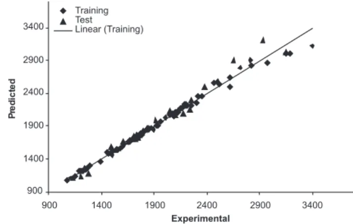
Figure 3. Agreement between predicted RI values and experimental values by L-M ANN
Topological descriptors are based on a graph representation of the molecule. They are numerical quantiiers of molecular topology obtained by the application of algebraic operators to matrices repre-senting molecular graphs and whose values are independent of vertex numbering or labeling. They can be sensitive to one or more structural features of the molecule such as size, shape, symmetry, branching and cyclicity and can also encode chemical information concerning atom type and bond multiplicity. Balaban index is a variant of connectivity index, represents extended connectivity and is a good descriptor for the shape of the molecules and modifying biological process. Nevertheless, some of chemists have used this index successfully in developing QSPR/QSRR models.
The radial distribution function descriptors are based on the distances distribution in the geometrical representation of a molecule and constitute a radial distribution function code. Formally, the radial distribution function of an ensemble of N atoms can be interpreted as the probability distribution of inding an atom in a spherical volume of radius r.38
L-M ANN analysis
With the aim of improving the predictive performance of nonli-near QSRR model, L-M ANN modeling was performed. Descriptors of GA-KPLS model were selected as inputs in L-M ANN model. The network architecture consisted of ive neurons in the input layer corresponding to the ive mentioned descriptors. The output layer had one neuron that predicts the RI. The number of neurons in the hidden layer is unknown and needs to be optimized. In addition to the number of neurons in the hidden layer, the learning rate, the momentum and the number of iterations also should be optimized. In this work, the number of neurons in the hidden layer and other parameters except the number of iterations were simultaneously optimized. A Matlab program was written to change the number of neurons in the hidden layer from 2 to 7, the learning rate from 0.001 to 0.1 with a step of 0.001 and the momentum from 0.1 to 0.99 with a step of 0.01. The root mean square errors for training set were calculated for all of the possible combination of values for the mentioned variables in cross validation. It was realized that the RMSE for the training set are mi-nimum when three neurons were selected in the hidden layer and the learning rate and the momentum values were 0.5 and 0.2, respectively. Finally, the number of iterations was optimized with the optimum values for the variables. It was realized that after 13 iterations, the RMSE for prediction set were minimum. The statistical parameters for L-M ANN model in Table 3. Plots of predicted RI versus expe-rimental RI values by L-M ANN are shown in Figure 3. Obviously, there is a close agreement between the experimental and predicted RI and the data represent a very low scattering around a straight line with respective slope and intercept close to one and zero. The closeness of the data to the straight line with a slope equal to 1 shows the perfect it of the data to a nonlinear model. It should be noted that the data shown in Figure 3 are the predicted values according to leave-group-out cross-validation and a deviation from the regression line is expected for some points. The Q2, which is a measure of the
model it to the cross validation set, can be calculated as:
(15)
where yi, yî and y
- were respectively the experimental, predicted, and
mean RI values of the samples. The accuracy of cross validation re-sults is extensively accepted in the literature considering the Q2 value.
In this sense, a high value of the statistical characteristic (Q2 > 0.5)
is considered as proof of the high predictive ability of the model.39
However, several authors suggest that a high value of Q2 appears to
be a necessary but not suficient condition for a model to have a high predictive power and consider that the predictive ability of a model can only be estimated using a suficiently large collection of compounds that was not used for building the model.40
We believe that applying only LGO-CV is not suficient to evalu-ate the predictive ability of a model. Thus we employed a two-step validation protocol which contains internal (LGO-CV) and external (test set) validation methods. The data set was randomly divided into training (calibration and prediction sets) and test sets after sorting based on the RI values. The training set consisted of 92 molecules and the test set, consisted of 24 molecules. The training set was used for model development, while the test set in which its molecules have no role in model building was used for evaluating the predictive ability of the models for external set. We reported that the retention index of this essential oil was mainly controlled by constitutional descriptors, functional groups and electronic descriptors.
The statistical parameters obtained by LGO-CV for L-M ANN, GA-KPLS and the linear QSRR models are compared in Table 3. In-spections of the results of this table reveals a higher R2 and Q2 values
and lower the RE for L-M ANN model for the training and test sets compared with their counterparts for GA-KPLS and other models. Moreover, the low values of root-mean-square error of prediction for the samples in the test set conirm the prediction ability of the resulted models for the compounds that were not used in the model-building step. In comparison with the plot of other models, the L-M ANN pre-dicted RI of each one of the training and test sets compound represent a uniform and linear distribution. This clearly shows the strength of L-M ANN as a nonlinear feature selection method. The key strength of L-M ANN is their ability to allow for lexible mapping of the selected features by manipulating their functional dependence implicitly. Neural network handles both linear and nonlinear relationship without adding complexity to the model. This capacity offset the large computing time required and complexity of L-M ANN model with respect other models.
CONCLUSION
was developed by employing the two linear models (GA-MLR and GA-PLS) and two nonlinear models (GA-KPLS and L-M ANN). The most important molecular descriptors selected represent the constitu-tional descriptors, funcconstitu-tional group and electronic descriptors that are known to be important in the retention mechanism of essential oils. Four models have good predictive capacity and excellent statistical pa-rameters. A comparison between these models revealed the superiority of the GA-KPLS and L-M ANN to other models. It is easy to notice that there was a good prospect for the GA-KPLS and L-M ANN ap-plication in the QSRR modeling. This indicates that the RI of essential oils possesses some nonlinear characteristics. In comparison with two nonlinear models, the results showed that the L-M ANN model can be effectively used to describe the molecular structure characteristic of these compounds. It can also be used successfully to estimate the RI for new compounds or for other compounds whose experimental values are unknown.
REFERENCES
1. Vagionas, K.; Ngassapa, O.; Runyoro, D.; Graikou, K.; Gortzi, O.; Chinou, I.; Food Chem.2007, 105, 1711.
2. Kim, N. S.; Lee, D. D.; J. Chromatogr., A2002, 982, 31.
3. Eminagaoglu, O.; Tepe, B.; Yumrutas, O.; Akpulat, H. A.; Daferera, D.; Polissiou, M.; Sokmen, A.; Food Chem.2007, 100, 339.
4. Radulović, N.; Lazarević, J.; Ristić N.; Palić R.; Biochem. Syst. Ecol.
2007, 35, 196.
5. Kotsos, M. P.; Aligiannis, N.; Mitakou, S.; Biochem. Syst. Ecol.2007, 35, 381.
6. Peters, R.; Tonoli, D.; van Duin, M.; Mommers, J.; Mengerink, Y.; Wil-bers, A. T. M.; van Benthem, R.; de Koster, Ch.; Schoenmakers, P. J.; van derWal, Sj.; J. Chromatogr., A2008, 1201, 141.
7. Li, Z. G.; Lee, M. R.; Shen, D. L.; Anal. Chim. Acta2006, 576, 43. 8. Acevedo-Martınez, J.; Escalona-Arranz, J. C.,; Villar-Rojas, A.;
Tellez-Palmero, F.; Perez-Roses, R.; Gonzalez, L.; Carrasco-Velar, R.; J. Chromatogr., A 2006, 1102, 238.
9. Teodora, I.; Ovidiu, I.; J. Mol. Design2002, 1, 94.
10. Ghasemi, J.; Saaidpour, S.; Brown, S. D.; J. Mol. Struct.2007, 805, 27. 11. Qin, L. T.; Liu, Sh. Sh.; Liu, H. L.; Tong, J.; J. Chromatogr., A2009,
1216, 5302.
12. Riahi, S.; Pourbasheer, E.; Ganjali, M. R; Norouzi, P.; J. Hazard. Mater.
2009, 166, 853.
13. Bombarda, I.; Dupuy, N.; Le Van Da, J. P.; Gaydou , E. M.; Anal. Chim. Acta2008, 613, 31.
14. Deeb, O.; Hemmateenejad, B.; Jaber, A.; Garduno-Juarez, R.; Miri, R.;
Chemosphere2007, 67, 2122.
15. Hemmateenejad, B.; Miri, R.; Akhond, M.; Shamsipur, M.; Chemom. Intell. Lab. Syst. 2002, 64, 91.
16. Kim, K.; Lee, J. M.; Lee, I. B.; Chemom. Intell. Lab. Syst. 2005, 79, 22. 17. Rosipal, R.; Trejo, L. J.; J. Mach. Learning Res. 2001, 2, 97. 18. Haykin, S.; Neural Networks, Prentice-Hall: New Jersey, 1999. 19. Conforti, F.; Menichini, F.; Formisano, C.; Rigano, D.; Senatore, F.;
Arnold, N. A.; Piozzi, F.; Food Chem. 2009, 116, 898.
20. Todeschini, R.; Consonni, V.; Mauri, A.; Pavan, M.; DRAGON-Software for the calculation of molecular descriptors; Version 3.0 for Windows, 2003.
21. Cai, W.; Xia, B.; Shao, X.; Guo, Q.; Maigret, B.; Pan, Z.; J. Mol. Struct. 2001, 535, 115.
22. Goldberg, D. E.; Genetic Algorithms in Search, Optimization and Ma-chine Learning, Addison-Wesley–Longman: Reading, 2000.
23. Depczynski, U.; Frost, V. J.; Molt, K.; Anal. Chim. Acta2000, 420, 217. 24. Citra, M.; Chemosphere1999, 38, 191.
25. Hemmateenejad, B.; Shamsipur, M.; Miri, R.; Elyasi, M.; Foroghinia, F.; Sharghi, H.; Anal. Chim. Acta2008, 610, 25.
26. Wold, S.; Sjostrom, M.; Eriksson, L.; Chemom. Intell. Lab. Syst.2001,
58, 109.
27. Tang, K.; Li, T.; Anal. Chim. Acta2003, 476, 85.
28. Rosipal, R.; Trejo, L. J.; J. Mach. Learning Res. 2001, 2, 97.
29. Zupan, J.; Gasteiger, J.; Neural Network in Chemistry and Drug Design, Wiley–VCH: Weinheim, 1999.
30. Beal, T. M.; Hagan, H. B.; Demuth, M.; Neural Network Design, PWS: Boston, 1996.
31. Zupan, J.; Gasteiger, J.; Neural Networks for Chemists: An Introduction, VCH: Weinheim, 1993.
32. Guven, A.; Kara, S.; Exp. Sys. Appli. 2006, 31, 199.
33. Salvi, M.; Dazzi, D.; Pelistri, I.; Neri, F.; Wall, J. R.; Ophthalmology
2002, 109, 1703.
34. Kim, K.; Lee, J. M.; Lee, I. B.; Chemom. Intell. Lab. Syst. 2005, 79, 22. 35. Booth, T. D.; Azzaoui, K.; Wainer, I. W.; Anal. Chem. 1997, 69, 3879. 36. Yu, X.; Yi, B.; Liu, F.; Wang, X.; React. Funct. Polym. 2008, 68, 1557. 37. Karelson, M.; Molecular descriptors in QSAR/QSPR,
Wiley-Interscience: New York, 2000.
38. Todeschini, R.; Consonni, V.; Handbook of molecular descriptors, Wiley-VCH: Weinheim, 2000.
39. Hemmateenejad, B.; Javadnia, K.; Elyasi, M.; Anal. Chim. Acta2007,
592, 72.