Modeling the Mutualistic Interactions
between Tubeworms and Microbial Consortia
Erik E. Cordes
1*, Michael A. Arthur
2, Katriona Shea
1, Rolf S. Arvidson
3, Charles R. Fisher
11Biology Department, Pennsylvania State University, University Park, Pennsylvania, United States of America, 2Geosciences Department, Pennsylvania State University, University Park, Pennsylvania, United States of America, 3Department of Earth Science, Rice University, Houston, Texas, United States of America
The deep-sea vestimentiferan tubeworm
Lamellibrachia luymesi
forms large aggregations at hydrocarbon seeps in the
Gulf of Mexico that may persist for over 250 y. Here, we present the results of a diagenetic model in which tubeworm
aggregation persistence is achieved through augmentation of the supply of sulfate to hydrocarbon seep sediments. In
the model,
L. luymesi
releases the sulfate generated by its internal, chemoautotrophic, sulfide-oxidizing symbionts
through posterior root-like extensions of its body. The sulfate fuels sulfate reduction, commonly coupled to anaerobic
methane oxidation and hydrocarbon degradation by bacterial–archaeal consortia. If sulfate is released by the
tubeworms, sulfide generation mainly by hydrocarbon degradation is sufficient to support moderate-sized
aggregations of
L. luymesi
for hundreds of years. The results of this model expand our concept of the potential
benefits derived from complex interspecific relationships, in this case involving members of all three domains of life.
Citation: Cordes EE, Arthur MA, Shea K, Arvidson RS, Fisher CR (2005) Modeling the mutualistic interactions between tubeworms and microbial consortia. PLoS Biol 3(3): e77.
Introduction
Complex positive species interactions have been shown to
expand the ecological niche and increase the persistence of
the organisms involved in a variety of systems. In terrestrial
systems, increased diversity of mycorrhizal symbionts is
correlated with increased biodiversity of plant communities,
resulting in greater stability and longer persistence at the
community level [1]. In marine ecosystems, the coral
Oculina
arbuscula
harbors a majid crab,
Mithrax forceps,
that prevents
overgrowth of macroalgae and shading of the corals [2]. This
allows
O. arbuscula
to maintain its facultative mutualism with
photosynthetic zooxanthellae in well-lit habitats off the
Atlantic coast of North Carolina, increasing the amount of
energy available to the coral for growth and reproduction. At
cold seeps in the Cascadia [3,4] and Aleutian [5] subduction
zones, bioirrigation through burrow formation and
biotur-bation by clams (Calyptogena
spp.) has been shown to
significantly affect the distribution of microbial anaerobic
methane oxidation.
Lamellibrachia luymesi
inhabits areas associated with
advec-tion of hydrocarbons and other reduced chemicals to the
seafloor (hydrocarbon or brine seeps) on the upper Louisiana
slope (ULS) of the Gulf of Mexico from 400 to 1,000 m depth.
L. luymesi
does not posses a digestive system; rather, it acquires
energy via internal sulfide-oxidizing bacterial symbionts [6].
L. luymesi
differs from other vestimentiferan tubeworms by its
ability to use a posterior extension of its body, the
‘‘
root,
’’
to
acquire sulfide from interstitial pools in sediments [7,8]. Near
the anterior plumes of tubeworms, sulfide concentrations
typically decline below 0.1
lM as the tubeworms approach 1 m
in length [9]. By using its roots,
L. luymesi
is able to delve into
deeper sediment layers, providing access to more persistent
sulfide sources. In the apparent absence of lethal predation
[10,11], the most significant hazard that this vestimentiferan
tubeworm faces is sulfide limitation. Its high uptake rate of
sulfide from hydrocarbon seep sediments, estimated at over 30
lmol
h
1for a moderate-sized individual [12], suggests that
sulfide flux may be limiting in
L. luymesi’s habitat.
A diverse chemosynthetic community relies on the sulfide
generated as a by-product of anaerobic degradative
pro-cesses in the Gulf of Mexico [10,11]. Reduction of seawater
sulfate utilizing methane or other hydrocarbons as electron
donors produces the majority of sulfide available at ULS
seeps [13,14]. Anaerobic methane oxidation is most
com-monly carried out by microbial consortia consisting of
sulfate-reducing bacteria along with methanogenic archaea
executing reverse methanogenesis [15,16]. Methane oxidation
linked to sulfate reduction and subsequent authigenic
carbonate precipitation constrain ocean–atmosphere carbon
fluxes [3,4], accounting for up to 20% of the global methane
flux to the atmosphere [17]. Oxidation of other hydrocarbons
and organic material, carried out by sulfate-reducing
bacteria in monoculture and in consortia with other
microbes [18], may account for a larger proportion of sulfate
depletion in ULS sediments [14]. These processes can result
in a decoupling of sulfate reduction and methane oxidation
rates [14], and form carbonates consisting mainly of
non-methane-derived carbon [19].
L. luymesi
may influence these
anaerobic processes by utilizing its roots to release the
sulfate generated by its symbionts during sulfide oxidation
[7,8,12]. This hypothetical mechanism would provide sulfate
for anaerobic methane oxidation and hydrocarbon
degrada-tion at sediment depths normally devoid of energetically
favorable oxidants, thereby augmenting exogenous sulfide
production.
Received July 5, 2004; Accepted December 23, 2004; Published February 22, 2005 DOI: 10.1371/journal.pbio.0030077
Copyright:Ó2005 Cordes et al. This is an open-access article distributed under the terms of the Creative Commons Attribution License, which permits unrestricted use, distribution, and reproduction in any medium, provided the original work is properly cited.
Abbreviations: DIC, dissolved inorganic carbon; DOC, dissolved organic carbon ULS, upper Louisiana slope
Academic Editor: Robert C. Vrijenhoek, Monterey Bay Aquarium Research Institute, United States of America
In this study, we address the question of whether known
biogeochemical processes could supply sulfide at rates
sufficient to match the requirements of long-lived
L. luymesi
aggregations. In the diagenetic model presented here, the
hypothesized release of sulfate in sediments with sufficient
electron donors results in sulfide generation at rates
matching the sulfide uptake rate of
L. luymesi
aggregations
for over 250 y. We speculate that the mutual benefits derived
from the syntrophy among symbiotic tubeworms and
micro-bial consortia implicit in the model would expand our
current concept for the potential complexity of positive
interspecific interactions and the benefits they confer.
Results/Discussion
L. luymesi
Sulfate Release Allows Persistence of
Aggregations
The model predicts that inputs from known sources,
including diffusion and advection of deep sulfide along with
reduced seawater sulfate, will support a moderately-sized
aggregation of 1,000 individuals for an average of 39 y (range,
22 to 78 y) (Figure 1). A smaller aggregation of 200 individuals
could be maintained with these sources for an average of 64.1
y (standard deviation, 10.6 y). In this model configuration, the
duration of adequate sulfide flux is not congruent with the
known sizes of aggregations and existing age estimates of
L. luymesi
individuals and aggregations. Adding sulfate release
by tubeworm roots to the model results in sulfide generation
and flux at rates that match the demands of large
aggregations, allowing the tubeworms to survive for over
250 y (Figure 1). This additional source of sulfate results in a
two-orders-of-magnitude increase in sulfate flux in older
(
.
100 y) aggregations, accounting for over 90% of sulfate
available after only 24 y. The sulfate released by the
tubeworms would be used for anaerobic methane oxidation
and hydrocarbon degradation. The nature of the relationship
between symbiotic tubeworms and microbial consortia that
we are proposing is a coupling of the sulfur cycle only, and
not carbon. Light dissolved inorganic carbon (DIC) resulting
from the oxidation of hydrocarbons is apparently not taken
up by tubeworms as the carbon stable isotope signatures of
L. luymesi
are heavier than would be expected from a
methane-derived DIC source [20,21]. In addition, the
well-studied hydrothermal vent tubeworm,
Riftia pachyptila,
ob-tains carbon in the form of CO
2across its plume [22].
However, this does not necessarily exclude the passive
diffusion of DIC across the root surface, which could account
for some of the variability observed in
L. luymesi
carbon stable
isotope signatures [20,21]. By augmenting the sulfate supply
to microbial consortia for sulfate reduction, large
aggrega-tions of tubeworms may survive for hundreds of years in the
model, mirroring the population sizes and individual lengths
regularly observed and collected at seeps on the ULS [23].
Model Results Are Robust to Parameter Variation
An alternate hypothesis to explain the discordance
between estimated sulfide supply and uptake rates is the
presence of locally elevated seepage rates. Sensitivity analyses
were carried out to determine the potential effects of
uncertainty in seepage rate on supply estimated for
aggrega-tions without root sulfate release. A 10% increase in seepage
rate resulted in a 5.6% increase in sulfide supply to
aggregations 200 y old and older. This corresponds to only
16.4% of the sulfide required, which does not serve to extend
aggregation survivorship (average, 39 y; range, 21 to 79 y)
beyond that determined for lower flow rates. To supply the
sulfide flux required by older aggregations, seepage rate
would have to be at least 363 mm
y
1. This is over ten times
greater than the rate used in the model (32 mm
y
1), which is
the highest region-wide estimate for the Gulf of Mexico [24].
A rate of over 300 mm
y
1approaches rates reported for
active venting of fluids (Table 1). Active venting would result
in the visual manifestation of seepage in the form of methane
bubbles and oil droplets, which are generally restricted to
mussel (Bathymodiolus childressi) beds at these sites [25]. In
addition, larger, and therefore older [26], aggregations have
lower epibenthic sulfide concentrations [8,9,25] suggesting
that seepage becomes less vigorous over time and is not in the
form of active venting in larger tubeworm aggregations.
While difficult to obtain, in situ measures of advection rate of
fluids at Gulf of Mexico seeps could be used to test these
assumptions and may lend insight into the relationship
between variability in tubeworm growth rate and sulfide
availability.
The high degree of variability in growth rate and
recruit-ment rate could also affect the ratio of supply and demand in
the model. In an aggregation exhibiting anomalously low
recruitment, the size of the rhizosphere would increase more
rapidly than the biomass of the aggregation. This would lead
to high rates of sulfide delivery and generation and low rates
of sulfide uptake by tubeworm roots. When initial
recruit-ment rate (a
in equations 1 and 2) is decreased by 10%, the
length of time that supply exceeds demand increases by 3.7%.
This effect appears to be linear, with a 20% decrease in initial
recruitment rate resulting in a 7.4% increase in persistence.
If growth rate is increased, thereby increasing the rate of
rhizosphere growth in terms of surface area for diffusion and
Figure 1.Ratio of Sulfide Supply to Sulfide Uptake Rate ofL. luymesiAggregations
Equilibrium line (1:1 ratio) and average, maximum, and minimum values for 1,000 iterations presented. Supply rate based on known sources without sulfate release by tubeworm roots shown in blue. Sulfide supply declines below demand after approximately 40 y. Supply rate including sulfate release from tubeworm roots shown in red, with sulfate release constrained by tubeworm symbionts’ sulfide oxidation rate. Sulfide supply exceeds demand for the duration of the model.
advection, there appears to be little effect of the ratio of
supply to demand (20% increase in growth—0% change in
persistence time). In fact, increasing growth to the upper
limits of the error term (equation 5) lowers the amount of
time that the aggregation can be supported since biomass and
sulfide demand increase more rapidly than increases in
supply resulting from additional surface area. By decreasing
growth rate, aggregations may be supported for longer
periods of time, with a 20% decrease leading to a 6.3%
increase in persistence time and a decrease of 88% leading to
persistence for over 250 y. While an 88% lower growth rate
lies outside of the range of existing growth data, this could be
accomplished by ceasing growth for extended periods of time
in a quiescent stage. This possibility remains to be
inves-tigated in
L. luymesi. By utilizing a variable recruitment rate in
the model, both between realized aggregations and between
years within a model run, along with a growth error term
encompassing the full range of observed growth data, the
model is capable of generating aggregations within the range
of the 10%–20% variability tested in this analysis. Even these
outlying aggregations (presented as maxima and minima in
Figure 1) support the qualitative conclusions drawn from
model results.
While the model was based on empirical data to the
greatest degree possible, estimates of many of the parameters
necessary to resolve the model were not available or are
extremely difficult to measure in deep water with existing
technology. Uptake rates were measured in the laboratory [8]
for relatively small individuals (
,
50 cm). While we attempted
to approximate metabolic scaling by covarying uptake and
growth rates, it is possible that large individuals require even
lower sulfide flux. Model predictions are not overly sensitive
to variability in this parameter. A reduction by 10% of the
overall sulfide uptake rate results in a 5.2% increase in
persistence time. To maintain an aggregation for over 250 y,
mass-specific uptake rate would have to be reduced 6-fold.
While this could also be accomplished by entering a period of
quiescence as mentioned before, there is no existing evidence
for this ability in vestimentiferans.
The second version of the model is based on the
assumption that
L. luymesi
is capable of releasing sulfate
through its roots. It should be noted that in the model, sulfate
release is constrained by the rate of sulfate generation by the
tubeworm’s sulfide-oxidizing symbionts, resulting in the near
1:1 ratio of supply and demand in Figure 1. Though modeled
sulfate flux across the roots into the rhizosphere may exceed
20 mmol
h
1in older aggregations, the roots provide an
ample respiratory surface such that rates of sulfate flux per
unit root surface area do not exceed 0.4
lmol
h
1cm
2in
the model. It remains possible that a proportion of the sulfate
could be released through the plume of the tubeworms,
though the energy required to pump sulfate against a
concentration gradient (seawater [SO
4] = 29 mM) [13]
suggests that it would be more energetically favorable for
the sulfate to passively diffuse out of the roots. It is also
possible that sulfate flux could be increased by active
bioirrigation delivering seawater to deeper sediment layers
through the tubeworm tubes. This could allow the
sulfide-oxidizing symbionts to store some of the oxidized sulfide as
elemental sulfur rather than releasing it as sulfate, while
maintaining sufficient sulfate flux to deeper sediment layers
for sulfide generation. These mechanisms remain
hypo-thetical and require further experimental investigations to
evaluate their potential role in this system.
Tubeworms Impact Seep Biogeochemistry
Tubeworm sulfate release, in conjunction with high sulfide
uptake rates, could contribute to the observation of declining
advection rate in older aggregations. By increasing sulfate
flux to deeper sediments,
L. luymesi
increases integrated rates
of anaerobic methane oxidation and hydrocarbon
degrada-tion, which would enhance authigenic calcium carbonate
precipitation within the rhizosphere. Under the conditions of
root sulfate release in the model, calcium carbonate
precipitation is rapid (0.109 to 0.316
lmol
l
1sec
1) in
the first 53 y, with rates declining exponentially thereafter. By
creating a barrier to fluid advection [4], this could result in
the observed decrease in epibenthic sulfide concentration in
older aggregations [8,9] and the predicted cessation of
tubeworm recruitment around this time [12,23].
In order to prevent the precipitation of carbonate directly
on the root surface,
L. luymesi
individuals may release
gen ions as well as sulfate through their roots. While
hydro-gen ion flux through the roots has not yet been empirically
demonstrated, none of the nearly 5,000 tubeworms examined
as part of this study were observed to have carbonate formed
directly on their roots, suggesting that this form of
precipitation is inhibited in some manner. In the model,
diffusion of hydrogen ions across the root surface (the only
form of release explicitly modeled) accounts for less than
40% of ion generation when carbonate precipitation is most
vigorous. We speculate that
L. luymesi
may utilize the excess
hydrogen ions generated by their sulfide-oxidizing symbionts
to periodically raise the rate of hydrogen ion flux from their
Table 1.
Reported Seepage Rates for Hydrocarbon and Methane
Seeps
Site Published Millimeters per Year
Notes and Source
Gulf of Mexico 1.4 m3/1,000 km2/d 1.5 Region-wide seepage [24] Gulf of Mexico 30 m3/1,000 km2/d 32 Region-wide seepage [24] Gulf of Mexico 7 km/1 My 7 Oil migration [53] Juan de Fuca 2 mm/y 2 ‘‘Strong upwelling’’[54] Juan de Fuca 4,000 m/My 4 Maximum of modeled
rates [54] Cascadia 51012m3/m2/s 0.26 Vertical compaction
model [55] Cascadia 106m3/m2/s 52,000 Measured at‘‘small’’
vent [55] Nankai 10 to 30 m/y 20,000 Temperature profiles
at active vent [56] Barbados 0.2 to 10 mm/y 5.1 Temperature profiles (Darcy Velocity) [57]
Barbados 6 cm/y 60 Temperature profiles
(Darcy Velocity) [57] Aleutians 3.4 m/y 3,400 To support benthic
oxygen flux [5] Eel River, CA 10 cm/y 100 In situ measurement [58] Indonesia 0.15 m/y 1,500 Expulsion of warm
fluids [59] Indonesia 3.1105
m/y 0.31 ‘‘Marginal area’’near vent [59]
— 1 kg/m2/y 1.61 Theoretical [60]
roots. This would not only supply additional hydrogen ions to
sulfate-reducing bacteria, but could inhibit carbonate
pre-cipitation on the tubes and subsequent reduction of the root
area utilizable as a respiratory surface. Further pH reduction
could dissolve existing carbonate in sediments beneath the
rhizosphere, thereby opening seepage pathways and allowing
further root growth. This possibility is corroborated by the
observation of young tubeworms that had apparently bored
through bivalve shells in an experimental system (R. Carney,
personal communication). Empirical measurements of
hydro-gen ion flux across the root tissue of
L. luymesi
are required to
test these hypothetical mechanisms.
The release of sulfate by tubeworm roots potentially
explains the frequent observation of highly degraded
hydro-carbons in the vicinity of large tubeworm aggregations [27].
The majority of sulfate supplied by tubeworm roots is utilized
for microbial hydrocarbon degradation in the model
(Figure2). This process alone accounts for over 60% of the
sulfide available to aggregations after approximately 80 y. In
the absence of liquid and solid phase hydrocarbons, methane
flux would have to be approximately four times the rate in
the model in order to fuel sufficient sulfate reduction to
support an aggregation for over 200 y. This could occur in
sediments overlying rapidly sublimating gas hydrates, and
hydrate abundance has been previously suggested as a
potential factor influencing the distribution of
chemosyn-thetic communities in the Gulf of Mexico [10]. However,
model results indicate that large chain hydrocarbons are the
most significant energy source for sulfate reduction in
tubeworm-dominated sediments. Increased integrated rates
of hydrocarbon degradation would lead to highly biologically
altered hydrocarbon pools among the roots of tubeworm
aggregations. Hydrocarbon oxidation has been implicated as
one of the dominant processes in the carbon cycle at ULS
seeps, accounting for over 90% of the carbon in carbonates
collected in the vicinity of tubeworm aggregations [19].
Model analysis indicates that the minimum amount of
organic carbon (including hydrocarbons as well as buried
organic material) in sediments required to supply sulfide at
rates matching aggregation demand (1:1 supply:uptake ratio)
is 1.03% by weight, remarkably close to the lowest value
found in any of the seep sediment core samples (1.2%)
[13,28], and greater than that found in ULS sediments away
from seeps (0.71%) [29]. Determination of organic carbon
concentration in sediments beneath tubeworm aggregations
is necessary to test the prediction that elevated carbon
content at seeps, primarily resulting from oil seepage,
provides the energy source required to generate sufficient
sulfide for tubeworm aggregations.
Additional sulfate flux from tubeworm roots could also
explain the high apparent sulfate diffusion coefficients
determined for tubeworm-impacted sediments [13].
Anom-alous sulfate fluxes have been proposed to be a result of
bioturbation and bioirrigation by macrofauna [3,5], and
recycling by microbial mats [13]. The results of the model
presented here provide evidence for macrofaunal sulfur
recycling, an additional component to be considered in
future investigations of cold seep biogeochemistry. The
hypothesized release of sulfate by tubeworm roots potentially
explains numerous, apparently disparate observations,
hint-ing at the great impact that
L. luymesi
aggregations may have
on their abiotic environment.
While the proposed interactions between symbiotic
tube-worms and sulfate-reducing bacteria are essential for the
persistence of
L. luymesi
aggregations in the model, we suggest
that there are significant effects on the microbial community
as well. This syntrophy will increase the abundance of
sulfate-reducing bacteria and therefore increase the rates of
anaerobic methane oxidation and hydrocarbon degradation
carried out by microbial consortia that rely on sulfate as an
oxidant. Tubeworm-generated sulfate supplies a more
en-ergetically favorable electron acceptor below the normal
depth of sulfate penetration at seeps, relaxing the limitation
on anaerobic oxidative processes at these sediment depths.
Deeper sediment layers then become habitable to sulfate
reducers, significantly altering the microbial community
structure within the rhizosphere. Model configurations
neglect the potential role of bioirrigation of seawater sulfate
through
L. luymesi
tubes, which could further increase sulfate
supply to deeper sediment layers. The possible role of
tubeworm roots as substrata for the growth of microbial
consortia, analogous to the habitat afforded mycorrhizal
symbionts of higher plants, remains another possible benefit
for the microbes. These predictions may be tested by
determination of the relative abundance of microbial
consortia at different depths of sediments both impacted by
and isolated from tubeworms. Localization of the microbes
on the root surface would provide evidence for a more
intricate relationship. It is our hope that the results of this
model may provide the impetus for future rigorous
exper-imental tests of these ideas.
Summary
The model results presented here are consistent with the
hypothesis that
L. luymesi
releases sulfate into
hydrocarbon-rich sediments to fuel sulfide generation, allowing for the
persistence of the longest-lived animal known. The
impor-tance of this process to sulfide generation in the modeled
rhizosphere implies a complex relationship between an animal
Figure 2.Sources of Sulfide Available to Tubeworm Aggregations overTime in the Model
Sources of sulfide include advection and diffusion of sulfide from deep sources (yellow) or sulfate reduction using methane (blue), buried organic carbon (green), or C6þhydrocarbons (dark grey) as
electron donors. Sulfate is provided by diffusion from sediments surrounding the rhizosphere, diffusion at the sediment–water inter-face, and release from tubeworm roots.
with bacterial endosymbionts and external sulfate-reducing
bacteria, often in consortia with methane-oxidizing or
hydro-carbon-degrading microbes. This positive interspecific
rela-tionship, including members of all three domains, would
benefit both the tubeworms and the microbial consortia
involved. This expands our existing concept of the potential
for complexity in mutualisms and the benefits they may confer.
Further complex relationships are likely to be discovered
through continued research into the role of positive species
interactions at the individual and community levels.
Materials and Methods
This study couples an individual-based population growth and sulfide uptake model [12] to a diagenetic diffusion/advection model to compare the relative magnitude of sulfide supply and uptake for long-lived tubeworm aggregations. A series of 1,000 iterations of the model under three different initial conditions (known sources of sulfate, known sources plus root sulfate supply, and known sources with elevated seepage rates) were carried out. The rhizosphere (volume of sediment encompassed by the root system of an aggregation) is modeled as an inverted dome beneath the sediment with a radius equal to the average root length of the population (Figure 3). The rhizosphere was approximated by a series of two-dimensional discs at 2-cm intervals in order to reduce the complexity of a three-dimensional solution for a sphere of changing size. Sulfate (SO42), methane (CH4), sulfide (HS), bicarbonate (HCO3), and hydrogen ion (Hþ) fluxes across the rhizosphere boundary are
determined. Sulfate reduction rates using methane, larger chain hydrocarbons, and buried organic matter as electron donors are modeled in order to estimate the sulfide available to tubeworm aggregations as they change in size over the course of 250 y.
Population growth model.The population growth model follows the methodology presented in [12] and includes population growth, mortality rate, individual growth rate, and sulfide uptake rate. The parameters underlying the population growth model were refined using growth data from an additional 615 individuals and population data from an additional 11 aggregations comprising 4,908 individuals. The model presented here includes data from a total of 23 tubeworm aggregations from three nearby sites (Green Canyon oil lease blocks 184, 232, and 234) collected over a period of 7 y on the ULS to arrive at generalized population growth parameters.
L. luymesiindividuals are dioecious, with males releasing sperm into the water column. Fertilization is believed to be external [30], though sperm has been found within the oviducts of females of the hydrothermal vent tubewormR. pachyptila [31]. Eggs and embryos are positively buoyant and develop into a swimming trochophore-like larval stage within 3 d of fertilization [32]. Larvae are lecithotrophic and may remain in the water column for several weeks [32]. They require hard substrata for settlement, and acquire symbionts from their environment after metamorphosis [33,34]. Settlement is initially rapid, and continues until the available substrate is occupied [12,23,35]. Population sizes of aggregations collected with existing sampling devices typically vary between 100 and 1,500 individuals ([12,23]; this study), though far larger aggregations covering tens to hundreds of square meters are common at the sites sampled. Previous studies have shown thatL. luymesihas an average longevity of 135 y [12], and requires an average of 210 y to reach 2 m in length [26], a size not uncommon among collected animals. Mortality events are exceedingly rare, dropping below 1% annual mortality probability for animals over 30 cm [12]. The expanded datasets of growth and mortality rates included here extend the longevity estimate for L. luymesito an average of 176 y and the estimated age of a 2-m-long animal to 216 y.
At the beginning of each iteration, population growth parameters are chosen for the following population growth model:
dN dt¼
aN 1þbaN
K
c ð1Þ
whereNis population size,tis time (in years),Kis carrying capacity (set to 1,000 individuals for all simulations presented here), a describes the initial slope of the line,bdefines the degree of density dependence, andcis a shape parameter. The first parameter(a)was generated using the following function:
a¼0:7451þ ð0:444e½Nð0;1ÞÞ ð2Þ
where e[N(0,1)] is a normally distributed random deviate with an average of zero and a standard deviation of one. This allows the initial recruitment rate to vary within the range of all recruitment trajectories that have been observed [12]. The other parameters were not normally distributed; therefore, the log-transformed distribu-tions were used to define the distribution of the random numbers generated. As the three parameters in the model were significantly correlated (ln(a) and ln(b),r =0.853, p, 0.001; ln(a) and ln (c), r =0.461,p= 0.036), values of b andcwere chosen from their relationship witha:
lnðbÞ ¼ 6:5309lnðaÞ þ3:4174 ð3Þ
lnðcÞ ¼ 0:3789lnðaÞ þ1:3561 ð4Þ
The value ofawas allowed to vary each year according to the pooled standard error associated with the estimates ofafrom the empirical data (standard error, 0.105). Once population size equaled or exceeded carrying capacity, recruitment was ceased, representing the lack of additional substrate or sulfide available in the water column.
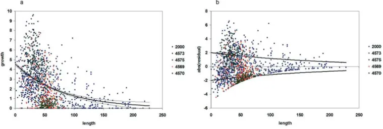
Once recruitment was determined for that year, the individual-based portion of the model began. Each individual was traced through time with respect to its length, root length, mass, mortality probability, mass-specific sulfide uptake rate, sulfate excretion rate, and hydrogen ion elimination rate. Growth rates of tubeworms were determined by staining tubes in situ (Figure 3) and collection 12 to 14 mo later ([26]; this study). Individual growth rate was determined from the following function (Figure 4):
dl dt¼4:554e
0:01269l6ð2
:007e
0:00537le½Nð0
;1ÞÞ ð5Þ
Length(l)is defined here as the distance from the anterior end of the tube to an outer tube diameter of 2 mm following the methodology of [26]. All growth rates were standardized to 365 d. The error term is an additional function fitted to the residuals of the first regression function (Figure 4B), resulting in a variable growth rate. This error term was used rather than varying growth within the 95% confidence interval of the regression of length and growth rate because of the Figure 3.Model Construction
Population model includes individual size-specific growth and mortality rates, and population size-specific recruitment rate. Growth rate was determined by in situ staining of tubeworm aggregations using a blue chitin stain (in situ photograph of stained aggregation demonstrating annual growth shown here) and collection after 12–14 mo. Diagenetic model included advection and diffusion of sulfate, sulfide, methane, bicarbonate, and hydrogen ions as well as organic carbon content of sediments. Fluxes across the rhizosphere (root system) boundary were compared to sulfide uptake rates for simulated aggregations to determine whether sulfide supply could match the required uptake rates of aggregations (for specific methodology see methods). HC, C6þ hydrocarbons; orgC, organic
high degree of variability in growth among individuals. It should also be noted that there is a certain degree of variability in growth rate between aggregations (Figure 4). This may be attributable to spatial or temporal variability in seepage rate or sulfide concentration between aggregations. Aggregations may be subject to persistently differing conditions on a small (meter) scale, or may encounter periodic fluctuations in habitat characteristics. Because we are uncertain whether this variation is persistent on the temporal scales that we are simulating, between-aggregation variability is not ex-plicitly modeled, though by chance certain realized aggregations deviated from mean growth rate.
The ratio of root length to tube length was determined from individual length using the following function:
r:s¼6:134l
0:7024þ1
:0 ð6Þ
Annual mortality rate was approximated as the size-specific frequency of empty tubes in collected aggregations [12] with an overall annual mortality rate of 0.569%. This approximation is conservative and likely overestimates yearly mortality, as available data indicate that empty tubes should persist longer than 1 y [12,36]. Mortality probability was determined for each 10-cm size class using the following function:
m¼0:0298e
0:0446l ð7Þ
wherem is mortality probability and l is length. Individuals were considered dead if their probability of mortality exceeded a uniform random number between zero and one.
By using generalized population growth parameters in the model presented here, we attempt to encompass the range of empirical data from sampled aggregations in our examination of sulfide uptake and supply rates. Taken together, the population growth model including recruitment, growth, and mortality provides a good qualitative if not quantitative fit for any individual aggregation, reflecting the size frequency of tubeworms within sampled aggregations [12]. It should be noted that the modeling of specific aggregations was not the aim of this study; rather, an attempt has been made to encompass the variability observed in the various populations of tubeworms that have been sampled. To examine the effect of uncertainty in the population growth parameters, sensitivity analyses were carried out. The initial slope of the recruitment rate (ain equation 1) was varied while individual size-specific growth rate was held constant (no error term in equation 5). Growth rate was then varied while holding the initial rate of population growth constant (no error term in equation 2). The effect of a 10% change in each parameter was determined, and then changes of greater magnitude were examined to determine the fastest rate of population or individual growth that could be supported by the sulfide available to the aggregation in the absence of sulfate release.
Individual sulfide uptake was allowed to vary within the range of laboratory-determined sulfide uptake rates according to that indi-vidual’s growth rate for that year:
u¼m 1:60þ4:40
g 10
h i
ð8Þ
whereuis uptake rate (in micromoles per gram per hour),mis mass (in grams), andgis growth rate (in centimeters per year). Growth rate was divided by the maximum growth rate (10 cm y1) such that highest growth rates resulted in highest uptake rates. By scaling uptake rate with growth, we approximate metabolic scaling, resulting in a decline in uptake rate by a factor of 3.7 over the range of tubeworm sizes in this study [12]. The amount of sulfate that could be excreted by each individual was determined from the amount generated by sulfide oxidation carried out by the internal chemo-autotrophic symbionts assuming constant internal sulfate concen-tration, thereby accounting for changes in body volume. We do not account for the binding of sulfur by free amino acids, as this is believed to relatively minor compared the flux rates of sulfate and sulfide, and is reversible [37]. Hydrogen ions are also generated in the oxidation of sulfide by the tubeworm symbionts. Hydrogen ion elimination rate was determined in the model in the same fashion as sulfide uptake, with growth rate determining the variability in this metabolic flux according to laboratory-measured ion fluxes (mean, 10.96lmolg1h1; standard deviation, 1.88lmolg1h1) [38]. Simple diffusion of hydrogen ions across the root surface was included in the model, though the exact mode of proton flux has not yet been determined experimentally forL. luymesi[38]. As diffusion across the roots accounts for a relatively small proportion of total proton flux (less than 10% in large individuals), additional pathways are likely and require further investigation.
Geochemical setting. Known sources of sulfide available to L. luymesi aggregations are sulfide transported with seeping fluids [10] and sulfide generated via reduction of seawater sulfate [39,40]. The majority of the sulfide present at ULS sites is believed to be related to sulfate reduction coupled to anaerobic hydrocarbon oxidation [14,39]. Other potential sources of sulfide associated with seepage include anaerobic oxidation of deeply buried organic material [10],‘‘sour’’hydrocarbons containing a proportion of sulfur [41], and hydrocarbon interactions with sulfur-bearing minerals such as gypsum and anhydrite found in the salt dome cap rocks of the ULS [8,42,43].
Concentrations of all chemical species in the sediments surround-ing the rhizosphere were derived from the dataset included in Arvidson et al. [13] and Morse et al. [28]. Only those sediment cores taken around the ‘‘drip line’’ of tubeworm aggregations that contained detectable sulfide concentrations were used. Due to the vagaries of sampling with a submersible in sediments heavily impacted by carbonate and roots, those cores with detectable sulfide
Figure 4.L. luymesiGrowth Rate
Size-specific growth ofL. luymesidetermined from stained tubeworms. Different colors indicate growth data from different aggregations. Blue points labeled‘‘2000’’are all from Bergquist et al. [26]. Other colored points refer to submersible dive numbers from 2003 when stained aggregations were collected.
(A) Growth function and 95% confidence interval for size-specific growth. (B) Error function fitted to the residuals of the model.
are believed to more accurately represent conditions around the periphery of the rhizosphere.
Dissolved organic carbon (DOC) concentration was used as an estimate of methane concentration. While other forms of DOC make up this total concentration, methane accounts for 90%–95% of the hydrocarbon gasses dissolved in pore waters [28]. In seep sediments, the majority of DOC is likely to be in the form of hydrocarbon gasses. Because estimates of organic acid concentrations were not available, they could not be explicitly modeled. This would not affect the overall concentration of electron donors in the model, but could affect the sulfate reduction rate. Since sulfate reduction rate estimates for methane seeps in the Gulf of Mexico are among the highest recorded [14,39], any differences in DOC composition (e.g., higher relative concentrations of dissolved organic acids) would serve to lower the overall sulfate reduction rate and sulfide availability. Sulfide supply estimates presented are likely overestimated most by the model without root sulfate release owing to the greater reliance on anaerobic methane oxidation in this form of the model. Simulations including sulfate release by tubeworms are affected to a lesser extent as the concentration of electron donors is not limiting in this model configuration.
Solid and liquid phase organic carbon was separated into hydro-carbons and buried organic material according to their relative concentrations in hydrocarbon seep and surrounding Gulf of Mexico sediments. Background sediments on the ULS contain 0.71% organic carbon by weight [29]. At hydrocarbon seeps on the ULS, organic carbon accounts for 4.47% of total weight. This was assumed to be the sum of background organic input plus carbon in the form of C6þ
hydrocarbons. It is possible that the higher biomass located at ULS seeps in the form of non-living macrofaunal and microbial materials may also contribute to the increased organic carbon concentration, but without empirical estimates, this could not be accounted for in the model. Hydrocarbons may consist of between 50% and 95% labile materials [44,45,46]. Based on existing data on degradation rates and residual hydrocarbons subjected to degradation [42,47], a value of 50% labile material was used here. These assumptions of hydrocarbon concentration and degradation potential are therefore believed to be conservative.
The following functions were fitted to the sulfide, sulfate, and methane concentration profiles (Figure 5) to determine the boundary conditions at any given depth:
Ci¼ ðC0C‘ÞeadþC‘ ð9Þ
where C0 is initial concentration, C‘ is concentration at infinite
distance, andCiis concentration at depthd. As there were no existing data for sediments below 30 cm, concentrations at infinite depth (C‘)
were used (SO42= 0 mmoll1, HS= 12 mmoll1, DOC = 11 mmoll1, DIC = 20 mmoll1, pH = 7.78). The first derivatives of the sulfide and methane profiles were used for the calculation of advective flux from depth. The first derivative of the sulfate profile was used for diffusive flux across the water–sediment interface of the rhizosphere, with advection rate subtracted from diffusive flux of sulfate across this surface. Advection (seepage) rate varied with time according to the following function:
dz
dt¼0:3649e
0:157tþ0
:000365sed ð10Þ
wheret is simulation time in years and sedis sedimentation rate (6 cm1,000 y1) [29]. Early seepage rate approximated the highest flux rates measured or estimated for methane seeps and declined with time in the model to the highest estimates for persistent, region-wide seepage in the Gulf of Mexico (Table 1). This follows a pattern of hydrocarbon seep development, with the highest seepage rates early in the evolution of the local seepage source followed by occlusion of fluid migration pathways by carbonate precipitation, hydrate formation, and possibly tubeworm root growth. By using the highest rate estimated (32 mmy1= 0.000365 cmh1in equation 10) as the basal seepage rate, we are testing the possibility that tubeworm aggregations could survive under the most favorable conditions possible in the absence of tubeworm sulfate supply.
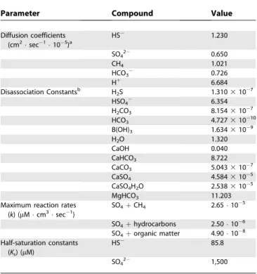
For sediments encompassed by the rhizosphere, sulfide, sulfate, methane, DOC, and hydrogen ion concentration profiles were determined iteratively prior to model implementation using a central difference scheme:
Ciðtþ1Þ¼CiþDðCiþ12CiþCi1Þ k Ci KsþCi
ð11Þ
whereCi(t)is concentration in cell i at time t, D is the diffusion
coefficient, k is the maximum reaction rate, and Ks is the half-saturation constant for the reaction (Table 2). Reactions included anaerobic methane oxidation (equation 17), tubeworm sulfide uptake rate (equation 8), and carbonate precipitation rate (equation 22). The concentration in each 232 cm cell was calculated at 1 h time steps. At the end of each year, diffusion distance increased. The number of cells (total diffusion distance) was determined by the average root length ofL. luymesipopulations as realized in independent runs of the population growth model described above, and included here as model input only. A separate function was fitted to each of the concentration profiles:
Ci¼ ðC0C‘ÞeadþC‘ ð12Þ
wheredis radial distance. The relationship between the parametera and distance was used to generate concentration profiles for each disc comprising the rhizosphere. Because of the tight linear relationship between diffusion distance and the shape of the curve, concentration profiles could be generated for a disc of any size using the following function:
ahs¼adb ð13Þ
whereais 1.7344 andbis 1.0104 for HS,ais 0.2111 andbis 0.3363 for SO42, andais 0.1626 andbis 0.2518 for CH4. Diffusional fluxes of sulfide, sulfate, and methane were calculated according to the first and second derivatives of the concentration profiles as determined by the diameter of each disc.
Model implementation.The model estimates sulfide availability to the aggregation as a whole by summing the fluxes separately determined for each 2-cm disc composing the rhizosphere. Depth-dependant boundary conditions were set for each disc separately based on the sediment profiles (Figure 5). Diffusional fluxes into each disc were calculated from the shape of the concentration profiles according to the following function [48]:
dC dt¼
1 r
d dr rDs
dC dr
ð14Þ
whereC is concentration, r is disc radius, and Ds is the diffusion coefficient corrected for porosity by:
Ds¼
Do
1þnð1/Þ ð15Þ
whereDois the diffusion coefficient corrected for temperature and pressure,nis the chemical species-specific constant, and/is porosity. The value ofnwas set to 2.75 as this was found to be a reasonable fit for all chemical species examined [49]. The ionic states of each species at the average pH value of tubeworm-dominated sediments (7.78) were used for the determination of diffusion coefficients. Porosity was determined from the following function:
/z¼ ð/0/‘Þeazþ/‘ ð16Þ
Figure 5.Concentration Profiles of Sulfate, Sulfide, and DOC
Points represent average concentration at a given depth from 13 sediment cores taken around the periphery of tubeworm aggrega-tions (see Materials and Methods and original data in [13,28]). Best-fitted line based on least squares fit of equation 9.
where/zis porosity at depthz,/0is porosity at the sediment–water interface, and/‘is porosity at infinite depth; /0was set at 0.841,/‘
at 0.765, andaat 0.210, as determined from the best fit with the porosity data (Figure 6) from Morse et al. [28].
Diffusion across the sediment–water interface of the rhizosphere was also considered as an additional input of sulfate and hydrogen ions. This was included as one-dimensional diffusion across a circular surface (subtracting the area encompassed by the tubeworm tubes) with diffusion distance equal to rhizosphere diameter, and concen-tration differential from seawater concenconcen-tration to the average concentration within the rhizosphere. Sulfate and hydrogen ion diffusion across the root surface was then added (if included in the set of model realizations) as simple Fickian diffusion. Concentration differential was the difference between internal concentration and average concentration for each disc of the rhizosphere assuming roots were evenly proportioned according to the volume encom-passed by each disc. Internal sulfate concentration and pH (Table 2) represented an average of the values determined forR. pachyptila[22], a hydrothermal vent tubeworm. Internal sulfate concentrations and pH ofL. luymesihave not been reported, but these values are generally consistent within taxa [50]. Uptake of sulfide and release of sulfate were summed across the entire tubeworm population, again assuming an even distribution of roots within the rhizosphere. The paucity of empirical data on the location of any individual tubeworm’s roots within an aggregation precluded modeling space explicitly; therefore, it is assumed that each individual has equal access to the resources available within the rhizosphere.
Within the rhizosphere, sulfide generation may be limited by sulfate supply, electron donor availability, or sulfate reduction rate. Sulfate supply was determined as the sum of flux across the series of discs approximating the rhizosphere dome, across the sediment– water interface, and from root sulfate (if available). Available sulfate is utilized for anaerobic methane oxidation first (the more energeti-cally favorable process), then hydrocarbon and organic matter degradation. Electron donors included methane, complex hydro-carbons, and buried organic material. Solid and liquid phase hydrocarbons and organic material were assumed to be homogenous within the rhizosphere. Methane supply was determined as the sum of
flux across each rhizosphere disc boundary. Hydrocarbon and organic material concentrations were determined as the amounts encompassed within the rhizosphere volume minus that oxidized in previous years. Sulfate reduction rate was determined from the relative amounts of the various electron donors with higher rates (0.71lmolml1h1) for methane oxidation and lower rates (0.083
lmol ml1 h1) for organic matter or hydrocarbon degradation [39]. Microbes carrying out these processes are assumed to be evenly distributed within the rhizosphere.
Total hydrogen sulfide availability to the aggregation was determined as the sum of sulfide diffusion and advection across each rhizosphere disc and sulfide generated within the rhizosphere from sulfate reduction according to the following reactions:
SO24 þCH4!HSþHCO3 þH2O ð17Þ
SO2
4 þ2CH2O!HSþ2HCO3 þH2O ð18Þ
SO24 þ1:47CnH2nþ2!HS
þ
1:47HCO
3 þH2O ð19Þ Bicarbonate (HCO3) is generated at a 1:1 stoichiometry during anaerobic methane oxidation and a 2:1 stoichiometry in the degradation of organic material. As hydrocarbons are degraded forming smaller chain hydrocarbons and organic acids, bicarbonate is generated at different stoichiometries. Because different-sized hydrocarbons and organic acids were not accounted for in the model, a rough average of these stoichiometries (1.47:1) based on toluene, ethylbenzene, xylene, and hexadecane degradation [18] was used to determine the amount of bicarbonate generated per mole of carbon. Hydrogen ions are also used up in a 1:1 stoichiometry with sulfate in the sulfate reduction half reaction as included in reaction 17.
In order to account for carbonate precipitation, the model traced DIC concentration, calcium concentration, hydrogen ion concen-tration, buffer capacity, carbonate saturation, and carbonate precip-itation rate. The buffer state of the rhizosphere was calculated to determine changes in pH resulting from hydrogen ion flux. Buffer capacity (b) was calculated using the following function [51]:
b¼2:3 ½H
þ þ ½OH þ ½A½B
½A þ ½B
1
þ:::þ
½A½B ½A þ ½B
n
ð20Þ
whereAandBrepresent the concentrations of the various acids and bases in the buffer system. In addition to hydrogen and hydroxyl ions, the buffer system included carbonate (CO2, H2CO3, HCO3, and CO32), sulfide (H2S and HS), sulfate (HSO4and SO42), and borate (B[OH]4and B[OH]3) speciation. Current pH was used to determine the ionic state of each species according to temperature-, pressure-, and salinity-corrected disassociation constants when available [51,52] (Table 2). Change in pH was determined from hydrogen ion flux and buffer capacity as follows:
Table 2.
Parameters Involved in Diagenetic Model
Parameter Compound Value
Diffusion coefficients (cm2sec1105)a
HS 1.230
SO42 0.650
CH4 1.021
HCO3 0.726
Hþ 6.684
Disassociation Constantsb H
2S 1.3103107
HSO4 6.354
H2CO3 8.1543107
HCO3 4.72731010
B(OH)3 1.6343109
H2O 1.320
CaOH 0.040
CaHCO3 8.722
CaCO3 5.0433107
CaSO4 4.5843105
CaSO4H2O 2.5383105
MgHCO3 11.203
Maximum reaction rates (k) (lMcm3sec1)
SO4þCH4 2.65105
SO4þhydrocarbons 2.50106 SO4þorganic matter 4.90108 Half-saturation constants
(Ks) (lM)
HS 85.8
SO42 1,500
aDiffusion coefficients all corrected for temperature, pressure, and salinity according to Stumm and Morgan [51] and
Pilson [52].
bAll disassociation constants corrected for temperature, salinity, and pressure according to Stumm and Morgan [51]
and Pilson [52] except: CaOH, no correction; CaHCO3, CaSO4, CaSO4H2O, MgHCO3, temperature only; H2CO3, temperature and salinity only; and HSO4, temperature and pressure only.
DOI: 10.1371/journal.pbio.0030077.t002
Figure 6.Sediment Porosity Values
Points represent average porosity at a given depth from 13 sediment cores taken around the periphery of tubeworm aggregations (see Materials and Methods and original data in [13,28]). Best-fitted line based on least squares fit of equation 9.
dpH dt ¼
d½Hþ dt
b ð21Þ
Saturation state is highly dependent on the degree to which calcium and bicarbonate form complexes with other ions. The‘‘free’’calcium was determined as the proportion of calcium that is not associated with complexed bicarbonate (HCO3), carbonate (CO32), hydroxyl (OH), or sulfate (SO42) ions. Free carbonate was determined as the amount not forming complexes with calcium (Caþ) or magnesium
(Mgþ) ions in solution. Saturation state was then calculated from the product of the concentrations of free calcium and carbonate divided by the solubility product constant. If the saturation state was above one, then carbonate precipitation occurred at a rate determined by:
d½CaCO3 dt ¼k1½Ca
þ½HCO
3 þk3½Caþ½CO3 ð22Þ
wherek1is 0.00597 lmol1sec1andk3= 0.456 lmol1sec1[51]. Because there is no empirical relationship between weight percent of carbonate and sediment porosity in tubeworm-dominated sediments [28], precipitation did not directly affect porosity. Precipitation was accounted for in the model by subtracting the volume of carbonate precipitate from the total volume encompassed by the rhizosphere.
At the end of each annual time step, model output included average length of individuals, population size, sulfide uptake rate, sulfide supply rate, root sulfate flux (if included), root hydrogen ion
flux, amount of sulfide supply accounted for by each process (sulfide seepage, anaerobic methane oxidation, organic matter degradation, and hydrocarbon degradation), number of individuals that could be supported by sulfide supply, carbonate precipitation rate, volume of carbonate precipitate, and pH.
Acknowledgments
We would like to acknowledge K. Montooth, P. Hudson, and five anonymous reviewers for providing helpful comments on drafts of the manuscript. We are indebted to J. Freytag, S. Dattagupta, D. Bergquist, R. Carney, and R. Sassen for the many discussions and advice provided. EEC acknowledges funding from the Center for Environmental Chemistry and Geochemistry at Pennsylvania State University and the Nancy Foster Scholarship Program at the National Oceanographic and Atmospheric Administration (NOAA). This work was supported by the U.S. Minerals Management Service, the NOAA National Undersea Research Program, and the National Science Foundation.
Competing interests.The authors have declared that no competing interests exist.
Author contributions.EEC, MAA, and CRF conceived and designed the experiments. EEC performed the experiments and analyzed the data. KS and RSA contributed reagents/materials/analysis tools. EEC,
MAA, KS, and CRF wrote the paper. &
References
1. van der Heijden MGA, Klironomos JN, Ursic M, Moutoglis P, Streitwolf-Engel R, et al. (1998) Mycorrhizal fungal diversity determines plant biodiversity, ecosystem variability and productivity. Nature 396: 69–72. 2. Stachowicz JJ, Hay ME (1999) Mutualism and coral persistence: The role of
herbivore resistance to algal chemical defense. Ecology 80: 2085–2101. 3. Treude T, Boetius A, Knittel K, Wallmann K, Jørgensen BB (2003)
Anaerobic oxidation of methane above gas hydrates at hydrate ridge, NE Pacific Ocean. Mar Ecol Prog Ser 264: 1–14.
4. Luff R, Wallmann K, Aloisi G (2004) Numerical modelling of carbonate crust formation at cold vent sites: Significance for fluid and methane budgets and chemosynthetic biological communities. Earth Planet Sci Lett 221: 337–353. 5. Wallman K, Linke P, Suess E, Bohrmann G, Sahling H, et al. (1997) Quantifying fluid flow, solute mixing, and biogeochemical turnover at cold vents of the eastern Aleutian subduction zone. Geochim Cosmochim Acta 61: 5209–5219.
6. Childress JJ, Fisher CR (1992) The biology of hydrothermal vent animals: Physiology, biochemistry, and autotrophic symbioses. Oceanogr Mar Biol Annu Rev 30: 337–441.
7. Julian D, Gaill F, Wood E, Arp AJ, Fisher CR (1999) Roots as a site of hydrogen sulphide uptake in the hydrocarbon seep vestimentiferan Lamellibrachiasp. J Exp Biol 202: 2245–2257.
8. Freytag JK, Girguis PR, Bergquist DC, Andras JP, Childress JJ, et al. (2001) A paradox resolved: Sulphide acquisition by roots of seep tubeworms sustains net chemoautotrophy. Proc Nat Acad Sci U S A 98: 13408–13413. 9. Bergquist DC, Andras JP, McNelis T, Howlett S, van Horn MJ, et al. (2003)
Succession in Gulf of Mexico cold seep communities: The importance of spatial variability. PSZNI Mar Ecol 24: 31–44.
10. Carney RS (1994) Consideration of the oasis analogy for chemosynthetic communities at Gulf of Mexico hydrocarbon vents. Geo-Mar Lett 14: 149– 159.
11. Bergquist DC, Ward T, Cordes EE, McNelis T, Howlett S, et al. (2003) Community structure of vestimentiferan-generated habitat islands from upper Louisiana slope cold seeps. J Exp Mar Biol Ecol 289: 197–222. 12. Cordes EE, Bergquist DC, Shea K, Fisher CR (2003) Hydrogen sulphide
demand of long-lived vestimentiferan tube worm aggregations modifies the chemical environment at hydrocarbon seeps. Ecol Lett 6: 212–219. 13. Arvidson RS, Morse JW, Joye SB (2004) The sulfur biogeochemistry of
chemosynthetic cold seep communities, Gulf of Mexico, USA. Mar Chem 87: 97–119.
14. Joye SB, Boetius A, Orcutt BN, Montoya JP, Schulz HN, et al. (2004) The anaerobic oxidation of methane and sulfate reduction in sediments from Gulf of Mexico cold seeps. Chem Geol 205: 219–238.
15. Hoehler TM, Alperin MJ, Albert DB, Martens CS (1994) Field and laboratory studies of methane oxidation in an anoxic marine sediment; evidence for a methanogen-sulfate reducers consortium. Global Biogeo-chem Cycles 8: 451–463.
16. Boetius A, Ravenschlag K, Schubert CJ, Rickert D, Widdel F, et al. (2000) A marine microbial consortium apparently mediating anaerobic oxidation of methane. Nature 407: 623–626.
17. Thiel V, Peckmann J, Richnow HH, Luth U, Reitner J, et al. (2001) Molecular signals for anaerobic methane oxidation in Black Sea seep carbonates and a microbial mat. Mar Chem 73: 97–112.
18. Zwolinski MD, Harris RF, Hickey WJ (2000) Microbial consortia involved in the anaerobic degradation of hydrocarbons. Biodegradation 11: 141–158. 19. Formolo MJ, Lyons TW, Zhang C, Kelley C, Sassen R, et al. (2004)
Quantifying carbon sources in the formation of authigenic carbonates at gas hydrate sites in the Gulf of Mexico. Chem Geo 205: 253–264. 20. Brooks JM, Kennicutt MC, Fisher CR, Macko SA, Cole K, et al. (1987)
Deep-sea hydrocarbon seep communities: Evidence for energy and nutritional carbon sources. Science 238: 1138–1142.
21. MacAvoy SE, Macko SA, Joye SB (2002) Fatty acid carbon isotope signatures in chemosynthetic mussels and tube worms from Gulf of Mexico hydro-carbon seep communities. Chem Geol 185: 1–8.
22. Goffredi SK, Childress JJ, Lallier FH, Desauliniers NT (1999) The ionic composition of the hydrothermal vent tubewormRiftia pachyptila:Evidence for the elimination of SO42and Hþand for a CL/HCO3shift. Physiol
Biochem Zool 72: 296–306.
23. Bergquist DC, Urcuyo IA, Fisher CR (2002) Establishment and persistence of seep vestimentiferan aggregations from the upper Louisiana slope of the Gulf of Mexico. Mar Ecol Prog Ser 241: 89–98.
24. MacDonald IR, Buthman DB, Sager WW, Peccini MB, Guinasso NL (2000) Pulsed oil discharge from a mud volcano. Geology 28: 907–910. 25. MacDonald IR, Guinasso NL, Ackleson SG, Amos JF, Duckworth R, et al.
(1993) Natural oil slicks in the Gulf of Mexico are visible from space. J Geophys Res 98: 16351–16364.
26. Bergquist DC, Williams FM, Fisher CR (2000) Longevity record for deep-sea invertebrate. Nature 403: 499–500.
27. Sassen R, Joye S, Sweet ST, DeFritas DA, Milkov AV, et al. (1999) Thermogenic gas hydrates and hydrocarbon gases in complex chemo-synthetic communities, Gulf of Mexico continental slope. Org Geochem 30: 485–497.
28. Morse JW, Arvidson RS, Joye S (2002) Inorganic biogeochemistry of cold seep sediments In: MacDonald IR, editor. Stability and change in chemo-synthetic communities, northern Gulf of Mexico. Report for U.S. Depart-ment of Interior, Minerals ManageDepart-ment Service, Contract #1435–01-96-CT-30813. pp. 9.1–9.93.
29. Lin S, Morse JW (1991) Sulfate reduction and iron sulfide mineral formation in Gulf of Mexico anoxic sediments. Am J Sci 291: 55–89. 30. Tyler PA, Young CM (1999) Reproduction and dispersal at vents and cold
seeps. J Mar Biol Assoc U K 79: 193–208.
31. Gardiner SL, Jones ML (1985) Ultrastructure of spermiogenesis in the vestimentiferan tube wormRiftia pachyptila(Pogonophora: Obturata). Trans Am Microsc Soc 104: 19–44.
32. Young CM, Va´zquez E, Metaxas A, Tyler PA (1996) Embryology of vestimentiferan tube worms from deep-sea methane/sulphide seeps. Nature 381: 514–516.
33. Nelson K, Fisher CR (2000) Absence of cospeciation in deep-sea vestimentiferan tube worms and their bacterial endosymbionts. Symbiosis 28: 1–15.
34. McMullin ER, Hourdez S, Schaeffer SW, Fisher CR (2003) Phylogeny and biogeography of deep sea vestimentiferan tubeworms and their bacterial symbionts. Symbiosis 34: 1–41.
Comparative degradation rates of chitinous exoskeletons from deep-sea environments. Mar Biol 143: 405–412.
37. Pruski AM, Fiala-Me´dioni A, Fisher CR, Colomines JC (2000) Composition of free amino acids and related compounds in invertebrates with symbiotic bacteria at hydrocarbon seeps in the Gulf of Mexico. Mar Biol 136: 411– 420.
38. Girguis PR, Childress JJ, Freytag JK, Klose K, Stuber R (2002) Effects of metabolite uptake on proton-equivalent elimination by two species of deep-sea vestimentiferan tubeworm,Riftia pachyptilaandLamellibrachiacf luymesi:Proton elimination is a necessary adaptation to sulfide-oxidizing chemoautotrophic symbionts. J Exp Biol 205: 3055–3066.
39. Aharon P, Fu B (2000) Microbial sulfate reduction rates and oxygen isotope fractionations at oil and gas seeps in deepwater Gulf of Mexico. Geochim Cosmochim Acta 62: 233–246.
40. Aharon P, Fu B (2003) Sulfur and Oxygen isotopes of coeval sulfate-sulfide in pore fluids of cold seep sediments with sharp redox gradients. Chem Geol 195: 201–218.
41. Kennicutt MC 2nd, McDonald TJ, Comet PA, Denoux GJ, Brooks JM (1992) The origins of petroleum in the northern Gulf of Mexico. Geochim Cosmochim Acta 56: 1259–1280.
42. Sassen R, MacDonald IR, Requejo AG, Guinasso NL, Kennicutt MC 2nd, et al. (1994) Organic geochemistry of sediments from chemosynthetic communities, Gulf of Mexico slope. Geo-Mar Lett 14: 110–119.
43. Saunders JA, Thomas RC (1996) Origin of ‘exotic’ minerals in Mississippi salt dome cap rocks: Results of reaction-path modeling. Appl Geochem 11: 667–676.
44. Mana Capelli S, Busalmen JP, de Sanchez SR (2001) Hydrocarbon bioremediation of a mineral-base contaminated waste from crude oil extraction by indigenous bacteria. Int Biodeterior Biodegradation 47: 233– 238.
45. Delille D, Delille B, Pelletier E (2002) Effectiveness of bioremediation of crude oil contaminated subantarctic intertidal sediment: The microbial response. Microb Ecol 44: 118–126.
46. Mills MA, Bonner JS, McDonald TJ, Page CA, Autenrieth RL (2003) Intrinsic bioremediation of a petroleum-impacted wetland. Mar Pollut Bull 46: 887– 899.
47. Kennicutt MC, Brooks JM, Bidigare RR, Denoux GJ (1988) Gulf of Mexico hydrocarbon seep communities. I. Regional distribution of hydrocarbon seepage and associated fauna. Deep-Sea Res 35: 1639–1651.
48. Boudreau BP (1997) Diagenetic models and their implementation. New York: Springer-Verlag. 417 p.
49. Iversen N, Jorgensen BB (1993) Diffusion coefficients of sulphate and methane in marine sediments: Influence of porosity. Geochim Cosmochim Acta 57: 571–587.
50. Schmidt-Nielsen K (1997) Animal physiology: Adaptation and environ-ment, 5th ed. Cambridge: Cambridge University Press. 607 p.
51. Stumm W, Morgan JJ (2000) Aquatic chemistry. New York: John Wiley and Sons. 1,022 p.
52. Pilson MEQ (1998) An introduction to the chemistry of the sea. Upper Saddle River (New Jersey): Prentice Hall. 431 p.
53. MacDonald IR, Boland GS, Baker JS, Brooks JM, Kennicutt MC 2nd, et al. (1989) Gulf of Mexico hydrocarbon seep communities. II. Spatial distribution of seep organisms and hydrocarbons at Bush Hill. Mar Biol 101: 235–247.
54. Rudinicki MD, Elderfield H, Mottl MJ (2001) Pore fluid advection and reaction in sediments of the eastern flank, Juan de Fuca Ridge, 488N. Earth Planet Sci Lett 187: 173–189.
55. Carson B, Holmes ML, Umstattd K, Strasser JC, Johnson HP (1991) Fluid expulsion from the Cascadia accretionary prism: Evidence from porosity distribution direct measurements, and GLORIA imagery. Philos Trans R Soc Lond A Math Phys Sci 335: 331–340.
56. Henry P, Lallemant S, Nakamura K, Tsunogai U, Mazzotti S, et al. (2002) Surface expression of fluid venting at the toe of the Nankai wedge and implications for flow paths. Mar Geol 187: 119–143.
57. Olu K, Lance S, Sibuet M, Henry P, Fiala-Medioni A, et al. (1997) Cold seep communities as indicators of fluid expression patterns through mud volcanoes seaward of the Barbados accretionary prism. Deep-Sea Res 44: 811–841.
58. Levin LA, Ziebis W, Mendoza GF, Growney VA, Tryon MD, et al. (2003) Spatial heterogeneity of macrofauna at northern California methane seeps: Influence of sulfide concentration and fluid flow. Mar Ecol Prog Ser 256: 123–139.
59. Wiedicke M, Sahling H, Delisle G, Faber E, Neben S, et al. (2002) Characteristics of an active vent in the fore-arc basin of the Sundra Arc, Indonesia. Mar Geol 184: 121–141.