Annales
Geophysicae
Modelling of the ring current in Saturn’s magnetosphere
G. Giampieri and M. K. Dougherty
Space and Atmospheric Physics, Imperial College, London, UK
Received: 16 April 2003 – Revised: 24 June 2003 – Accepted: 27 June 2003 – Published: 1 January 2004
Abstract. The existence of a ring current inside Saturn’s magnetosphere was first suggested by Smith et al. (1980) and Ness et al. (1981, 1982), in order to explain various fea-tures in the magnetic field observations from the Pioneer 11 and Voyager 1 and 2 spacecraft. Connerney et al. (1983) formalized the equatorial current model, based on previous modelling work of Jupiter’s current sheet and estimated its parameters from the two Voyager data sets. Here, we inves-tigate the model further, by reconsidering the data from the two Voyager spacecraft, as well as including the Pioneer 11 flyby data set.
First, we obtain, in closed form, an analytic expression for the magnetic field produced by the ring current. We then fit the model to the external field, that is the difference between the observed field and the internal magnetic field, consider-ing all the available data. In general, through our global fit we obtain more accurate parameters, compared to previous models. We point out differences between the model’s pa-rameters for the three flybys, and also investigate possible deviations from the axial and planar symmetries assumed in the model. We conclude that an accurate modelling of the Saturnian disk current will require taking into account both of the temporal variations related to the condition of the mag-netosphere, as well as non-axisymmetric contributions due to local time effects.
Key words. Magnetospheric physics (current systems; plan-etary magnetospheres; plasma sheet)
1 Introduction
First observations of Saturn’s magnetic field were made by the Pioneer 11 spacecraft in 1979. These observations re-vealed the existence of an internal magnetic field with a sur-prisingly small dipole tilt (< 1 degree) and with a high de-gree of axisymmetry (Smith et al., 1980; Acu˜na and Ness, 1980). Perturbations in the magnetic field due to current Correspondence to:G. Giampieri
sheet crossings were also observed. The flybys by the Voy-ager 1 (1980) and VoyVoy-ager 2 (1981) spacecraft confirmed the surprising nature of the internal field, but also revealed the need to include the effect of external sources of current (Acu˜na et al., 1981). Studies of Voyager 1 magnetic field observations in the middle magnetosphere led Connerney et al. (1981b) to conclude that the planet is surrounded by a eastward flowing ring current in the equatorial plane. This conclusion was confirmed by the subsequent Voyager 2 ob-servations (Connerney et al., 1983).
Models of the magnetic field initially utilised Pioneer 11 and Voyager 1 and 2 data separately (see, e.g. Connerney et al., 1982; Acu˜na et al., 1983; Connerney et al., 1984; Davis and Smith, 1986), but eventually all three data sets were com-bined (Davis and Smith, 1990; Connerney, 1993). These data provide a clear indication that Saturn, contrary to other mag-netized planets, has a planetary field almost exactly axisym-metric with respect to the spin axis.
The nature of the unusual internal planetary field at Saturn will be revisited by the Cassini spacecraft during Saturn Orbit Insertion in July 2004, when the spacecraft will pass remark-ably close to the planet (0.3Rsabove the surface), as well as
during numerous close approaches to the planet during the 4-year orbital tour (see Dougherty et al., 2003). The possi-bility of combining measurements taken along many orbits, as opposed to a single flyby, will allow for an unprecedented accuracy in the determination of the internal field.
The plan of the paper is as follows. First, we obtain an ana-lytical expression for the magnetic field produced by the ring current model first proposed by Connerney et al. (1981a). We then perform a least-squares fit on all available flyby data, including those from Pioneer 11. Finally, we consider the in-bound and outin-bound passes separately, in order to highlight local time asymmetries in the ring current.
2 The ring current model
µ0I0
∞
R
0
J0(ρx)J0(ax)sinh(Dx)e−|z|x dxx |z|> D
Bρ(z, ρ, a)=
µ0I0
∞
R
0
J1(ρx)J0(ax)sinh(zx)e−Dx dxx |z| ≤D
sign(z)µ0I0
∞
R
0
J1(ρx)J0(ax)sinh(Dx)e−|z|x dxx |z|> D, (2)
whereJn(x)is the Bessel function of ordern. In the
right-hand-side of Eqs. (1)–(2) we have made explicit the depen-dence ona, the inner edge of the disk. Thus, if we now require the disk’s outer edge to be finite at, sayr = b, we simply need to subtract from Eq. (1) the same expressions withbin place ofa, i.e.Bz(finite disk)=Bz(a)−Bz(b), and
similarly forBρ. Note that the azimuthal componentBφis
identically null because of the axial symmetry of the model, and in the following we will neglect it altogether. Note also thatI0has the units1of Current×Length−1, so that the to-tal current in the disk is given byI = 2I0Dlog(b/a). By replacing in Eq. (1) the Bessel functions with argumentρx, with their power series expansion, and integrating term by term, we eventually find
Bz(z, ρ, a)=
µ0I0 2
(
log
(z+D+ξ
a)
(z−D+ηa)
+
∞
X
k=1
(−1)k(2k−1)!ρ2k
22k(k!)2
Po
2k−1[(z−D)/ηa]
η2k a
−P o
2k−1[(z+D)/ξa]
ξ2k a
)
(3)
Bρ(z, ρ, a)=µ0I0
X
k=0
(−1)k(2k)!ρ2k+1
22k+2k!(k+1)!
Po
2k[(z−D)/ηa]
η2ak+1
−P o
2k[(z+D)/ξa]
ξa2k+1
, (4)
where
ξa≡
p
(z+D)2+a2, η
a≡
p
(z−D)2+a2,
and thePnm(x)are the associated Legendre polynomials. 1Note that Eqs. (10)–(12) in Connerney et al. (1981a) are
dimen-sionally incorrect. However, their Eqs.(13)-(15) and subsequent ones are correct (see Edwards et al., 2001)
η2k ρ
−
ξ2k ρ
(5)
Bρ(z, ρ, a)=
µ0I0 2ρ
(
2sign(z)min(|z|, D)+
ηρ−ξρ−
∞
X
k=1
(−1)k(2k−2)!a2kρ
22k(k!)2
"
P21k−1[(z−D)/ηρ]
η2k ρ
−P
1
2k−1[(z+D)/ξρ]
ξ2k ρ
# )
, (6)
where now
ξρ ≡
q
(z+D)2+ρ2, η
ρ ≡
q
(z−D)2+ρ2.
We stress that Eqs. (3)–(4) are exactly equivalent to Eqs. (5)–(6). The choice of which ones to use is purely a matter of convenience: in practice, since one takes only a few terms in the infinite sums, it is necessary, in order to as-sure fast convergence to the exact value, to use Eq. (2) when
ρ < a, and Eq. (3) whenρ > a. For example, it is easy
to show that the approximate expressions for the field com-ponents given in Edwards et al. (2001) can be obtained from Eqs. (2)–(3) by truncating the sums overkatkmax=1. How-ever, as pointed out in Bunce and Cowley (2003), those ap-proximations, originally obtained for the Jovian disk, are less useful in Saturn’s analysis, especially near the edges of the disk. With our analytical formulas (2)–(3), it is now straight-forward to extend the approximations to any desired order. In particular, we have found that, by increasingkmaxfrom 1 to 6, the average error in the field modelling components de-creases from a few nT to less than 0.1 nT. This accuracy is sufficient, since, as we will see in the next section, the resid-uals rms average is of the order of a few nT. This ensures that the errors in the estimated parameters are solely due to noise in the data and the inadeguacy of the model (e.g. the axisym-metric assumption, or the 1/ρ dependency), rather than in-accuracies in the formula for the field model. Moreover, the advantage of an analytical formula is obvious, since no nu-merical integration is necessary, in order to obtain the field’s components.
3 Results of the fit
−20 −15 −10 −5 0 5 10 15 20 −20
−10 0 10 20
∆
Bz
(nT)
Voyager 1
−20 −15 −10 −5 0 5 10 15 20 −20
−10 0 10 20
∆
Bρ
(nT)
time from CA (hrs)
ρ = 17 12 6.4 3.4 6.7 12 16
Fig. 1.Voyager 1 external field and models. The upper panel shows the1Bzcomponent, the lower one the1Bρcomponent, both expressed
in nT. The horizontal axis is time (in hours) from closest approach, which occurred at 23:73 spacecraft even time (SCET). The equatorial distanceρ(inRs) is shown in the bottom panel. The solid line is the field of the model ring current. The dotted line corresponds to model A.
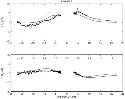
−25 −20 −15 −10 −5 0 5 10 15 20 25 −20
−10 0 10 20
∆
Bz
(nT)
Voyager 2
−25 −20 −15 −10 −5 0 5 10 15 20 25 −20
−10 0 10 20
∆
Bρ
(nT)
time from CA (hrs)
ρ = 17 13 9.4 5.3 3.5 5.3 8.9 12 16
Fig. 2.Voyager 2 data and models (same as Fig. 1). SCET at closest approach is 03:35.
around Saturn. The first step consists of eliminating the contribution from sources inside the planet. For the inter-nal field, we have considered both the Z3 model by Con-nerney et al. (1982), based on the two Voyager spacecraft data only, and theSPV model by Davis and Smith (1990), based on an extensive analysis of all the flyby data combined together. These two models vary only in the values of the dipole, quadrupole and octupole moments. By repeating our analysis with both theZ3 andSPV models, we are able to
conclude that differences in the internal parameters between the two models do not significantly affect the values of the disk parameters, although theSPV model produces slightly smallest residuals.2 Since we are not including the internal field parameters in our fit, we have discarded data collected within the inner 4Rs of Saturn’s magnetosphere. Also, data
2This may be simply due to the fact that we do not apply any
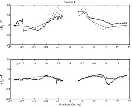
−25 −20 −15 −10 −5 0 5 10 15 20 25 −20
−10 0 10 20
∆
Bρ
(nT)
time from CA (hrs)
ρ = 17 14 10 5.8 4 5.7 9.9 14 17
Fig. 3.Pioneer 11 data and models. The dotted and dashed lines correspond to model A and B, respectively. Note the inbound magnetopause
crossing att = −20 h. The large disturbance inBρ at aroundt =15 h can be associated with a periodicity in the magnetic field near the rotation period. This has been postulated as due to the existence of a low latitude magnetic anomaly (Espinosa and Dougherty, 2000). At closest approach, SCET = 16:45.
−20 −15 −10 −5 0 5 10 15 20 −20
−10 0 10 20
∆
Bz
(nT)
Voyager 1
−20 −15 −10 −5 0 5 10 15 20 −20
−10 0 10 20
∆
Bρ
(nT)
time from CA (hrs)
ρ = 17 12 6.4 3.4 6.7 12 16
Fig. 4.Same as Fig. 1, with inbound and outbound observations analyzed separately. Note how the outer edge of the disk becomes closer to
the planet during the inbound pass (refer also to Table 1).
outside 20Rs were removed before the fit, in order to
mini-mize the effects of magnetopause currents (Saturn’s dayside magnetospheric radius being of the order of 16–20Rs). No
other external contributions, besides those due to the disk, have been considered in this analysis.
Figures 1–3 show, for each of the three flybys, the exter-nal1Bzand1Bρcomponents of the magnetic field (i.e. the
−25 −20 −15 −10 −5 0 5 10 15 20 25 −20
−10 0 10 20
∆
Bz
(nT)
Voyager 2
−25 −20 −15 −10 −5 0 5 10 15 20 25 −20
−10 0 10 20
∆
Bρ
(nT)
time from CA (hrs)
ρ = 17 13 9.4 5.3 3.5 5.3 8.9 12 16
Fig. 5. Same as Fig. 2, with inbound and outbound observations analyzed separately. The outbound model is now a much better fit to the
observations, implying a thicker and more extended disk on the dawn side of the planet (see Table 1).
by Bunce and Cowley (2003) for that particular flyby (‘model B’). The cusps in the model lines indicate when the space-craft entered or left the ring current region. These crossings do not occur in the Voyager 2 case (Fig. 2), due to the high inclination of the Voyager 2 trajectory. We have obtained the geometrical parameters of the disk, i.e. a,b,D, and the current parameterµ0I0, for each of the three orbits, through a large-scale least-squares fit algorithm, using the reflective Newton method. The values of the parameters are given in Table 1, along with the analogous quantities from models A and B. The last column in Table 1 shows the rms average of the fit residuals, which provides a measure of the quality of the fit.
4 Discussion
From Table 1, we can conclude that our global least-squares fit, using the more accurate disk model allows, in general, for a significant improvement in our knowledge of the model’s parameters, compared to previous models, which were not optimal in a least-squares sense.
In general, however, it appears that a single current disk model does not fit both the inbound (dayside) and outbound (dawn flank) observations equally well. We believe that this asymmetry reflects both a dependence on local time and on the state of the magnetospheric cavity, which is not compat-ible with the assumption of an axisymmetric disk. Similar anisotropies were also observed in the charged particles den-sity distributions. Previous studies of Saturn’s total magnetic field have already confirmed the need to use a different set of external terms for inbound and outbound orbits (see, e.g. Davis and Smith, 1986). Accordingly, we have considered
Table 1. Disk model’s parameters: inner radius a, outer radius
b, half-thicknessD, and current parameterµ0I0. The first 2 rows shows the parameters’ values for Model A (Connerney et al., 1983) and B (Bunce and Cowley, 2003), respectively. The last column gives the rms average of the residuals. Numbers in parentheses are the residuals rms averages obtained with Model A or B, respec-tively, from the Voyager and Pioneer data. Units used areRs for lengths, and nT for field magnitudes
a b D µ0I0 rms
Model A 8.0 15.5 3.0 60.4
Model B 6.5 12.5 2.0 76.5
Voyager 1 7.9 16.4 2.6 54.4 2.5 (2.8)
Voyager 2 7.2 13.7 2.1 56.8 2.9 (4.2)
Pioneer 11 6.4 13.9 1.8 50.8 3.9 (4.6)
Voyager 1 IN 7.6 15.3 3.1 40.0 1.5 (3.0)
Voyager 2 IN 6.1 12.0 1.5 52.3 2.2 (5.7)
Pioneer 11 IN 6.8 12.2 1.9 51.1 2.9 (4.1) Voyager 1 OUT 8.0 18.0 2.4 62.0 2.0 (2.7) Voyager 2 OUT 8.2 18.0 2.5 60.0 0.9 (1.4) Pioneer 11 OUT 6.4 18.0 2.8 40.0 3.6 (5.1)
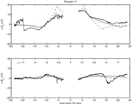
−25 −20 −15 −10 −5 0 5 10 15 20 25 −20
−10 0 10 20
∆
Bρ
(nT)
time from CA (hrs)
ρ = 17 14 10 5.8 4 5.7 9.9 14 17
Fig. 6.Same as Fig. 3, with inbound and outbound observations analyzed separately. As for the Voyager 1 case, the disk during the inbound
pass appears to be more compressed than during the outbound.
for example, from Table 1 we can see that the outbound tra-jectory usually requires a larger value ofbcompared to the inbound data, as would be expected for an extended magne-tospheric cavity on the dawn versus dayside sector.
The results shown in Table 1 clearly reveal the need for a nonaxially symmetric current sheet model at Saturn, where a range of differing best fit current sheet parameters result dur-ing both inbound and outbound passes for the same space-craft flyby. These parameters do seem, however, to be con-sistent between one flyby period and the next, for similar magnetospheric conditions. For example, both Pioneer 11 and Voyager 2 inbound flybys observed the magnetosphere in a contracted state, and the current parameterµ0I0, which results for these two flybys, is very similar. In addition, the values derived for both the inner and outer edge of the cur-rent disk, as well as its thickness, are comparable. This is in contrast to the parameters derived for the Voyager 1 inbound flyby, when the magnetosphere was in an intermediate state, where a lower current parameter, an extended current sheet extent and a greater current sheet thickness result (revealing a possible correlation between the current sheet thickness and radial extension).
The Voyager 1 and 2 outbound flybys saw the magneto-sphere in a steadily inflating state (with Voyager 2, in par-ticular, being greatly inflated, possibly as a result of being immersed in the Jovian magnetotail at the time). This re-sulted in current sheet parameters of both flybys being very similar in comparison to the Pioneer 11 values for a rather compressed but expanding magnetosphere.
The sources of plasma at Saturn are still not well under-stood, in contrast to the case of Jupiter, where the dominance of the Io plasma source is very clear. Hence, there is no Io-type mechanism which can clearly be identified inside
Sat-urn’s magnetosphere as being the main source of plasma. In fact, a variety of sources is assumed to contribute to the ions, which, in turn, generate the disk current. These source include the planet’s ionosphere, the rings, the icy satellites, neutral H clouds, and Titan. Note that all of these sources are located at various radial distances from the planet, rang-ing from very close to the planet, out to the boundary of the magnetosphere. Hence, in order to be able to better model the Saturnian ring current, not only will magnetometer data from the Cassini orbiter be necessary, but a better understanding of the various plasma sources and sinks within the magneto-sphere will be required.
Acknowledgements. We thank Emma Bunce, Stephane Espinosa,
and Paul Henderson for helpful discussions.
Topical Editor T. Pulkkinen thanks two referees for their helping in evaluating this paper.
References
Acu˜na, M. H. and Ness, N. F.: The Magnetic Field of Saturn: Pio-neer 11 Observations, Science, 207, 444–446, 1980.
Acu˜na, M. H., Connerney, J. E. P., and Ness, N. F.: Topology of Saturn’s Main Magnetic Field, Nature, 292, 721–726, 1981. Acu˜na, M. H., Connerney, J. E. P., and Ness, N. F.: TheZ3Zonal
Harmonic Model of Saturn’s Magnetic Field: Analyses and Im-plications, J. Geophys. Res., 88, 8771–8778, 1983.
Bunce, E. and Cowley, S. W. H.: A Note on the Ring Current in Sat-urn’s Magnetosphere: Comparison of Magnetic Data Obtained During the Pioneer 11 and Voyager 1 and 2 Flybys, Ann. Geo-physicae, 21, 661–669, 2003.
Connerney, J. E. P., Acu˜na, M. H., and Ness, N. F.: Saturn’s ring current and inner magnetosphere, Nature, 292, 724–726, 1981b. Connerney, J. E. P., Ness, N. F., and Acu˜na, M. H.: Zonal harmonic model of Saturn’s magnetic field from Voyager 1 and 2 observa-tions, Nature, 298, 44–46, 1982.
Connerney, J. E. P., Acu˜na, M. H., and Ness, N. F.: Currents in Saturn’s Magnetosphere, J. Geophys. Res., 88, 8779–8789, 1983. Connerney, J. E. P., Davis, Jr., L., and Chenette, D. L.: Magnetic Field Models, in: Saturn, edited by Gehrels, T. and Matthews, M. S., University of Arizona Press, pp. 354–377, 1984. Connerney, J. E. P.: Magnetic Fields of the Outer Planets, J.
Geo-phys. Res., 98, 18 659–18 679, 1993.
Davis, Jr., L. and Smith, E. J.: New Models of Saturn’s Magnetic Field Using Pioneer 11 Vector Helium Magnetometer Data, J. Geophys. Res., 91, 1373–1380, 1986.
Davis, Jr., L. and Smith, E. J.: A Model of Saturn’s Magnetic Field Based on All Available Data, J. Geophys. Res., 95, 15 257– 15 261, 1990.
Dougherty, M. K., Kelloch, S., Southwood, D. J., Balogh, A., et al.: The Cassini Magnetic Field Investigations, Space Sci. Rev.,
2003, in press.
Edwards, T. M., Bunce, E. J., and Cowley, S. W. H.: A Note on the Vector Potential of Connerney et al.’s Model of the Equatorial Current Sheet in Jupiter’s Magnetosphere, Planet. Space Sci., 49, 1115–1123, 2001.
Espinosa, S. A. and Dougherty, M. K.: Periodic perturbations in Saturn’s magnetic field, Geophys. Res. Lett., 27, 2785, 2000. Ness, N. F., Acu˜na, M. H., Lepping, R. P., Connerney, J. E. P.,
Behannon, K. W., and Burlaga, L. F.: Magnetic Field Studies by Voyager 1: Preliminary Results at Saturn, Science, 212, 211– 217, 1981.
Ness, N. F., Acu˜na, M. H., Behannon, K. W., Burlaga, L. F., Con-nerney, J. E. P., and Lepping, R. P.: Magnetic Field Studies by Voyager 2: Preliminary Results at Saturn, Science, 215, 558– 563, 1982.