Local structure of the magnetotail current sheet: 2001 Cluster
observations
A. Runov1, V. A. Sergeev2, R. Nakamura1, W. Baumjohann1, S. Apatenkov2, Y. Asano1, T. Takada1, M. Volwerk1,3, Z. V¨or¨os1, T. L. Zhang1, J.-A. Sauvaud4, H. R`eme4, and A. Balogh5
1Space Research Institute, Austrian Academy of Sciences, A-8042 Graz, Austria 2St. Petersburg University, St. Petersburg, Russia
3MPE, Garching, Germany 4CESR/CNRS, Toulouse, France 5IC, London, UK
Received: 11 August 2005 – Revised: 8 November 2005 – Accepted: 15 November 2005 – Published: 7 March 2006
Abstract. Thirty rapid crossings of the magnetotail current sheet by the Cluster spacecraft during July–October 2001 at a geocentric distance of 19REare examined in detail to ad-dress the structure of the current sheet. We use four-point magnetic field measurements to estimate electric current den-sity; the current sheet spatial scale is estimated by integra-tion of the translaintegra-tion velocity calculated from the magnetic field temporal and spatial derivatives. The local normal-related coordinate system for each case is defined by the combining Minimum Variance Analysis (MVA) and the cur-lometer technique. Numerical parameters characterizing the plasma sheet conditions for these crossings are provided to facilitate future comparisons with theoretical models. Three types of current sheet distributions are distinguished: center-peaked (type I), bifurcated (type II) and asymmetric (type III) sheets. Comparison to plasma parameter distributions show that practically all cases display non-Harris-type behavior, i.e. interior current peaks are embedded into a thicker plasma sheet. The asymmetric sheets with an off-equatorial cur-rent density peak most likely have a transient nature. The ion contribution to the electric current rarely agrees with the current computed using the curlometer technique, indicating that either the electron contribution to the current is strong and variable, or the current density is spatially or temporally structured.
Keywords. Magnetospheric physics (Magnetotail, Plasma sheet)
1 Introduction
Current sheet structure is an important property of plasma boundaries, which determines their stability against pertur-bations and explosive disruptions. This characteristic is, Correspondence to:A. Runov
however, very difficult to measure in space; so in previous years the theory was mostly based on a signal, simple, 1-D solution, known as Harris sheet (after Harris, 1962). Its basic property is that both current and plasma density vary across the sheet as cosh−2(z/L), whereas the sheet is considered to be isothermal (withTe=Ti) and with equal contributions from protons and electrons to the electric current. In the last century, the overwhelming majority of theoretical analysis was done using the Harris-type sheet models. At the same time the information about the different structure of real tail current sheets was slowly accumulated.
Flapping motion of the magnetotail current sheet mani-fests itself as both large-amplitude (a few tens of nT) and short duration (tens of seconds to several minutes), often re-peating variations of the magnetic field main component, ob-served by spacecraft in the plasma sheet. Being an interest-ing phenomenon itself, the flappinterest-ing provides a tool to probe the internal structure of the current sheet. A number of past studies addressed the problem of current sheet internal struc-ture based on observations from single or dual (ISEE-1/2) spacecraft, and different techniques have been suggested to characterize the current sheet scale and structure. Fairfield et al. (1981) tried the ion gyroradius technique and inter-preted a set of very rapid (with durations of 10–60 s) neu-tral sheet crossings by the IMP-8 spacecraft at X= –32RE as a wave propagating in the sunward-anti-sunward direc-tion. They estimated the current sheet flapping velocity to be 100–300 km/s and the apparent current sheet thickness to beh∼1000–2000 km.
andVn is the normal velocity of the current sheet, calcu-lated as a function of time. The profiles of the electric cur-rent density versus distance from the sheet center (where Bl=0) showed a very thick sheet (h≤10000 km) with low cur-rent density (j∼4 nA/m2) for the first crossing, a much thin-ner and more intensive (h∼2500 km andj∼15 nA/m2) sheet with a slightly asymmetric maximum and “shoulders” of a weaker current density for the second case, and an extremely strong (j∼50 nA/m2) current sheet with a half-thickness of 3000 km for the third case. The structures were not uniform and show embedded layers with scales of 1000 km.
Sergeev et al. (1993) analyzed 10 neutral sheet cross-ings by the ISEE 1/2 spacecraft (estimated separation about 470 km across the current sheet) atX∼–11REduring a sub-storm. Considering theBxdifference between the two space-craft (as a measure of current density) against the averageBx (as measure of the position in the sheet), different types of current sheet distributions were found. They included cur-rent peaks embedded in the sheet center (during the substorm growth phase), a distinct example of a thin bifurcated current sheet during fast plasma flow (presumably near the recon-nection site), as well as examples of turbulent and transient-dominated distributions. The estimated current sheet half-thicknesshvaried between 650 km (∼2 gyroradii of 10 keV proton in the lobe field, detected prior to the current disrup-tion) and∼4000 km or∼12 external gyroradii.
Using another method, fitting ISEE 1/2 magnetic field data to the Harris function, Sanny et al. (1994) inferred that the current sheet thickness at X∼–13REvaried from severalRE at the beginning of the substorm growth phase toh∼0.1RE just after expansion onset. They also suggested a multi-point calculation approach, based on calculations of the convective derivative, which allows one to reconstruct an effective ver-tical scale of the current sheet during its crossing by a group of spacecraft.
An alternative technique to estimate the thickness of a flap-ping current sheet using ion bulk velocity measurements has been suggested in Sergeev et al. (1998). If the up/down mo-tions of the current sheet are seen as positive/negative vari-ations of the bulk velocityZ-component, the current sheet scalehcan be estimated from the linear regression slope be-tweenVZ and∂tBx. For a set of current sheet crossings by the AMPTE/IRM spacecraft atR∼12–18RE, they found the sheet scales varying from∼2 to 0.2RE and electric current densities from 4 to 30 nA/m2.
Analyzing theBx-occurrence frequency distribution dur-ing multiple current sheet crossdur-ings (expected to be inversely proportional to dBx/dz gradients in the case of vertical flapping motions), measured by the Geotail spacecraft at ∼100REin the tail, Hoshino et al. (1996) found distributions consistent with a double-peaked (bifurcated) current density profile. Because such structures were observed during fast ion flows, Hoshino et al. (1996) attributed them to slow shock structures downstream of a reconnection site. Later, Asano et al. (2003), using electron and ion moments from Geotail to calculate the electric current density, inferred similar double-peak structures at a distance of 15REdowntail. They argued
that such structures appear as a local or/and temporal en-hancement of the current density away from the neutral sheet, associated with current sheet thinning and flapping prior to substorm onset. In that case the current sheet bifurcation may not be associated with magnetic reconnection.
Greatly enhanced possibilities of measuring spatial gra-dients have appeared after the launch of the four-spacecraft Cluster system, whose early results showed a number of ex-amples of complex behavior and structure of the tail cur-rent sheet. The fast dynamics of the curcur-rent sheet struc-ture was demonstrated by Nakamura et al. (2002), provid-ing the example of rapid change from the Harris type to the bifurcated shape during a fast earthward flow event, and by Runov et al. (2005b), who documented the opposite change during substorm expansion. Distinct examples of stable (dur-ing 10–15 min intervals) bifurcated distributions dur(dur-ing sub-storm times have been provided by Runov et al. (2003b) and Sergeev et al. (2003). The need for careful determination of a proper coordinate system follows from statistical studies by Sergeev et al. (2004) and Runov et al. (2005a), who showed that flapping current sheets are unusually strongly tilted in theY–Z plane. Moreover, Asano et al. (2005) and Runov et al. (2005a) found that off-center peak distributions of the current density seem to be a frequent property of the current sheet.
As seen from this Introduction, the rapidly growing evi-dence of different possible current distributions requires one to perform a systematic study of the current sheet structure using all Cluster possibilities, to infer the current density dis-tribution in the proper coordinate system. This will be the purpose of our paper, in which, as a continuation of the pre-vious publication (Runov et al., 2005a), we investigate the profiles of the current density and ion moments during care-fully selected rapid crossings of the current sheet. We focus on the current structure and also provide the lists of quanti-tative current sheet characteristics, which may be useful for further comparison with theoretical models.
The 1-s averaged magnetic field data from the Cluster Flux Gate Magnetometer (FGM, Balogh et al., 2001) and 2-spin (normal mode) or 1-spin (burst mode) averaged data from the Cluster Ion Spectrometry experiment (CIS, R`eme et al., 2001) are used in the analysis presented in this paper.
2 Selection of events and local coordinate system
Table 1.Selected events.
N datea t0b(UT) IMFyc IMFzc AEd Ye,RE Nif, cm−3 Vxf Vyf Vzf, km/s Tif, keV PO/PHg BLh, nT
1 0724 17:18:53 –8.2 0.9 439 –13.0 0.66 25 –15 27 6.0 0.05 36.8 2 0724 17:44:55 –7.0 1.5 428 –13.0 0.62 47 3 –28 6.0 0.07 35.3 3 0727 10:39:17 –0.6 0.4 169 –11.0 0.29 –38 –2 –75 8.1 0.04 26.1 4 0803 09:17:34 –8.4 –3.3 213 –9.7 0.60 93 2 –117 8.0 0.05 39.8 5 0812 15:28:06 –7.5 –6.8 166 –7.3 1.77 17 16 –33 2.1 0.05 37.9 6 0812 15:29:45 –7.5 –6.8 166 –7.3 1.71 2 16 52 2.3 0.04 37.6 7 0822 08:57:41 –0.6 2.4 118 –4.6 0.39 75 –10 49 6.4 0.05 27.4 8 0910 08:03:32 1.0 –0.5 69 0.8 0.69 10 –10 –25 1.5 0.04 21.0 9 0910 08:12:15 1.1 –0.5 59 0.8 0.73 0 –19 –28 1.2 0.03 20.2 10 0912 14:19:03 6.7 –2.5 288 1.7 0.40 14 –12 –8 4.6 0.14 25.7 11 0912 14:22:45 6.7 –1.8 292 1.6 0.42 112 –4 7 5.1 0.16 26.6 12 0914 22:55:00 –4.9 –4.6 119 2.0 2.30 37 –57 0 1.0 0.08 32.6 13 0914 23:10:03 –3.5 –8.8 193 2.0 2.43 –28 –63 –66 1.1 0.09 33.4 14 0914 23:50:06 –5.0 –4.3 250 2.1 3.17 17 –32 –28 1.4 0.12 42.6 15 0924 08:04:20 –4.3 5.6 23 5.0 0.87 0 –32 –45 2.6 0.42 30.1 16 0924 08:07:58 –5.3 4.5 22 5.0 0.86 29 –26 –10 2.4 0.43 30.0 17 0926 22:26:27 –0.7 0.3 139 5.9 1.09 –22 34 –25 2.1 0.19 27.5 18 0926 22:27:24 –0.7 0.3 140 5.9 1.15 –3 5 –63 2.0 0.17 28.3 19 1001 09:42:45 10.0 –1.1 625 6.8 0.24 17 –17 5 4.8 0.49 31.9 20 1001 09:50:06 9.9 –0.5 627 6.8 0.13 538 –277 –260 4.1 7.21 20.7 21 1008 12:30:43 6.3 2.5 286 8.4 0.57 –28 18 –4 6.8 0.20 36.2 22 1008 12:49:16 6.9 1.6 326 8.5 0.44 22 –43 –12 4.3 0.25 32.9 23 1008 13:00:21 7.2 0.6 366 8.5 0.36 59 –47 –8 5.5 0.44 33.0 24 1008 13:06:50 7.4 1.2 400 8.5 0.16 10 –19 –39 7.0 0.48 26.2 25 1013 08:07:39 –4.6 –1.2 227 9.7 0.33 172 –19 –18 6.9 0.19 25.9 26 1020 09:28:21 5.5 –2.1 208 11.0 0.69 71 –29 –25 4.5 0.27 32.5 27 1020 09:38:05 3.9 –2.5 238 11.0 0.60 10 7 –33 3.5 0.32 32.0 28 1020 09:46:55 3.1 –4.1 240 11.0 0.61 11 45 3 3.2 0.38 28.4 29 1020 09:57:12 2.9 –4.7 234 11.1 0.57 4 13 –14 3.1 0.39 26.8 30 1020 09:58:57 3.1 –4.8 232 11.1 0.63 –6 –16 1 3.2 0.34 25.9
a) date format: mmdd of 2001; b) the instance of|Bx bc|=min(|Bx bc|);
c) 16-min averaged IMFy- andz-components from ACE spacecraft at the shiftedt0; d) 2-h averagedAEatt0from the Kyoto monitor;
e) theYAGSMcoordinate of the Cluster barycenter att0;
f) the average ion density, components of the bulk velocity and temperature during the crossing (Cluster 1 and 4 CODIF data within
|Bx|≤0.5BL);
g) the average O+and H+pressures ratio during the crossing (Cluster 1 and 4 CODIF data within|Bx| ≤0.5BL);
h) the asymptotic magnetic field value in the lobe, estimated from pressure balance:BL=(B2+2µ0Pi)1/2,Pi =PH++PO+), the electron
pressure is not included.
selected 78 events of the neutral sheet crossing, according to these selection criteria.
To make an investigation of the current sheet structure pos-sible, we visually analyzed the calculated magnetic field gra-dient∇Bl(wherelis the maximum variance eigenvector re-sulting from the MVA applied for the magnetic field time series at the Cluster barycenter), to find cases with smooth, monotonous profiles of∇Bl versusBl, for which the struc-ture may be defined. Comparing∇nBl, where∇nis the com-ponent of the gradient along the local normal to the current sheet (see the definition below), and|∇Bl|profiles, we se-lected cases with a minimum change inf the current sheet orientation during flapping (when both curves do not deviate
much from each other). Finally, we have chosen 30 profiles (which is a compromise number to be representative enough and possible to visualize) which were most suitable for the spatial profile reconstruction crossings covering large por-tions of the current sheet on both the northern and southern halves, for further analysis.
Table 1 presents the dates and UT of the selected crossings, the 16-min average values of IMFY- andZ-components (in nT) from the ACE spacecraft around time shifted t0;
Table 2.Local normal coordinate systema.
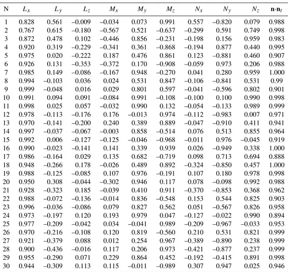
N Lx Ly Lz Mx My Mz Nx Ny Nz n·nt
1 0.828 0.561 –0.009 –0.034 0.073 0.991 0.557 –0.820 0.079 0.988 2 0.767 0.615 –0.180 –0.567 0.521 –0.637 –0.299 0.591 0.749 0.998 3 0.872 0.478 0.102 –0.446 0.856 –0.231 –0.198 0.156 0.959 0.983 4 0.920 0.319 –0.229 –0.341 0.361 –0.868 –0.194 0.877 0.440 0.995 5 0.975 0.020 –0.222 0.187 0.476 0.861 0.123 –0.881 0.460 0.907 6 0.926 0.131 –0.353 –0.372 0.170 –0.908 –0.059 0.973 0.206 0.988 7 0.985 0.149 –0.086 –0.167 0.948 –0.270 0.041 0.280 0.959 1.000 8 0.994 –0.103 0.036 0.024 0.531 0.847 –0.106 –0.841 0.531 0.99 9 0.999 –0.048 0.016 0.029 0.801 0.597 –0.041 –0.596 0.802 0.901 10 0.991 0.094 0.091 –0.084 0.991 –0.108 –0.100 0.100 0.990 0.998 11 0.998 0.025 0.057 –0.032 0.990 0.132 –0.054 –0.133 0.989 0.999 12 0.978 –0.113 –0.176 0.176 –0.013 0.974 –0.112 –0.983 0.007 0.971 13 0.970 –0.141 –0.200 0.240 0.389 0.889 –0.047 –0.910 0.411 0.941 14 0.997 –0.037 –0.067 –0.003 0.858 –0.514 0.076 0.513 0.855 0.964 15 0.992 0.006 –0.127 –0.125 –0.046 –0.968 –0.011 0.976 –0.045 0.919 16 0.990 –0.023 –0.141 0.141 0.339 0.939 0.026 –0.949 0.338 1.000 17 0.986 –0.164 0.029 0.135 0.682 –0.719 0.098 0.713 0.694 0.888 18 0.948 –0.266 0.178 –0.026 0.489 0.892 –0.324 –0.850 0.457 1.000 19 0.988 –0.125 –0.085 0.107 0.976 –0.191 0.107 0.180 0.978 0.998 20 0.950 0.308 –0.044 –0.302 0.946 0.117 0.078 –0.098 0.992 0.988 21 0.928 –0.323 0.185 –0.039 0.410 0.911 –0.370 –0.853 0.368 0.962 22 0.988 –0.072 –0.136 –0.014 0.836 –0.548 0.153 0.544 0.825 0.903 23 0.996 –0.036 –0.086 0.079 0.827 0.562 0.051 –0.567 0.826 0.958 24 0.973 –0.197 0.120 0.193 0.979 0.047 –0.127 –0.022 0.990 0.894 25 0.977 –0.209 –0.042 0.034 –0.041 0.989 –0.209 –0.967 –0.033 0.953 26 0.970 –0.216 –0.108 0.120 0.819 –0.560 0.210 0.531 0.821 0.999 27 0.921 –0.379 0.088 0.012 0.254 0.967 –0.389 –0.890 0.238 0.999 28 0.900 –0.436 –0.016 0.117 0.206 0.973 –0.421 –0.877 0.237 0.999 29 0.955 –0.290 0.071 0.229 0.864 0.452 –0.192 –0.415 0.891 0.998 30 0.944 –0.309 0.113 0.115 –0.011 –0.989 0.307 0.947 0.025 0.946
a)GSMcomponents of local normal coordinate system with the quality check (see explanations in the text).
Vx,y,z(H+only), the ratio of proton andO+ions pressures and average lobe magnetic fieldBL=(B2+2µ0Pi)1/2. The density, temperature, velocity and pressure are averaged over Bx≤0.5BLsamples using Cluster 1 and 4 CODIF data.
For each selected crossing the local normal coordinate sys-tem l,m,n was defined. As usual, the l axis is directed along the maximum variance eigenvector (from MVA, ap-plied to the magnetic field at the barycenter, Bbc). The m-axis is aligned along the component of the electric cur-rentj=µ−01∇×Bperpendicular tol, averaged over the neu-tral sheet (|Bx|<5 nT):m=l×[j/j×l]. Finally, then-axis is directed perpendicular tolandm: n=l×m. Components of the local orthogonal coordinate systeml,m,nare given in Table 2. In 13 cases of of 30, the tilt angle of the nor-malφ=atan(|ny|/|nz|)was larger than 60◦(the normalnis directed mainly alongYGSM), in 9 cases 30◦<φ<60◦, and only in 8 casesφ<30◦(the normal has a nominal orientation alongZGSM ).
To check the quality of the local coordinate system, we compared the normalnwith the normal vectornt, resulting from multi-point timing analysis (Harvey, 1998). The scalar
products of two normalsn·nt are also presented in Table 2. The angle between these two normals varies between 0 and 27◦, with a median value 8.9◦, confirming that the normals
are very accurately defined in our set of current sheet cross-ings.
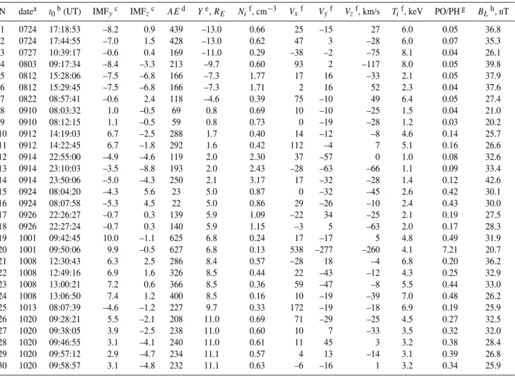
Figure 1 surveys the time series ofl,m,nmagnetic field components at the Cluster barycenter,Bbc=0.25P4α=1Bα, where α is a spacecraft number. The crossing duration τ varies from 35 s to 300 s with the 144-s median. In 12 cases the average normal component of the magnetic field in the sheet center (where|Bl|<5 nT) is very small:Bn<1 nT, and only in three cases is the mean value is large, about 5 nT. The most frequent value is 1.3 nT. The current-aligned com-ponent of magnetic fieldBm is typically larger (in the sheet center) thanBn, it varies in the wide range 0 to 0.3BL and its median value isBmis 3.5 nT.
3 Current sheet structures
cur-τ,
s
Bl (black), Bm (red), Bn (blue), nT
1
2
3
4
5
6
7
8
9
10
11
12
13
14
15
16
17
18
19
20
21
22
23
24
25
26
27
28
29
30
Fig. 1. Time series of the magnetic field at the Cluster barycenter in local normal coordinate system{l, m,n}(see text for details) for
rent densityj=µ−01∇×B, calculated using a linear curl esti-mator technique, based on the tetrahedron reciprocal vectors method (Chanteur, 1998).
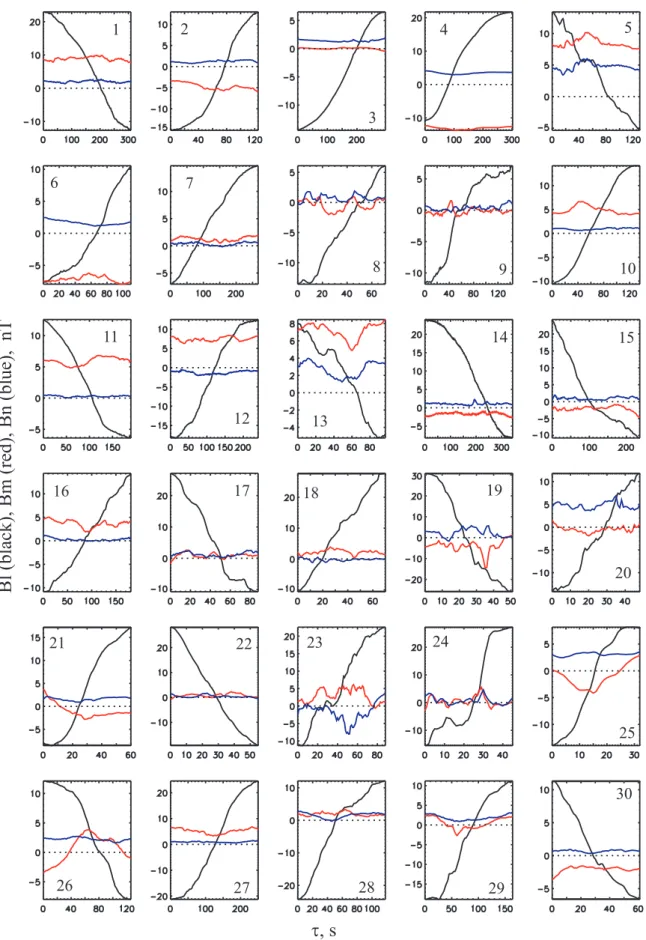
Figure 2 presents profiles of the absolute value of the current density (red curves) and the perpendicular cur-rentj⊥=(jm2+jn2)1/2 (blue curves) versusBl at the Cluster barycenter, normalized by the average value of the magnetic field in the lobe (BL, see Table 1). Dashed curves show the profiles of the corresponding Harris current as a function of a variableb=Bl/BLrunning between –1 and 1:
jH = BL µ0λ[
1−b2], (1)
where the Harris scaleλis defined for each crossing as the median of instantaneous values
λ= BL h∇nBli[
1−(Bl BL
)2]. (2)
To display scales of the observed structures we plot in Fig. 3 the profiles of the current density and the perpendicu-lar current versus the effective vertical coordinate
Z∗(t )=
Z t
t1
∂Bl ∂t [∇nBl]
−1dt′−Z∗(t
0) , (3)
wheret1andt2 are instances of the beginning and the end
of the crossing, respectively, andt0 is the time of the
neu-tral sheet crossing by the Cluster barycenter. (Details of the reconstruction procedure and its accuracy are discussed by Runov et al., 2005a.) For reference, as in Fig. 2, the dashed curves show the Harris current.
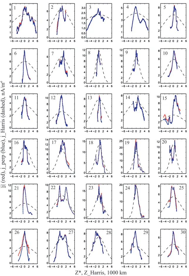
Observed current sheet structures can be subdivided into three classes: I – central sheets with single peak centered nearBl=0 (be most clear examples are # 4, 6, 10, 11, 12, 13, 21, 24, 26, 30); II – bifurcated sheets with two off-equatorial maxima of the current density and local minimum of the cur-rent density between them (#14, 20, 22, 25, 27); and III – asymmetric off-center current sheets with the current density maximum shifted from equatorial plane (#5, 7, 15, 16, 17, 18, 28, 29). Figure 4 shows a summary of the current den-sity distributions for most clear cases of these three classes, together with the average profile.
It is difficult to attribute undoubtedly cases # 1, 2, 3, 8, 9 and 23 to the described types: they have a more or less central single peak but are asymmetric or slightly bifurcated like dis-tributions of the current density as # 2. The case # 19 seems to be very peculiar. It was observed during a storm-time sub-storm on 1 October 2001 near the reconnection site (Runov et al., 2003a) in an underpopulated plasma sheet (Kistler et al., 2005) with unusual ion velocity distributions (Wilber et al., 2004). The important result is that only in two cases (19 and 24) as the current density distributed from−BL to +BLhave a profile resembling the Harris function. In both cases the current was very strong (∼25 and∼20 nA/m2, re-spectively) and the ion density was small (of 0.2 cm−3).
The average profile of the class I central sheet (Fig. 4 upper panel) is characterized by a layer between|Z∗|≤2000 km, with peak atBl∼0, where the magnetic field gradient is larger
than outside. In terms of the characteristic proton length, with a median value of 300 km, the half-thickness of the cen-tral layer is about 5–7Lcp(Lcpis the asymptotic gyroradius, calculated with the average proton temperature and the es-timated lobe magnetic field). The current density outside this layer forms the “shoulders” at about 2 nA/m2. Because the current in the class I current sheets is concentrated in the embedded layer between roughly±0.5BL, it cannot be de-scribed by the Harris function with the lobe field, calculated from the pressure balance, and used as a parameter. A more adequate fit can be done using the asymptotic magnetic field valueB0(<BL) instead ofBLin Eqs. (1) and (2). Here we used asB0the value ofBl, where the current density drops
down by a factor of 0.25 from the maximum to estimateB0.
Corresponding values of the Harris scale λ′ for the class I sheets are also given in Table 3.
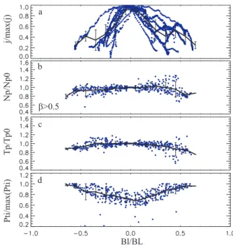
Figure 5 shows profiles of the current density (normalized by its maximum value), proton density and temperature (nor-malized by their values at the sheet center, Np0 andT p0,
Bl_bc/BL
|j| (red), j
_perp (
bl
ue), j
_Harris (dashed), nA
/m
2
1
2
3
4
5
6
7
8
9
10
11
12
13
14
15
16
17
18
19
20
21
22
23
24
25
26
27
28
29
30
Fig. 2.Hodograms of the current densityj=µ−01∇×Babsolute value (blue) and perpendicular componentj⊥=
q
jm2+jn2(red) versus main
magnetic field (Bl) for selected 30 cases. Dashed lines show the Harris function, Eq. (1), with the parameterλcalculated using an average
Z*, Z_Harris, 1000 km
|j|
(
red)
, j
_pe
rp (blue)
, j
_Harris (dashed)
, nA/m
2
1
2
3
4
5
6
7
8
9
10
11
12
13
14
15
16
17
18
19
20
21
22
23
24
25
26
27
28
29
30
Fig. 3.Profiles of absolute values of the current densitiesj(blue) andj⊥(red) versus the effective vertical coordinateZ∗, calculated from
j, nA/m
2
12
10
8
6
4
2
0
10
8
6
4
2
0
12 10 8 6 4 2 14
-6 -4 -2 0 2 4 6
Z*, 1000 km
I
II
III
Fig. 4. Averaged vertical profiles of the current density for center
peaked (class I), bifurcated (class II), and asymmetric (class III) current sheets. The Z* is calculated using Eq. (3).
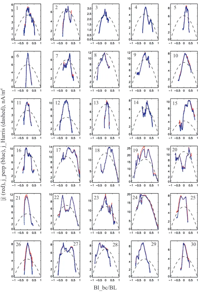
To show the class III current sheets with peaks above and below the neutral sheet on the same plot, we changed the signs ofZ∗andBl in the events with peaks below the neu-tral sheet, so that these peaks will appear atBx>0 in Fig. 7. Off-center current sheets have a scale of≤2000 km and an asymmetric profile, so that the half-thickness at the outer side is smaller (≤1500 km) than at the inner side (≥2000 km). The current density peaks were found at 0.2<Bl/BL<0.6. As in the previous cases, only samples with a correspond-ing proton-β<0.5 are used to plot the proton parameters. The density has a flat profile at Bl<0.5BL and drops at Bl/BL>0.5. The temperature profile has a broad maximum around Bl=0. The P ti has a slightly asymmetric profile with a maximum atBl∼0.5BL, a broad minimum between –0.5<Bl/BL≤0.3, and with a value atBl≤–0.5BLwhich is about 0.7 of the maximum value. Scalesh(Table 3) for the class III sheets are estimated as a half-thickness at the level ofj=0.5jmax. These estimates, as well ashfor classes I and II are very rough and are rounded off to 500 km.
Figure 8 shows an example of the asymmetric off-center current sheet. Here we present 10 min of Cluster/FGM data
Bl/BL
j/
max(j)
Np
/Np0
T
p/
T
p0
β>0.5 a
b
c
d
Pti
/max(
Pti
)
Fig. 5. Profiles of the current density(a), proton number density,
normalized by the valueN0=Np(Bl=0)(b), and proton
tempera-ture(c)normalized byT0=Tp(Bl=0), and the sum of magnetic and
ion pressures (P ti)(d), normalized by their maximum value, versus
normalized main magnetic fieldBl/BLfor class I current sheets.
on 24 September 2001, starting at 08:04:20 UT (t=0). Clus-ter crosses the neutral sheet twice (crossings 15 and 16 in Ta-ble 1). Panel (a) shows the projections of the electric current vector onto theY−Zplane and the positions of the Cluster spacecraft with respect to the barycenter. This event is sim-ilar to the one discussed by Runov et al. (2005a). Cluster observes a fold of the current sheet, traveling duskward with a velocity of∼25 km/s. The electric current at the fronts of the fold is directed almost vertically, downward at the lead-ing front (100–200 s) and upward at the second front (380– 500 s). At the leading front the current density maximum is achieved at around t=150 s, when the average magnetic field is∼15 nT. The current density decreases by a factor of 2 at the neutral sheet. Between 210 and 380 s the spacecraft stay at –10<Bx<0 nT. The current density here is three times smaller than at the leading front. At the next front the cur-rent density increases again. At this time the curcur-rent sheet seems to be slightly bifurcated. Interestingly, the kink struc-ture is associated with an enhancement of theZGSM com-ponent of the magnetic field which is current sheet aligned at the fronts, but the By GSM component, which is approx-imately normal to the fronts, remains very small (<1 nT). This example shows that the current density can change dur-ing the passage of perturbation, increasdur-ing at its fronts.
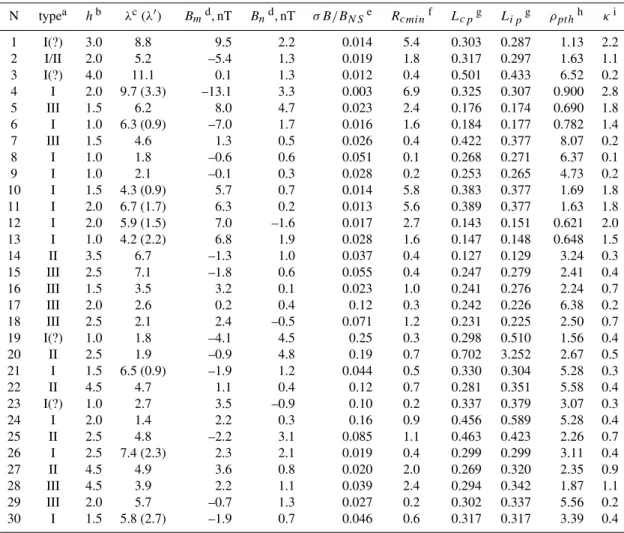
Table 3.Current sheet parameters.
N typea hb λc(λ′) Bmd, nT Bnd, nT σ B/BN Se Rcminf Lcpg Li pg ρpt hh κi
1 I(?) 3.0 8.8 9.5 2.2 0.014 5.4 0.303 0.287 1.13 2.2 2 I/II 2.0 5.2 –5.4 1.3 0.019 1.8 0.317 0.297 1.63 1.1 3 I(?) 4.0 11.1 0.1 1.3 0.012 0.4 0.501 0.433 6.52 0.2 4 I 2.0 9.7 (3.3) –13.1 3.3 0.003 6.9 0.325 0.307 0.900 2.8 5 III 1.5 6.2 8.0 4.7 0.023 2.4 0.176 0.174 0.690 1.8 6 I 1.0 6.3 (0.9) –7.0 1.7 0.016 1.6 0.184 0.177 0.782 1.4 7 III 1.5 4.6 1.3 0.5 0.026 0.4 0.422 0.377 8.07 0.2 8 I 1.0 1.8 –0.6 0.6 0.051 0.1 0.268 0.271 6.37 0.1 9 I 1.0 2.1 –0.1 0.3 0.028 0.2 0.253 0.265 4.73 0.2 10 I 1.5 4.3 (0.9) 5.7 0.7 0.014 5.8 0.383 0.377 1.69 1.8 11 I 2.0 6.7 (1.7) 6.3 0.2 0.013 5.6 0.389 0.377 1.63 1.8 12 I 2.0 5.9 (1.5) 7.0 –1.6 0.017 2.7 0.143 0.151 0.621 2.0 13 I 1.0 4.2 (2.2) 6.8 1.9 0.028 1.6 0.147 0.148 0.648 1.5 14 II 3.5 6.7 –1.3 1.0 0.037 0.4 0.127 0.129 3.24 0.3 15 III 2.5 7.1 –1.8 0.6 0.055 0.4 0.247 0.279 2.41 0.4 16 III 1.5 3.5 3.2 0.1 0.023 1.0 0.241 0.276 2.24 0.7 17 III 2.0 2.6 0.2 0.4 0.12 0.3 0.242 0.226 6.38 0.2 18 III 2.5 2.1 2.4 –0.5 0.071 1.2 0.231 0.225 2.50 0.7 19 I(?) 1.0 1.8 –4.1 4.5 0.25 0.3 0.298 0.510 1.56 0.4 20 II 2.5 1.9 –0.9 4.8 0.19 0.7 0.702 3.252 2.67 0.5 21 I 1.5 6.5 (0.9) –1.9 1.2 0.044 0.5 0.330 0.304 5.28 0.3 22 II 4.5 4.7 1.1 0.4 0.12 0.7 0.281 0.351 5.58 0.4 23 I(?) 1.0 2.7 3.5 –0.9 0.10 0.2 0.337 0.379 3.07 0.3 24 I 2.0 1.4 2.2 0.3 0.16 0.9 0.456 0.589 5.28 0.4 25 II 2.5 4.8 –2.2 3.1 0.085 1.1 0.463 0.423 2.26 0.7 26 I 2.5 7.4 (2.3) 2.3 2.1 0.019 0.4 0.299 0.299 3.11 0.4 27 II 4.5 4.9 3.6 0.8 0.020 2.0 0.269 0.320 2.35 0.9 28 III 4.5 3.9 2.2 1.1 0.039 2.4 0.294 0.342 1.87 1.1 29 III 2.0 5.7 –0.7 1.3 0.027 0.2 0.302 0.337 5.56 0.2 30 I 1.5 5.8 (2.7) –1.9 0.7 0.046 0.6 0.317 0.317 3.39 0.4
a) I- central peaked, II- bifurcated, III- asymmetric; b) half-thickness estimates, 1000 km;
c) Harris scale parameter estimates (see details in the text), 1000 km;
d) average values of current-align (Bm) and normal (Bn) components of the magnetic field in the neutral sheet (|Bl|≤5 nT);
e) the standard deviation of the magnetic field during the crossing, normalized by the average magnetic field in the neutral sheet; f) the magnetic field curvature radius minimum value, 1000 km;
g) characteristic scales: The asymptotic proton gyroradius (Lc) and the ion inertial scale (Li), 1000 km;
h) the proton thermal gyroradius in the neutral sheet, 1000 km; i) the adiabaticity parameterκ=p
Rcmin/ρp th.
(Fig. 3), parametersλ(λ′) of the corresponding Harris func-tions, Eq. (1). They are followed by current aligned (m) and normal (n) magnetic field components in the neutral sheet (|Bl|<5 nT), variability of the magnetic fieldσ B(calculated as the standard deviation within 8-s (2-spin) long intervals, normalized by the mean value of the magnetic field in the neutral sheet) and minimum magnetic field curvature radii Rcmin. The characteristic plasma scales include: asymptotic proton gyroradiusLcp[1000 km]=4.6√Ti[keV]/BL[nT]and proton inertial lengthLip[1000 km]=0.23/
p
Ni[cm−3]. We also specified values for the proton thermal gyroradiusρp th in the neutral sheet (in 1000 km) and the corresponding val-ues for the adiabaticity parameterκ=p
Rcmin/ρp th(B¨uchner
and Zelenyi, 1989). Because the minima of the magnetic field curvature radius were found within the neutral sheet in all cases, the above-writtenκ-parameter definition was used for bifurcated sheets, too (theoretically, theκ-parameter has a special definition for double-peaked current sheets; Delcourt et al., 2004).
4 Curlometer current versus proton contribution
Bl/BL
j/
max(j)
Np
/Np0
T
p/
T
p0
β>0.5 a
b
c
d
Pti
/max(
Pti
)
Fig. 6.Same as in Fig. 5 for class II current sheets.
Bl/BL
j/
max(j)
Np
/Np0
T
p/
T
p0
β>0.5 b
c a
Pti
/max(
Pti
) d
Fig. 7.Same as in Figs. 5 and 6 for class III current sheets.
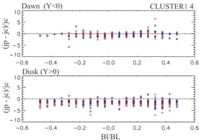
jcm andjp m as functions of the normalized main magnetic fieldBl/BLare shown in Fig. 9. It should be noted that be-cause of the current sheet tilt in theY−Zplane (see Table 2), for a majority of crossings the current aligned proton veloc-ity is contributed to by theZGSEcomponent, which is mea-sured with a significant inaccuracy, possibly resulting in the jp1andjp4differences. The velocity offset of 20 km/s with
the density 0.8 cm−3(the mean value of the density for the selected events, Table 1) givesjp∼3 nA/m2.
t, s
Bx, nT
j
,
j,
nA/m
2
a
b
e c
d
By
, nT
B
z, nT
+ +
B NS
* * *
CLUSTER 1, 2, 3, 4
|j|, jx, jy, jz
Fig. 8. Example of the class III current sheet: Cluster/FGM
data (panelsb–d), calculated current density(e)versus time (s). Panel(a)shows spacecraft separations and current vector projec-tions on theY Zplane; barycenter positions are marked by asterisks; dashed lines display the shape of the current sheet kink.
The relationship betweenjcandjpappears to be compli-cated and variable. Both proton and curlometer currents have similar profiles and values in cases 1–6 observed in the dawn sector. For the remaining cases observed mostly in the dusk sector, except for # 22 (bifurcated profile), the proton current generally has an opposite sign (negative) and can even be much larger in magnitude (cases 14, 17, 18, 23, 28). This difference does not seem to depend on the type of the current sheet structure (I, II or III).
1
2
3
4
5
6
7
8
9
10
11
12
13
14
15
16
17
18
19
20
21
22
23
24
25
26
27
28
29
30
Bl_bc/BL
j
c, jp, nA/
m , C
L
USTER
1
,
4
2
Fig. 9.Profiles of the curlometer currentm-component (black) and the corresponding proton currentjp m∼NpVmat Cluster 1 (red) and 4
We examined distributions of the electric current density, proton density, temperature and bulk velocity inside the magnetotail current sheet during 30 episodes of fast cur-rent sheet crossings by the Cluster spacecraft. Because the Cluster tetrahedron scale a during July–October 2001 was ∼1500 km, only structures with scales larger than a were studied. By showing a variety of possible distributions we also found that the observed structures can be subdivided into three groups: central current sheets (I) with a sharp maxi-mum of the current density at the neutral sheet; bifurcated current sheets (II) with two quasi-symmetric current density maxima in the northern and southern halves of the sheet and a minimum near the neutral sheet; and asymmetric off-center current sheets (III) with the current density maximum shifted away from the neutral sheet. Typical half-thicknesses of the current sheets are≤2000 km or∼5Lcpfor the classes I and III, and about 4000 km (∼10Lcp) for class II. Profiles of the class III sheets are asymmetric with respect to the current density maximum. The large variety of current density dis-tributions observed is consistent with the results by Asano et al. (2005), who used another technique (comparison ofBx components observed at two pairs of Cluster spacecraft) and a different event selection (in particular, excluding time vary-ing and strongly tilted sheets). Such a variable appearance, therefore, can be the rule for the magnetotail current sheet.
In agreement with Asano et al. (2005) we found strong de-viations from the behavior predicted by the Harris model and, in fact, the non-Harris sheets can be the rule rather than the exception, for active current sheets in the magnetotail (see also Thompson et al., 2005). For example, the center-peaked current sheet (type I) profiles, except for two cases, 19 and 24, strongly differ from the Harris function: the current den-sity is concentrated in the layer within±0.5BL, whereBL is the lobe field strength, calculated from pressure balance. Moreover, the proton density and temperature behave fairly uniform inside all types of current sheets, indicating that cur-rent density peak(s) are not simply followed by the plasma pressure variations and that they are embedded into more thicker plasma sheets.
The fact that the sum of the magnetic and ion pressures for I and II types of sheets has roughly the same values at both sides of the sheets and drops at the sheet center indicates that the total pressure is nearly conserved in these types of cur-rent sheets, and contributions from electrons (up to 15%, ac-cording to Baumjohann et al., 1989) and ions with energies exceeding 38 keV (not counted by CODIF) can be up to 30% of the aggregate H+and O+pressure in the sheet center (see also Fairfield et al., 1981). Contributions of O+ ion
pres-sure vary between 5–50% (see Table 1). The asymmetry of the proton total pressure profile in the class-III current sheets points out their transient nature.
In 16 out of the 30 studied cases the tilt angle of the cur-rent sheet normal with respect to theZGSMdirection exceeds 45◦. In 17 cases the tilt was dawnward (nY<0, nZ>0) and duskward in 13 cases (Table 2). No definite correspondence
Dusk (Y>0)
(jp
- jc
)/jc
(jp
- jc
)/jc
Bl/BL
Fig. 10. Differences of proton (jp) and curlometer (jc) currents
along themdirection in the morning(a)and evening(b)sectors, normalized by the absolute value of the curlometer current.
between IMFBy and the normal tilt was found. The tilt of the current sheet in the studied cases indicates a corrugated profile of the sheet surface, crossed by the spacecraft during flapping.
In examining AE-activity dependence (Table 1) or local plasma conditions we could not find systematic differences between events with different types or different thicknesses of the current sheets in our limited survey. (More focused efforts with a larger database are required to reveal and quan-tify the activity dependence, if it exists at all.)
Nineteen (out of 30) cases represent low velocity intervals withV <100 km/s. Two high-speed intervals (# 19 and # 20) were observed during a large substorm and show the complex structures, with most likely a single peak of current density (# 19) and with a clearly bifurcated current sheet (# 20). Ion densities and temperatures vary in a very broad range with-out any definite relation to the current sheet structures. Note that we have several examples of cold dense plasma sheets (# 5, 6, 12–14) which show structures of all three types. The relative magnetic field variability (σ Bin Table 3) was not big (generally less than 0.1) during the studied crossings, so we cannot attribute any differences in the structure of the current sheets to the effect of magnetic field fluctuations (e.g. Greco et al., 2002). The adiabaticity parameterκ is generally less than unity, which indicates non-adiabatic ion motion within the flapping current sheets. Again, no simple relation with the current sheet structure can be observed.
gyroradius) current sheet. Bifurcated profiles of the current density can also result from a trapped ion population (Zelenyi et al., 2003) and from electrostatic effects (Zelenyi et al., 2004b) and the electron pressure anisotropy (see, e.g. Ze-lenyi et al., 2004a) in thin current sheets. In a preliminary study we surveyed the proton pressure anisotropy measured by the CIS instrument, but found that usually the anisotropy is very small (deviation from isotropy less than 10%) with considerable scatter. Detailed studies of ion and electron dis-tributions in the current sheet would require a special future effort, in particular, concentrating on the data in the high-resolution instrument mode.
One source of the observed sheet variability and of non-Harris behavior could be temporal variations of the current density or the passage of localized (essentially non-1-D) cur-rent structures. In fact, the kink-perturbation, producing the flapping event in the current sheet, can carry localized asym-metric current structures. For example, in their PIC simu-lations, Karimabadi et al. (2003) have shown that the max-imum of the current density is displaced fromBx=0 during the ion-ion kink instability excitation. Sitnov et al. (2004), simulating the evolution of a bifurcated current sheet, have found quasi-rectangular kinks of the sheet with asymmet-ric off-center (and grainy) current density distributions. This could be, in particular, a reason for observing the asymmet-ric (type III) current distributions. It is difficult to explore such effects with Cluster, which, for current measurements, acts as a 1-point instrument. Some information about this could be obtained after noticing that, if the peak current is due to localized enhanced current carried by the propagating kink, the position ofjmax (say, inBl/BL coordinates) will rather be defined by the location of spacecraft rather than by theBl/BLcoordinate itself. To check this we compared the position of the peak current with the location of the mid-point of each crossing for events in classes I and III. We have found that for central sheets (class I) the peak location has no relation to the spacecraft position, whereas for asymmet-ric current events (class III) some dependence, indicating a transient nature of the asymmetric sheets, is observed. The amount of the events is, however, small, and this test should be repeated on larger statistics.
The most intriguing (and potentially most interesting) ob-servation is that, in most of cases, the proton contribution to the electric current is not the dominant contribution. The rel-ative difference between the total (curlometer-based) current and proton contribution is several times larger than the total current, indicating that it is clearly the electrons which con-tribute to the tail current in the flapping events. (The contri-bution of oxygen ions is not large,<20%, even in storm-time oxygen-dominated plasma sheets according to Kistler et al., 2005.) The possible explanation of the observed difference should take into account that the contribution of each species is a sum of its magnetic and polarization drifts (Vd), produc-ing an electric current, and electric (Vc) drifts, which does not produce the electric current (particularlyVp=Vd p+Vc for protons), Therefore, the difference between measured current density and the proton moment, shown in Fig. 10,
is(jp−jc)≃eNp(Vc−Vde)in the projection to the local
di-rection of the current vector. The electric drift contribution (Vc) can be significant (even dominant) in the presence of a large normal electric field, directed toward the neutral sheet, producing dawnward convection. This electric field along the local sheet normal, converging to the neutral sheet center and suggesting a negative electric charge in the sheet center, should be of 0.5 to several mv/m, which is comparable to the average dawn-dusk electric field (e.g. Asano et al., 2004; Wygant et al., 2005). It can also be larger in the dusk sector, where the current sheet is generally more active (e.g. Nagai et al., 1998) than in the dawn sector. A clarification of the normal electric field contribution and an explanation of the observed dawn-dusk asymmetry are challenging issues for future studies which have to incorporate the measurements of electrons available at Cluster.
Acknowledgements. We wish to thank H.-U. Eichelberger, G. Laky,
C. Mouikis, L. Kistler, E. Georgescu and E. Penou for help with data and software, M. Hoshino, L. Zelenyi, R. Treumann, A. Petrukovich, M. Sitnov, Ph. Louarn and H. Malova for fruitful dis-cussion. ACE spacecraft data are provided by N. Ness (Bartol Re-search Institute) and available on CDAWeb. We thank WDC for Ge-omagnetism, Kyoto providing AE indices. This work is supported by INTAS 03-51-3738, by RFBR N 03-02-17533 and N 03-05-20012 and by Russian Ministry of Education and Science (Intergeo-physica) grants. The work by M. Volwerk was financially supported by the German Bundesministerium f¨ur Bildung und Forschung and the Zentrum f¨ur Luft- und Raumfahrt under contracts 50 OC 0104. Topical Editor T. Pulkkinen thanks L. Zelenyi and another ref-eree for their help in evaluating this paper.
References
Angelopoulos, V., Kennel, C. F., Coroniti, F. V., Pellat, R., Kivel-son, M. G., Walker, R. J., Russell, C. T., Baumjohann, W., Feld-man, W. C., and Gosling, J. T.: Statistical characteristics of bursty bulk flow events, J. Geophys. Res., 99, 21 257–21 280, 1994.
Asano, Y., Mukai, T., Hoshino, M., Saito, Y., Hayakawa, H., and Nagai, T.: Evolution of the thin current sheet in a sub-storm observed by Geotail, J. Geophys. Res., 108, 1189, doi:10.1029/2002JA009785, 2003.
Asano, Y., Mukai, T., Hoshino, M., Saito, Y., Hayakawa, H., and Nagai, T.: Statistical study of thin current sheet evolu-tion around substorm onset, J. Geophys. Res., 109, A05 213, doi:10.1029/2004JA010413, 2004.
Asano, Y., Nakamura, R., Baumjohann, W., Runov, A., V¨or¨os, Z., Volwerk, M., Zhang, T. L., Balogh, A., Klecker, B., and R`eme, H.: How typical are atypical current sheets?, Geophys. Res. Lett., 32, L03 108, doi:10.1029/2004GL021834, 2005.
Balogh, A., Carr, C. M., Acu˜na, M. H., Dunlop, M. W., Beek, T. J., Brown, P., Fornacon, K.-H., Georgescu, E., Glassmeier, K.-H., Harris, J., Musmann, G., Oddy, T., and Schwingenschuh, K.: The Cluster magnetic field investigation: Overview of in-flight perfomance and initial results, Ann. Geophys., 19, 1207–1217, 2001,
Average plasma properties in the central plasma sheet, J. Geo-phys. Res., 94, 6597–6606, 1989.
Birn, J., Schindler, K., and Hesse, M.: Thin electron current sheets and their relation to auroral potentials, J. Geophys. Res., 109, A02 217, doi:10.1029/2003JA010303, 2004.
B¨uchner, J. and Zelenyi, L. M.: Regular and chaotic charged parti-cle motion in magnetotaillike field reversals, 1, Basic theory of trapped motion, J. Geophys. Res., 94, 11 821–11 842, 1989. Chanteur, G.: Spatial interpolation for four spacecraft: Theory,
in: Analysis Methods for Multi-Spacecraft Data, edited by: Paschmann, G. and Daly, P., ESA, Noordwijk, 349–369, 1998. Delcourt, D. C., Malova, H. V., and Zelenyi, L. M.: Dynamics of
charged particles in bifurcated current sheets: Theκ≃1 regime, J. Geophys. Res., 109, A01 222, doi:10.1029/2003JA010167, 2004.
Fairfield, D. H., Hones Jr., E. W., and Meng, C.-I.: Multiple cross-ing of a very thin plasma sheet in the Earth’s magnetotail, J. Geo-phys. Res., 86, 11 189–11 200, 1981.
Greco, A., Taktakishvili, A. L., Zimbardo, G., Veltri, P., and Zelenyi, L. M.: Ion dynamics in the near-Earth mag-netotail: Magnetic turbulence versus normal component of the average magnetic field, J. Geophys. Res., 107, 1267, doi:10.1029/2002JA009270, 2002.
Harris, E. G.: On a plasma sheet separating regions of oppositely directed magnetic field, Nuovo Cimento, 23, 115–121, 1962. Harvey, C. C.: Spatial gradients and volumetric tensor, in: Analysis
Methods for Multi-Spacecraft Data, edited by: Paschmann, G. and Daly, P., 307–322, ESA, Noordwijk, 1998.
Hoshino, M., Nishida, A., Mukai, T., Saito, Y., Yamamoto, T., and Kokubun, S.: Structure of plasma sheet in magnetotail: Double-peaked electric current sheet, J. Geophys. Res., 101, 24 775– 24 786, 1996.
Karimabadi, H., Pritchett, P. L., Daughton, W., and Krauss-Varban, D.: Ion-ion kink instability in the magnetotail: 2 Three-dimensional full particle and hybrid simulations and comparison with observations, J. Geophys. Res., 108, 1401, doi:10.1029/2003JA010109, 2003.
Kistler, L., Mouikis, C., M¨obius, E., Klecker, B., Sauvaud, J.-A., R`eme, H., Korth, A., Marocci, M. F., Lundin, R., Parks, G. K., and Balogh, A.: Contribution of nonadiabatic ions to the crosstail current and O+dominated thin current sheet, J. Geophys. Res., 110, A06 213, doi:10.1029/2004JA010653, 2005.
McComas, D. J., Russel, C. T., Elphic, R. C., and Bame, S. J.: The near-Earth cross-tail current sheet: Detailed ISEE 1 and 2 case studies, J. Geophys. Res., 91, 4287–4301, 1986.
Nagai, T., Fujimoto, M., Saito, Y., Machida, S., Terasawa, T., Naka-mura, R., Yamamoto, T., Mukai, T., Nishida, A., and Kokubun, S.: Structure and dynamics of magnetic reconnection for sub-storm onsets with Geotail observations, J. Geophys. Res., 103, 4419–4440, 1998.
Nakamura, R., Baumjohann, W., Runov, A., Volwerk, M., Zhang, T. L., Klecker, B., Bogdanova, Y., Roux, A., Balogh, A., R`eme, H., Sauvaud, J.-A., and Frey, H. U.: Fast flow dur-ing current sheet thinndur-ing, Geophys. Res. Lett., 29, 2140, doi:10.1029/2002GL016200, 2002.
R`eme, H., Aostin, C., Bosqued, J. M., Danduras, I., Lavraud, B., Sauvaud, J.-A., Barthe, A., Bouyssou, J., Camus, T., Coeur-Joly, O., et al.: First multispacecraft ion measurements in and near the Earth’s magnetosphere with the identical Cluster ion spectrome-try (CIS) experiment, Ann. Geophys., 19, 1303–1354, 2001,
SRef-ID: 1432-0576/ag/2001-19-1303.
Zhang, T. L., Volwerk, M., V¨or¨os, Z., Balogh, A., Glassmeier, K.-H., Klecker, B., R`eme, H., and Kistler, L.: Current sheet structure near magnetic X-line observed by Cluster, Geophys. Res. Lett., 30, 1579, doi:10.1029/2002GL016730, 2003a. Runov, A., Nakamura, R., Baumjohann, W., Zhang, T. L.,
Volw-erk, M., Eichelberger, H.-U., and Balogh, A.: Cluster observa-tion of a bifurcated current sheet, Geophys. Res. Lett., 30, 1036, doi:10.1029/2002GL016136, 2003b.
Runov, A., Sergeev, V. A., Baumjohann, W., Nakamura, R., Ap-atenkov, S., Asano, Y., Volwerk, M., V¨or¨os, Z., Zhang, T. L., Petrukovich, A., Balogh, A., Sauvaud, J.-A., Klecker, B., and R`eme, H.: Electric current and magnetic field geometry in flap-ping magnetotail current sheets, Ann. Geophys., 23, 1391–1403, 2005a,
SRef-ID: 1432-0576/ag/2005-23-1391.
Runov, A., Sergeev, V. A., Nakamura, R., Baumjohann, W., Zhang, T. L., Asano, Y., Volwerk, M., V¨or¨os, Z., Balogh, A., and R`eme, H.: Reconstruction of the magnetotail current sheet structure us-ing multi-point Cluster measurements, Planet. Space Sci., 53, 237–243, 2005b.
Sanny, J., McPherron, R. L., Russel, C. T., Baker, D. N., Pulkkinen, T. I., and Nishida, A.: Growth-phase thinning of the near-Earth current sheet during CDAW 6 substorm, J. Geophys. Res., 99, 5805–5816, 1994.
Sergeev, V., Angelopulous, V., Carlson, C., and Sutcliffe, P.: Cur-rent sheet measurements within a flapping plasma sheet, J. Geo-phys. Res, 103, 9177–9188, 1998.
Sergeev, V., Runov, A., Baumjohann, W., Nakamura, R., Zhang, T. L., Volwerk, M., Balogh, A., R`eme, H., Sauvaud, J.-A., Andr´e, M., and Klecker, B.: Current sheet flapping motion and structure observed by Cluster, Geophys. Res. Lett., 30, 1327, doi:10.1029/2002GL016 500, 2003.
Sergeev, V., Runov, A., Baumjohann, W., Nakamura, R., Zhang, T. L., Balogh, A., Louarn, P., Sauvaud, J.-A., and R`eme, H.: Ori-entation and propagation of current sheet oscillations, Geophys. Res. Lett., 31, L05 807, doi:10.1029/2003GL019346, 2004. Sergeev, V. A., Mitchell, D. G., Russell, C. T., and Williams,
D. J.: Structure of the tail plasma/current sheet at∼11RE and
its changes in the course of a substorm, J. Geophys. Res, 98, 17 345–17 365, 1993.
Sitnov, M. I., Guzdar, P. N., and Swisdak, M.: A model of the bifurcated current sheet, Geophys. Res. Lett., 30, 1712, doi:10.1029/2003GL017218, 2003.
Sitnov, M. I., Swisdak, M., Drake, J. F., Guzdar, P. N., and Rogers, B. N.: A model of the bifurcated current sheet: 2. Flapping motion, Geophys. Res. Lett., 31, L09 805, doi:10.1029/2004GL019473, 2004.
Thompson, S. M., Kivelson, M. G., Khurana, K. K., McPherron, R. L., Weygand, J. M., Balogh, A., R`eme, H., and Kistler, L. M.: Dynamic Harris current sheet thickness from Cluster current den-sity and plasma measurements, J. Geophys. Res., 110, A02 212, doi:10.1029/2004JA010714, 2005.
Wilber, M., Lee, E., Parks, G. K., Meziane, K., Carlson, C. W., Mc-Fadden, J. P., R`eme, H., Dandouras, I., Sauvaud, J.-A., Bosqued, J.-M., Kistler, L., M¨obius, E., McCarthy, M., Korth, A., Klecker, B., Bavassano-Cattaneo, M.-B., Lundin, R., and Lucek, E.: Cluster observations of velocity space-restricted ion distribu-tions near the plasma sheet, Geophys. Res. Lett., 31, L24 802, doi:10.1029/2004GL020265, 2004.
E. A., Balogh, A., Andre, M., Reme, H., Hesse, M., and Mouikis, C.: Cluster observations of an intense normal com-ponent of the electric field at a thin reconnecting current sheet in the tail and its role in the shock-like acceleration of the ion fluid into the separatrix region, J. Geophys. Res., 110, A09 206, doi:10.1029/2004JA010708, 2005.
Zelenyi, L. M., Malova, K. V., and Popov, V. Y.: Splitting of thin current sheets in the Earth’s magnetosphere, JETP Letters, 78, 296–299, 2003.
Zelenyi, L. M., Malova, H. V., Popov, V. Y., Delcourt, D., and Sharma, A. S.: Nonlinear equilibrium structure of thin current sheets: Influence of electron pressure anisotropy, Nonlinear Pro-cesses Geophys., 11, 579–587, 2004a.