Heterogeneous capital and consumption goods in a structurally generalized Uzawa’s model

Heterogeneous capital and consumption goods

in a structurally generalized Uzawa’s model

Wei-Bin ZHANG

Ritsumeikan Asia Pacific University, Japan wbz1@apu.ac.jp

Abstract.This paper proposes a growth model with heterogeneous capital and consumption goods and services. It structurally generalizes the Uzawa growth model by introducing heterogeneous capital and multiple consumption goods and services. We show the dynamic properties of the model and simulate the motion of the national economy with two capital goods and two services over time. We also examine effects of changes in preferences and technologies on the dynamic paths of the economy. The model with heterogeneous capital reveals different properties from those of the model with homogeneous capital. Our model shows the importance of introducing heterogeneous capital into the neoclassical growth theory. For instance, the comparative dynamic analysis shows that when the propensity to save is increased, the wealth per capita is increased initially but reduced in the long-term and the wage rate and national output level fall; the consumption levels of the two services fall even though the prices of the two services fall only slightly; the stock of the light capital good rises initially but falls in the long-term; the stock of the heavy capital good falls in association with rising in its price; the labor input of the heavy industrial sector fall and the labor inputs of the two service sectors rise while the labor input of the light industrial sector rises initially but falls in the long-term. Solow’s one-sector and Uzawa’s two-sector growth models cannot explain the structural changes with heterogeneous capital. Both Solow’s one-sector and Uzawa’s two-sector growth models show that a rise in the saving rate will increase the wealth per capita both in the short-term and in the long-term.

Keywords: heterogeneous capital goods; economic structure; growth; economic dynamics.

JEL Code: D92.

1. Introduction

necessary to treat consumption and investment differently in order to get a better understanding of business cycles.(3)

2. The two-capital and multi-service growth model

The model is based on the traditional two-sector model proposed by Uzawa (1961), although we will extend the single capital sector in the Uzawa model to the case of two capital goods and multiple services. The two capital goods sectors are called respectively the heavy and light industrial sectors. It is assumed that consumption and capital goods are different commodities. There are two capital goods sector and J consumption good (and services) sectors. Labor grows at an exogenously given exponential rate n which is assumed to be zero in this study. The assumption of zero population growth rate does not affect our analysis in the sense that we can get similar results with a positive constant growth rate (because the sectors exhibit constant returns to scale). Let subscripts h,i, and j, respectively, stand for the heavy industrial sector, the light industrial sector, and the jth’s service sector, j =1,..., J. The capital goods can be used as inputs in all the sectors in the economy. The capital goods depreciate respectively at constant exponential rates, δ_h and δ_i. A typical consumer’s utility level is dependent on the consumption goods and wealth. The industrial sectors produce the capital goods, which can be used only as production inputs. The light industrial commodity is selected to serve as numeraire. Labor and capital markets are perfectly competitive and labor force and capital are fully employed. Let N stand for the fixed labor force and w

( )

t the wage rate.

The capital good sectors

First, we describe production side of the economy. We consider that the heavy industrial sector uses heavy capital good Kh

( )

t , light industrial capital good

( )

t ,

kh and labor Nh

( )

t as inputs. We specify the heavy industrial sector’s

production function F_h

( )

t as follows

( )

( )

( )

( )

, 0 ,

,

, 1 ,

> γ β α

= γ + β + α ×

× ×

= α β γ

h h h

h h h h

h h

h

h t A K t N t k t

F h h h

(1)

where A_h is the total productivity factor. In this study, we assume A_h,α_h, β_h,

( )

( )

( ) ( )

_{( )}

( )

( ) ( )

_{( )}

( )

( ) ( )

_{( )}

, , , t k t F t p t r t N t F t p t w t K t F t p t p t r h h h h i i h h h h h h h h h h h γ = δ + β = α = δ + (2)

where p_h is the price of the heavy capital good.

The production function of the light industrial sector Fi

( )

t is a function of heavy capital good Ki

( )

t , light industrial capital good ki

( )

t , and labor Ni

( )

t as

follows

( )

( )

( )

( )

. 0 , , , 1 , > γ β α = = γ + β + α × × ×

= α β γ

i i i i i i i i i i

i t A K t N t k t

F i i i

(3)

The marginal conditions for the light industrial sector are given by

( )

( )

_{( )}

( )

,

( )

_{( )}

( )

,

( )

_{( )}

( )

. t k t F t r t N t F t w t K t F t p t r i i i i i i i i i i i h h h γ δ β α

δ = = + =

+ (4)

The service sectors

The production function of the jth’s service sector Fj

( )

t is a function of heavy capital good K_j

( )

t , light industrial capital good k_j

( )

t , and labor N_j

( )

t as follows

( )

( )

( )

( )

. , ... , 1 , 0 , , , 1 , J j t k t N t K A t F j j j j j j j j j j j j j j = > γ β α = γ + β + α × × × ×

= α β γ

(5)

The marginal conditions are

( )

( )

( )

_{( )}

( )

( )

( )

_{( )}

( )

( )

( )

_{( )}

( )

, , , t k t F t p t r t N t F t p t w t K t F t p t p t r j j j j i i j j j j j j j j h h h × × γ = δ + × × β = × × α = δ + (6)

where p_j

( )

t is the price of the jth service.

Consumer behavior

and light industrial goods at time t. Let us denote y

( )

t the current net income of the representative household. The net income consists of wage incomes and interest payment, i.e.

( )

t r

( ) ( ) ( ) ( )

t k t r t k~t w

( )

t ,

y = _h × + _i × + (7)

where k

( )

t ≡ K

( )

t /N and k~

( )

t ≡ K~

( )

t /N. We call y

( )

t the current income in the sense that it comes from consumers’ wages and current earnings from ownership of wealth. The sum of income that consumers are using for consuming, saving, or travels are not necessarily equal to the current income because consumers can sell wealth to pay, for instance, the current consumption if the current income is not sufficient for buying food and touring the country. Retired people may live not only on the interest payment but also have to spend some of their wealth. The total value of the wealth that a consumer can sell to purchase goods and to save is equal to p_h

( ) ( )

t ×k t +k~

( )

t . Here, we assume that selling and buying wealth can be conducted instantaneously without any transaction cost. The disposable income at any point of time is then equal to

( )

( )

( ) ( )

~

( )

.

ˆ t y t p t k t k t

y = + _h × + (8)

The disposable income is used for saving and consumption. The value,

( ) ( )

t k t k

( )

t ph

~

+

× in the above equation is a flow variable. Under the assumption that selling wealth can be conducted instantaneously without any transaction cost, we may consider ph

( ) ( )

t k t k

( )

t

~

+

× as the amount of the income that the

consumer obtains at time t by selling all of his wealth. Hence, at time t the consumer has the total amount of income equaling yˆ to distribute between the current consumption and future consumption (i.e., saving). In the growth literature, for instance, in the Solow model, the saving is out of the current income ,yˆ while in this study the saving is out of the disposable income which is dependent both on the current income and wealth. The implications of our approach are similar to those in the Keynesian consumption function and models based on the permanent income hypothesis, which are empirically much more valid than the approaches in the Solow model or the in Ramsey model. The approach to household behavior in our approach is discussed at length by Zhang.(8)

We assume that the utility level, U

( )

t , of a typical household is dependent

on consumption good, cj

( )

t , and savings, s

( )

t . The utility function is specified as

follows

( )

( )

( )

, ₀ , ₀ 0, 1,..., ,

1

0

0 _{t c t j J}

s t

U _j

J

j

j > =

=

∏

=

ξ λ

7

in which the parameters λ₀ and ξ_0j are, respectively, called the propensities to save and to consume services. The disposable income is allocated for consuming and saving. The budget constrain is given by

( ) ( ) ( )

ˆ

( )

.

1p t c t st y t

J

j j × j + =

∑

=

Households determine cj

( )

t and s

( )

t at each moment. Maximizing U

( )

t

subject to the budget constrain yields

( ) ( )

t c t yˆ

( ) ( )

t , st yˆ

( )

t ,

p_j × _j =ξ_j =λ (9)

where

. ,

0 1 0

0

0 1 0

0

λ ξ

λ λ

λ ξ

ξ ξ

+ ≡

+ ≡

∑

∑

= =

J

j j

J

j j

j

Let a

( )

t stand for the total wealth of the household. We have

( )

t p

( ) ( )

t k t k~

( )

t . a ≡ _h × +

According to the definition of s

( )

t the wealth accumulation is given by

( ) ( ) ( )

t st at .

a = − (10)

The equation simply states that the change in wealth is equal to the saving minus the dissaving.

Consider now an investor with one unity of money. He can either invest in heavy industrial capital goods thereby earning a profit equal to the net own-rate of return r_h(t)/p_h(t) or invest in light industrial capital goods thereby earning a profit equal to the net own-rate of return ri

( )

t . As we assume capital markets to be at competitive equilibrium at any point of time, two options must yield equal returns, i.e.

( )

( )

t r

( )

t . p

t r

i h

h = ₍₁₁₎

Assume that the labor force is always fully employed. We have

( )

( )

( )

.

1

N t N t

N t N

J

j j i

h + +

∑

=

=

(12)

( )

( )

( )

( )

,

1

t K t K t

K t K

J

j j i

h + +

∑

=

=

( )

( )

( )

~

( )

.

1

t K t k t

k t k

J

j j i

h + +

∑

=

=

(13)

The balance of demand of and supply for each consumption good is represented by

( )

t F

( )

t .

C_j = _j (14)

The change in the stock of a capital good is equal to its output minus its depreciation. We have

( )

t F

( )

t K

( )

t , K = h −δh



( )

( )

~

( )

. ~

t K t

F t

K = _i −δ_i (15)

We have thus built the model.

3. Properties of the dynamic system

This section examines properties of the dynamic system. First, we show that the motion of the economy can be expressed as three-dimensional differential equations. Before stating our analytical results, we introduce two variables

. ,

i i h

h

h r

w z

p r

w Z

δ

δ ≡ +

+ ≡

The dynamics is expressed with the two variables and the stock of capital goods 2 as the variables.

Lemma 1

The dynamics of the economy is described by the following differential equations

( )

t ₂

(

K

( ) ( ) ( )

t ,Z t , zt

)

,

K =Ψ

( ) ( ) ( )

(

, ,

)

,

1 K t Z t z t

Z =Ψ

( ) ( ) ( )

(

, ,

)

,

2 K t Z t z t

9

(A15) ⇒ w

( )

t and ri

( )

t by (A3) ⇒ ph

( )

t by (A4) ⇒ pj

( )

t , j =1,..., J, by

(A4)⇒ r_h

( )

t by (A4) ⇒ yˆ

( )

t by (A6) ⇒ Nj

( )

t , j =1,..., J, by (A10) ⇒

( )

t

K_m and k_m

( )

t , m = h,i,1,..., J, by (A.1) ⇒ F_h

( )

t by (1) ⇒ F_i

( )

t by (3)

⇒ F_j

( )

t , j =1,..., J, by (5) ⇒ c_j

( )

t and s

( )

t by (9) ⇒

( )

t

(

p

( ) ( )

t K t K~

( )

t

)

/N.

a = _h +

This lemma implies that once we solve the differential equations, then we can determine all the other variables, such as the national output, the labor distribution, capital distribution among the sectors, the rate of interests, and the wage rate.

As the expressions are tedious, it is difficult to explicitly interpret economic implications of the conditions for existence of a steady state. In the reminder of this study, we show properties of the dynamic system by simulation. We specify the parameter values for a four-sector economy as follows

, 65 . 0 ,

25 . 0 ,

6 . 0

, 2 . 0 ,

1 . 1 ,

9 . 0 ,

1 . 1 ,

1 ,

10 _{1 2}

= β =

α =

β

= α =

= =

= =

i i

h

h i

h A A A

A N

, 08 . 0 ,

04 . 0

, 75 . 0 ,

65 . 0 ,

18 . 0 ,

63 . 0 ,

23 . 0

02 10

0 2

2 1

1

= ξ =

ξ

= λ =

β =

α =

β =

α

. 06 . 0 ,

05 .

0 =

= k

h δ

δ

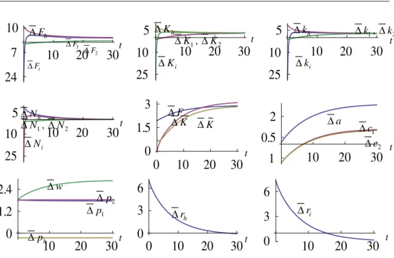
The propensity to save out of the disposable income is 86 percent, the propensity to consume service 1 is 4.6 percent, and service 2 is 9.2 percent. The total productivity factor of the light industry sector is higher than the total productivity factors of the other sectors. The depreciation rates of the heavy and light capital good are, respectively, five and six percent. As we have the differential equations from which we can determine the motion of the system, it is straightforward to plot the motion of all the variables over time. Following the computing procedure given in Lemma 1, we now simulate the model to illustrate motion of the system. The initial conditions are specified as follows

( )

0 =5, Z

( )

0 =1.5, z

( )

0 =8.1. K

We introduce the national output as

( )

t F

( )

t p

( )

t F

( )

t p1

( )

t F2

( )

t p2

( ) ( )

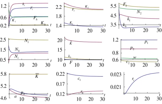
t F2 t .

As sown in Figure 1, the system does converge to a steady state. The stock of the heavy capital good changes slightly over time, while its price falls. The value of the heavy capital good falls. The value of the light capital good also falls over time. Hence, the wealth per capita falls. The prices of the two services and the wage are changed slightly over time. The consumption levels of the two services fall. The output and input levels of the heavy industrial sector falls, while the output and input levels of the light industrial sector rises. The national output level is changed slightly in association with the structural changes.

Figure 1. The motion of the economic system

Following Lemma 1, we calculate the equilibrium values of the variables as follows , 46 . 2 , 16 . 1 , 30 . 1 , 33 . 5 , 06 . 2 , 13 . 1 , 23 . 0 , 76 . 18 ~ , 67 . 4 , 86 . 9 , 63 . 0 , 92 . 0 , 19 . 1 , 84 . 5 , 137 . 0 , 023 . 0 1 2 1 2 1 = = = = = = = = = = = = = = = = N N N F F F F K K F w p p p r r i h i h h h i

10 20 30

0.2 0.6 1.2

10 20 30

1.4 1.8 2.2

10 20 30

3.5 4.5 5.5

10 20 30

0.5 1.5 2.5

0 10 20 30

10 15 20

10 20 30

0.6 0.8 1.2

10 20 30

4.6 5.2 5.8

10 20 30

0.12 0.17 0.22

10 20 30

1

. 61 . 4 , 53 . 0 ,

21 . 0 ,

01 . 10 ,

12 . 4

, 35 . 1 ,

27 . 3

, 06 . 2 ,

32 . 1 ,

66 . 0 ,

64 . 0 ,

08 . 5

2 1

2 1

2 1

2

= =

= =

=

= =

= =

= =

=

a c

c k

k

k k

K K

K K

N

i h

i h

The system has a unique equilibrium point for the given value of the parameters. The question now is whether this equilibrium point is stable. The three eigenvalues are calculated as follows

. 10 9 , 12 . 0 , 05 .

1 − − × −13

−

The dynamic system is locally stable.

4. Comparative dynamic analysis

We simulated the motion of the dynamic system. It is important to ask questions such as how changes in the propensity to save will affect the national economy and different sectors. This section makes comparative dynamic analysis with regard to some parameters. In comparison to the one-sector growth model, as our model has a refined economic structure, we can examine possible differences in effects on different sectors.

A rise in the propensity to save

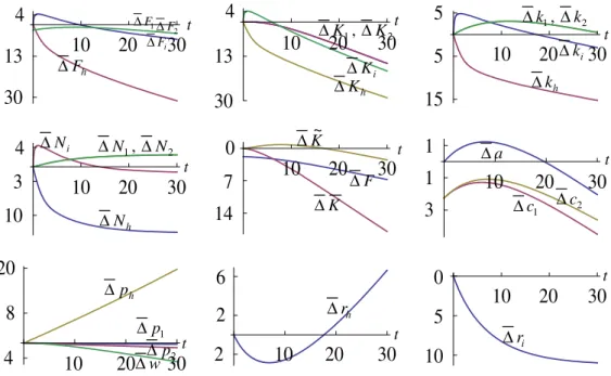
We now increase the propensity to save in the following way: .

77 . 0 75 . 0 :

0 ⇒

λ The results are plotted in Figure 2. In the plots, a variable

( )

t

x_j

dynamic effects of the change in the same parameter may be different. The labor input of the heavy industrial sector fall and the labor inputs of the two service sectors rise. The labor input of the light industrial sector rises initially but falls in the long-term. The rate of interest on the heavy capital goods falls initially but rises in the long-term; correspondingly the stock of the heavy capital goods rises initially but falls in the long-term. The rate of interest on the light capital goods falls.

Figure 2. A rise in the propensity to save

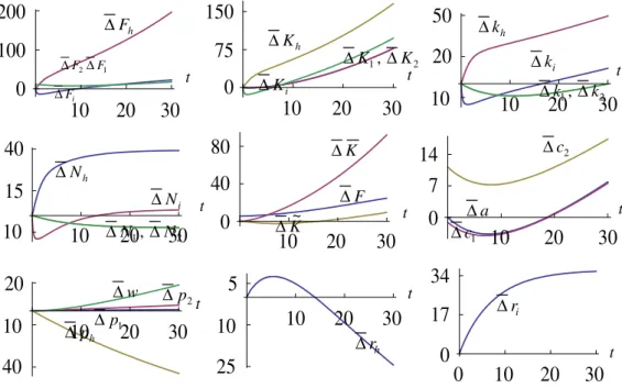
A rise in the propensity to consume service 2

We now increase the propensity to consume service 2: ξ₂₀:0.08⇒0.09. The results are plotted in Figure 3. As the household spends more on service 2, the consumption level of service 2 is increased. As the demand for the service is increased, the price of service 2 is increased. The supply of service is also increased. The wealth per capita and consumption level of service 1 are reduced initially but increased in the long term. The wage rate is increased in association with the rising price of service 2. The price of service 1 is changed but only slightly. The output levels of the two service sectors are increased. The output level of the light industrial sector falls initially but increased in the long-term. It should be noted that the output levels of the four sectors are all increased as the propensity to consume service 2 is increased. The labor inputs of the two service sectors fall and the labor input of the heavy industrial sector rises. The labor input

10 20 30

30 13 4

10 20 30

30 13 4

10 20 30

15 5 5

10 20 30

10 3 4

10 20 30

14 7 0

10 20 30

3 1 1

10 20 30

4 8 20

10 20 30

2 2 6

10 20 30

10 5 0 i

F

Δ

h

F Δ

t t

t t

t t

t

t

t

1

F

Δ

h

r Δ

i

r Δ

2

F

Δ

h

K ΔΔKi

2 1, K K Δ Δ

h

k Δ

i

k Δ

2 1, k k Δ Δ

h

N Δ

i

N

Δ ΔN₁, ΔN₂

F Δ K Δ K~ Δ

2 c Δ

1 c Δ a Δ

h

p Δ

w Δ

1 p Δ

of the light industrial sector fall initially but rise in the long-term. The stock of the heavy capital goods rises. The stock of the light capital goods falls initially but rises in the long term. The national output is increased over time. The rate of interest on the light capital good rises. The rate of interest on the heavy capital good falls initially but rises in the long-term.

Figure 3. A rise in the propensity to consume service 2

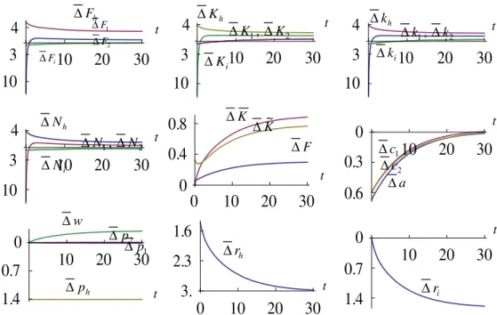
A rise in the depreciation rate of the heavy capital good

As different capital may depreciate differently, it is important to examine how the economic structural change takes place when a specified capital good depreciates more quickly. We now increase the depreciation rate of the heavy capital good: δ_h:0.05⇒0.051. The results are plotted in Figure 4. As the capital good depreciates more quickly, the stocks of the heavy and light capital goods are increased. The rates of interest on the capital goods fall in association with the rises in the capital stocks. The wage rate is increased, the prices of the two services are slightly changed. The heavy industrial sector’s output level is increased and the sector employs more labor. The national output level is increased. The consumption levels of the two services and wealth per capita are reduced initially but are affected only slightly in the long-term.

10 20 30 0

100 200

10 20 30

0 75 150

10 20 30

10 20 50

10 20 30

10 15 40

10 20 30

0 40 80

10 20 30

0 7 14

10 20 30

40 10 20

10 20 30

25 10 5

0 10 20 30

0 17 34

i

F

Δ

h

F Δ

t t

t t

t t

t _t

t

1

F

Δ

h

r Δ

i

r Δ

2

F

Δ

h

K Δ

i

K Δ

2 1, K K Δ Δ

h

k Δ

i

k Δ

2 1, k k Δ Δ

h

N Δ

i

N Δ

2 1, N N Δ Δ

F Δ

K Δ

K~ Δ

2 c Δ

1 c Δ

a Δ

h

p Δ

w Δ

1 p Δ

Figure 4.A rise in the depreciation rate of the heavy capital goods

A rise in the total productivity of the light industrial sector

We increase the total productivity factor of the light industrial sector in the following way: Ai:1.1⇒1.12. The rise in the total productivity of the light industrial sector initially leads to the falling in all the inputs of the sector. The three inputs are increased in the long-term. Correspondingly, the output level of the light industrial sector falls initially but rises in the long-term. The output level of the heavy industrial sector and the three inputs of the sector are increased over time. The output levels of the two service sectors and the three inputs of each sector are reduced initially but increased in the long-term. The stocks of the two capital goods are increased. The price of the heavy capital goods falls and the prices of the two services rise. The consumption levels of the two services fall initially but rise in the long-term. The national output and wealth per capita are increased over time.

10 20 30

10 3 4

10 20 30

10 3 4

10 20 30

10 3 4

10 20 30

10 3 4

0 10 20 30

0 0.4 0.8

10 20 30

0.6 0.3 0

10 20 30

1.4 0.7 0

0 10 20 30

3. 2.3 1.6

10 20 30

1.4 0.7 0

i

F

Δ

h

F Δ

t t

t t

t t

t

t

t

1

F

Δ

h

r Δ

i

r Δ

2

F

Δ

h

K Δ

i

K Δ

2 1, K K Δ

Δ Δkh

i

k Δ

2 1, k k Δ Δ

h

N Δ

i

N Δ

2 1, N N Δ

Δ _ΔF

K Δ

K~ Δ

2 c Δ 1 c Δ

a Δ

h

p Δ

w Δ

Figure 5.A rise in the total productivity of the light industrial sector

5. Conclusions

The history of economic growth theory shows that it is difficult to formally model economic dynamics with multiple capital goods and multiple consumption goods and services with micro-foundation. This paper proposed a two-capital-goods model to illustrate how economic growth with multiple capital two-capital-goods can be modeled with an alternative approach to household behavior. We also analyzed changes in the parameters upon the system. Our model shows the importance of introducing heterogeneous capital into the neoclassical growth theory. For instance, in our model when the propensity to save is increased, the wealth per capita is increased initially but reduced in the long-term and the wage rate and national output level fall; the consumption levels of the two services fall even though the prices of the two services fall only slightly; the stock of the light capital goods rises initially but falls in the long-term; the stock of the heavy capital goods falls in association with rising of in its price; the labor input of the heavy industrial sector fall and the labor inputs of the two service sectors rise while the labor input of the light industrial sector rises initially but falls in the long-term; the rate of interest on the heavy capital goods falls initially but rises in the long-term; correspondingly the stock of the heavy capital goods rises initially but falls in the long-term; the rate of interest on the light capital goods falls. Solow’s one-sector and Uzawa’s two-sector growth models cannot explain the structural changes with

10 20 30

24 7 10

10 20 30

25 10 5

10 20 30

25 10 5

10 20 30

25 10 5

0 10 20 30

0 1.5 3

10 20 30

1 0.5 2

10 20 30

0 1.2 2.4

0 10 20 30

0 3 6

10 20 30

0 3 6

i

F

Δ h

F Δ

t t

t

t t

t

t

1

F

Δ

h

r

Δ Δri

2

F

Δ

h

K Δ

i

K Δ

2 1, K K Δ

Δ Δkh

i

k Δ

2 1, k k Δ Δ

h

N Δ

i

N Δ

2 1, N N Δ Δ

F Δ

K

Δ ΔK~

2 c Δ

1 c Δ a Δ

h

p Δ

w Δ

1 p

Δ 2

p Δ

t

heterogeneous capital. Our model also predicts some phenomena which are different from what the standard one-sector growth model predicts. Both Solow’s one-sector and Uzawa’s two-sector growth models show that a rise in the saving rate will increase the wealth per capita both in the short-term and in the long-term, while our model predicts that as the propensity to save is increased, the wealth per capita is increased initially but reduced in the long-term. This occurs because the dynamic interdependence among the variables becomes more complicated in a model with heterogeneous capital than the one with homogeneous capital. It should be noted that the comparative dynamic analyses are conducted only with specified values of the parameters. If the parameter values are specified differently, the system may not have a stable equilibrium. We have limited our study to a simplified spatial structure of the economic system. There are numerous extensions of the Solow-Uzawa models. We may introduce more realistic representations of household behavior with endogenous time and multiple kinds of consumption goods. We now point out a few straightforward extensions. For instance, we may consider the economy as a small country, which implies that economy has negligible impact on the interest rate in globally open market. This assumption has been accepted in the literature of international economics.

Appendix 1. Proving Lemma 1

From (2), (4) and (6), we have

, , ... , 1 , , ,

ˆ ,

ˆ

J i

h m N

k z

N K Z

m m m

m m

m× = γ × =

α

= (A1)

where

. ˆ

, ˆ

m m m m m m

γ β γ α β

α ≡ ≡

From (2), (4) and (6), we also have

, , ... , 1 , , ,

ˆ

J i

h m K z k

m m m

m =

α × × γ

= (A2)

where zˆ = z/Z. From (3) and (4), we have

, ˆ

, ,

ˆ

i i

i i i

i i i

i i h h h

z f A r

f A w

Z f A

p r

δ − × × γ × γ =

× × β = ×

α × × α = δ × +

(A3)

7

(

)

.

ˆ ˆ

,

i i

i i

z Z z Z f

γ α

γ

α ⎟⎟_⎠

⎞ ⎜⎜ ⎝ ⎛ ⎟⎟ ⎠ ⎞ ⎜⎜ ⎝ ⎛ ≡

From (A3), we see that r_h + p_hδ_h, w, and r_i are functions of Z and .z From (A3) and (11), we solve

(

)

, .

ˆ

h i h h

i i i i

h r r p

r Z

f A

p =

δ +

× α × × α

= (A4)

From (5) and (6), we have

. ˆ ˆ

j j

j j

z Z A w p

j j

j j

j α γ

γ α

× × × β

γ × α ×

= (A5)

From (7) and (8), we have

(

)

(

1

)

~ .

ˆ r p k r k w

y = _h + _h + + _i + (A6)

From (4) and (6), we have

. , ... , 1

, j J

N p

F N F

i j j

i j i

j =

× × β

× × β

= (A7)

From (9) and (14), we have

. ˆ

j j j

p y N

F = ξ × × (A8)

From (A7) and (A8), we have

. , ... , 1 , ˆ

J j

F y N N N

i i

i j

j

j =

× β

× × × ξ × β

= (A9)

Insert (3) in (A9)

, , ... , 1 ,

ˆ j J

y

where we also use (A1) and

(

,

)

ˆ ˆ .

i i i i z Z A N z Z i i i i j j

j α γ

γ α × × × β γ × α × × ξ × β ≡ Λ

Insert (A10) in (12) , ˆ N y N

Nh + i +Λ = (A11)

where . 1

∑

= Λ ≡ Λ J j j

Insert (A1) in (13)

, ˆ

ˆ

ˆ 1 Z

K N N N J j j j i i h

h + +

∑

=

= α α α . ~ ˆ ˆ

ˆ 1 z

K N N N J j j j i i h

h _{+ +}

∑

₌

= γ γ

γ (A12)

Insert (A10) in (A12)

, ˆ ˆ ˆ Z K y N N h i i h

h _{+ + Λ =}

α α , ~ ˆ ˆ ˆ z K y N N i i i h

h _{+ + Λ =}

γ

γ (A13) where

(

)

(

)

. ˆ , , ˆ , 1 1

∑

∑

= = Λ ≡ Λ Λ ≡ Λ J j j j i J j j j

h Z z Z z

γ α

Insert (A6) in (A11) and (A13)

(

, ,

)

,

~ 1

1 K w

N p r N z Z K K N r N

N i h h

i

h ⎟Λ −Λ

⎠ ⎞ ⎜ ⎝ ⎛ + − ≡ Ω = Λ ⎟ ⎠ ⎞ ⎜ ⎝ ⎛ + + +

(

, ,

)

, ~ 1 ˆ

ˆ 2 N K w

p r Z K z Z K K N r N N h h h h h i i i h

h _{⎟Λ −Λ}

9

(

, ,

)

.

~ 1 1

ˆ ˆ

3 K w

N p r z

Z K

K z N

r N

N

i i

h h

i i

i i

h h

Λ − Λ ⎟ ⎠ ⎞ ⎜

⎝ ⎛ + − ≡ Ω

=

= ⎥ ⎦ ⎤ ⎢

⎣ ⎡

− Λ ⎟ ⎠ ⎞ ⎜ ⎝ ⎛ + + γ + γ

(A14)

This is a linear system with N_h, N_i, and K~ as variables. It is straightforward to solve this linear system as follows:

(

K,Z,z

)

, N

(

K,Z,z

)

, K~

(

K,Z,z

)

,

N_h = Ω_{h i} = Ω_i = Ω_k (A15)

where we do not provide explicit functions as it is straightforward to get them but the expressions are tedious. By the following procedure, the variables in the dynamic system can be expressed as unique functions of Z,z and K: Nh, Ni,

and K~ by (A15) ⇒ w and r_i by (A3) ⇒ p_h by (A4) ⇒ p_j, j =1,..., J, by

(A4)⇒ r_h by (A4) ⇒ yˆ by (A6) ⇒ N_j, j =1,..., J, by (A10) ⇒ K_m and

,

m

k m = h,i,1,..., J, by (A.1) ⇒ Fh by (1) ⇒ Fi by (3) ⇒ Fj,

, , ... ,

1 J

j = by (5) ⇒ c_j and s by (9) ⇒ a =

(

p_hK + K~

)

/N. We can thus

express the dynamics of (10) and (15) as follows:

( )

t 1

(

K, Z, z

)

s

( ) ( )

t at ,

a = Ψ ≡ −

( )

t 2

(

K, Z, z

)

F

( )

t K

( )

t , K = Ψ ≡ _h −δ_h

( )

(

, ,

)

( )

~

( )

. ~

3 K Z z F t K t

t

K = Ψ ≡ _i −δ_i (A16)

We will not give explicit expressions of Ψ_j

(

k,Z, z

)

as it is straightforward to have these expressions by the procedure above. Taking derivatives of

(

p K K

)

N

a = _h + ~ / with respect to time yields

,

3 2

N N

p z z p N K Z Z p N K

a h h ₊ hΨ ₊ Ψ

∂ ∂ + ∂ ∂

=  

 (A17)

where we also use (A16). Similarly from (A15), we have

. ~

2 z

z Z Z K

K k k  k _

∂ Ψ ∂ + ∂

Ψ ∂ + Ψ ∂

Ψ ∂

From (A16), (A17) and (A18), we have

,

3 2 1

K p N

z z p Z Z

p_{h h} Ψ − _hΨ −Ψ

= ∂ ∂ + ∂

∂ _{ }

.

2

3 Ψ

∂ Ψ ∂ − Ψ = ∂

Ψ ∂ + ∂

Ψ ∂

K z

z Z Z

k k

k  _{ (A19)}

This is a linear system with Z and z as variables. We solve (A19)

(

, ,

)

,

1 K Z z

Z = Ψ

(

, ,

)

.

2 K Z z

z = Ψ (A20)

(A16) and (A20) express Z, ,z and K as functions of K, Z and z.

Notes

(1)

A comprehensive survey on the early literature of growth theory is referred to Jones and Manuelli (1997). See Buirmesiter and Dobell (1970) and Zhang (2005) for the literature on the traditional neoclassical growth theory.

(2)

See, for instance, Drandakis (1963), Diamond (1965), Weizsäcker (1966), Corden (1966), Stiglitz (1967), Gram (1976), Benhabib and Nishimura (1981).

(3)

See also Baxter (1996), Erceg et al. (2005) and Fisher (2006).

(4)

The early extensions are referred to Takayama (1985) and Zhang (2005). Recent extensions include, for instance, Galor (1992), Azariadis (1993), Mino (1996), Drugeon and Venditti (2001), Harrison (2003), Cremers (2006), Herrendorf and Valentinyi (2006), Li and Lin (2008), and Stockman (2009).

(5)

In the rest of the paper we treat consumption good exchangeably with service.

(6)

It should be noted that before Uzawa published the two-sector growth model, there were some models of multiple sectors and heterogeneous capital (von Neumann, 1937, Koopmans, 1951, Morishima, 1964). See also Takayama (1985) and Dolmas (1996) for the literature review.

(7)

Moreover, labor is not explicitly considered in the model.

(8)

1

References

Acconcia, A., Simonelli, S. (2008). “Interpreting Aggregate Fluctuations Looking at Sectors”,

Journal of Economic Dynamics & Control, 32, pp. 3009-3031 Azariadis, C. (1993). Intertemporal Macroeconomics, Oxford: Blackwell

Baxter, M. (1996). “Are Consumer Durables Important for Business Cycles?”, The Review of Economics and Statistics, 78, pp. 147-155

Benhabib, J., Nishimura, K. (1981). “Stability of Equilibrium in Dynamic Models of Capital Theory”, International Economic Review, 22, pp. 275-293

Burmeister, E., Dobell, A.R. (1970). Mathematical Theories of Economic Growth, London: Collier Macmillan Publishers

Corden, W.M. (1966). “The Two Sector Growth Model with Fixed Coefficients”, Review of Economic Studies, 33, pp. 253-263

Cremers, E.T. (2006). “Dynamic Efficiency in the Two-Sector Overlapping Generalizations Model”, Journal of Economic Dynamics & Control, 30, pp. 1915-1936

D’Agata, A. (2009). “Endogenous Adaptive Dynamics in Pasinetti Model of Structural Change”,

Metroeconomica, 60, pp. 1-31

Diamond, P.A. (1965). “Disembodied Technical Change in a Two-Sector Model”, Review of Economic Studies, 32, pp. 161-168

Dolmas, J. (1996). “Endogenous Growth in Multisector Ramsey Models”, International Economic Review, 37, pp. 403-421

Drandakis, E. (1963). “Factor Substitution in the Two-Sector Growth Model”, Review of Economic Studies, 30, pp. 105-118

Drugeon, J.P., Venditti, A. (2001). “Intersectoral External Effects, Multiplicities & Indeterminacies”, Journal of Economic Dynamics & Control, 25, pp. 765-787

Erceg, C., Guerrieri, L., Gust, C. (2005). “Can Long-run Restrictions Identify Technology Shocks?”, Journal of European Economic Association, 3, pp. 1237-12878

Farmer, K., Wendner, R. (2003). “A Two-Sector Overlapping Generations Model with Heterogeneous Capital”, Economic Theory, 22, pp. 73-92

Harrison, S.G. (2003). “Returns to Scale and Externalities in the Consumption and Investment Sectors”, Review of Economic Dynamics, 6, pp. 963-976

Herrendorf, B., Valentinyi, A. (2006). “On the Stability of the Two-Sector Neoclassical Growth Model with Externalities”, Journal of Economic Dynamics and Control, 30, pp. 1339-1361 Fisher, J.D.M. (2006). “The Dynamic Effects of Neutral and Investment-Specific Technology

Shocks”, Journal of Political Economy, 114, pp. 413-451

Galor, O. (1992). “Two-sector Overlapping-generations Model: A Global Characterization of the Dynamical System”, Econometrica, 60, pp. 1351-1386

Gram, H.G. (1976). “Two-Sector Models in the Theory of Capital and Growth”, The American Economic Review, 66, pp. 891-903

Jones, L., Manuelli, R.E. (1997). “The Sources of Growth”, Journal of Economic Dynamics and Control, 21, pp. 75-114

Kaganovich, M. (1988). “Sustained Endogenous Growth with Decreasing Returns and Heterogenous Capital”, Journal of Economic Dynamics and Control, 22, pp. 1575-1603 Koopmans, T.C. (1951). Analysis of Production as an Efficient Combination of Activities, in

Kurz, M. (1963). “The Two Sector Extension of Swan’s Model of Economic Growth: The Case of No Technical Change”, International Economic Review, 4, pp. 1-12

Li, J.L., Lin, S.L. (2008). “Existence and Uniqueness of Steady-State Equilibrium in a Two-Sector Overlapping Generations Model”, Journal of Economic Theory, 141, pp. 255-275 Meade, J.E. (1961). A Neoclassical Theory of Economic Growth, London: Allen and Unwin Mino, K. (1996). “Analysis of a Two-Sector Model of Endogenous Growth with Capital

Income Taxation”, International Economic Review, 37, pp. 227-251 Morishima, M. (1964). Equilibrium, Stability, and Growth, Oxford: Claredon Press

Solow, R. (1956). “A Contribution to the Theory of Growth”, Quarterly Journal of Economics, 70, pp. 65-94

Solow, R.M. (1962). “Note on Uzawa’s Two-Sector Model of Economic Growth”, Review of Economic Studies, 29

Stiglitz, J.E. (1967). “A Two Sector Two Class Model of Economic Growth”, Review of Economic Studies, 34, pp. 227-238

Stockman, D.R. (2009). “Chaos and Sector-Specific Externalities”, Journal of Economic Dynamics and Control, 33, pp. 2030-2046

Takayama, A. (1985). Mathematical Economics, Cambridge: Cambridge University Press Uzawa, H. (1961). “On a Two-Sector Model of Economic Growth I”, Review of Economic Studies,

29, pp. 47-70

Uzawa, H. (1963). “On a Two-Sector Model of Economic Growth I”, Review of Economic Studies,

30, pp. 105-118

von Neumann, J. (1937). “A Model of General Economic Equilibrium”, translated from the German origin, Review of Economic Studies, 33 (1945-6), pp. 1-9

Weizsäcker, C.C. (1966). “Tentative Notes on a Two-Sector Model with Induced Technical Progress”, Review of Economic Studies, 33, pp. 245-251

Whelan, K. (2003). “A Two-Sector Approach to Modeling US NIPA Data”, Journal of Money,

Credit and Banking, 35, pp. 627-656

Zhang, W.B. (1996). “Preference, Structure and Economic Growth”, Structural Change and Economic Dynamics, 7, pp. 207-221

Zhang, W.B. (2005). Economic Growth Theory, Hampshire: Ashgate

Zhang, W.B. (2012). “Economic Structural Change and Growth with Two Capital Goods”,