❊♥s❛✐♦s ❊❝♦♥ô♠✐❝♦s
❊s❝♦❧❛ ❞❡
Pós✲●r❛❞✉❛çã♦
❡♠ ❊❝♦♥♦♠✐❛
❞❛ ❋✉♥❞❛çã♦
●❡t✉❧✐♦ ❱❛r❣❛s
◆◦ ✹✹✾ ■❙❙◆ ✵✶✵✹✲✽✾✶✵
❆ ▼♦❞❡❧ ♦❢ ❈❛♣✐t❛❧ ❆❝❝✉♠✉❧❛t✐♦♥ ❛♥❞ ❘❡♥t✲
❙❡❡❦✐♥❣
P❛✉❧♦ ❇❛r❡❧❧✐✱ ❙❛♠✉❡❧ ❞❡ ❆❜r❡✉ P❡ss♦❛
❏✉♥❤♦ ❞❡ ✷✵✵✷
❖s ❛rt✐❣♦s ♣✉❜❧✐❝❛❞♦s sã♦ ❞❡ ✐♥t❡✐r❛ r❡s♣♦♥s❛❜✐❧✐❞❛❞❡ ❞❡ s❡✉s ❛✉t♦r❡s✳ ❆s
♦♣✐♥✐õ❡s ♥❡❧❡s ❡♠✐t✐❞❛s ♥ã♦ ❡①♣r✐♠❡♠✱ ♥❡❝❡ss❛r✐❛♠❡♥t❡✱ ♦ ♣♦♥t♦ ❞❡ ✈✐st❛ ❞❛
❋✉♥❞❛çã♦ ●❡t✉❧✐♦ ❱❛r❣❛s✳
❊❙❈❖▲❆ ❉❊ PÓ❙✲●❘❆❉❯❆➬➹❖ ❊▼ ❊❈❖◆❖▼■❆ ❉✐r❡t♦r ●❡r❛❧✿ ❘❡♥❛t♦ ❋r❛❣❡❧❧✐ ❈❛r❞♦s♦
❉✐r❡t♦r ❞❡ ❊♥s✐♥♦✿ ▲✉✐s ❍❡♥r✐q✉❡ ❇❡rt♦❧✐♥♦ ❇r❛✐❞♦ ❉✐r❡t♦r ❞❡ P❡sq✉✐s❛✿ ❏♦ã♦ ❱✐❝t♦r ■ss❧❡r
❉✐r❡t♦r ❞❡ P✉❜❧✐❝❛çõ❡s ❈✐❡♥tí✜❝❛s✿ ❘✐❝❛r❞♦ ❞❡ ❖❧✐✈❡✐r❛ ❈❛✈❛❧❝❛♥t✐
❇❛r❡❧❧✐✱ P❛✉❧♦
❆ ▼♦❞❡❧ ♦❢ ❈❛♣✐t❛❧ ❆❝❝✉♠✉❧❛t✐♦♥ ❛♥❞ ❘❡♥t✲❙❡❡❦✐♥❣✴ P❛✉❧♦ ❇❛r❡❧❧✐✱ ❙❛♠✉❡❧ ❞❡ ❆❜r❡✉ P❡ss♦❛ ✕ ❘✐♦ ❞❡ ❏❛♥❡✐r♦ ✿ ❋●❱✱❊P●❊✱ ✷✵✶✵
✭❊♥s❛✐♦s ❊❝♦♥ô♠✐❝♦s❀ ✹✹✾✮
■♥❝❧✉✐ ❜✐❜❧✐♦❣r❛❢✐❛✳
A Model of Capital Accumulation and Rent-Seeking
∗
Paulo Barelli
†Samuel de Abreu Pessôa
‡June, 2002
Abstract
A simple model incorporating rent-seeking into the standard neoclassical model of capital ac-cumulation is presented. It embodies the idea that the performance of an economy depends on the efficiency of its institutions. It is shown that welfare is positively affected by the institu-tional efficiency, although output is not necessarily so. It is also shown that an economy with a monopolistic rent-seeker performs better than one with a competitive rent-seeking industry.
JEL ClassiÞcation: D23, D74, O40, O41, O47
Key Words: Rent-seeking, Two Sector Model, Capital Accumulation, Productivity
“Economic history may be thought of as a struggle between a propensity for growth and one for rent-seeking, that is, for someone improving his or her position, or a group bettering its position, at the expense of the general welfare. (...) Whenever conditions permitted, that is, when rent-seeking was somehow curbed, growth manifested itself.” (Jones,1988)
“Institutions form the incentive structure of a society, and the political and economic institutions, in consequence, are the underlying determinants of economic performance.” (North, 1994)
∗
Rafael Rob read a previous version of this paper. His comments and suggestions were essential for making the text clear. Evidently, errors are the sole responsibility of the authors.
†
Department of Economics, Columbia University, 420 W118th Street, New York, NY10027, USA. Email Address: pb230@columbia.edu
‡
Graduate School of Economics (EPGE), Fundação Getulio Vargas, Praia de Botafogo190,1125, Rio de Janeiro, RJ, 22253-900, Brazil. Fax number: (+) 55-21-2553-8821. Email address: pessoa@fgv.br
1
Introduction
It is not a novelty to claim that the performance of an economy is shaped by its institutions. Douglass North and others have published several books and papers on the subject. The argument goes as follows. Institutions are the rules of the game in an economy. If these rules foster activities that generate high private beneÞts and low social beneÞts, then the economy performs poorly. Conversely, if the rules align private and social beneÞts, economic growth and high social welfare result. Economic activities can, then, be classiÞed according to the relation between private and social beneÞts generated by each activity. To simplify matters, let us assume that there are only two types of economic activities: those that generate social returns, and those that do not. The institutional background will be considered efficient if it fosters relatively more of the Þrst type of activity. This simpliÞcation summarizes the argument set forth in the literature mentioned above. In this paper a model capturing the ideas above is presented. It is a standard neoclassical capital accumulation model with intertemporal consumers, with the introduction of an additional, rent-seeking, industry. That is, economic activities are classiÞed into two economic sectors: a productive and an unproductive. Both employ productive factors to produce an output, but the second’s output is an effort to conÞscate what is produced by theÞrst. Such a formulation seems to capture the idea of an activity with private beneÞts and no social beneÞts. It is a pure transfer activity, that only redistributes income (does not generate it).1 The Þrst activity, on its turn, does
generate income - its output is the socially valued homogeneous good in the economy.
The introduction of the new industry is made by the use of a function, which we interpret as the ‘aggregate rent-seeking technology.’ This function translates the output of the unproductive sector into a number between 0 and1, which represents the fraction of the productive sector’s output that is captured by the unproductive sector. This function is the central piece of the model. A set of properties that such a function ought to satisfy is presented,2 and it is shown that these properties
are sufficient to close the model. In particular, no functional form is needed to solve the model. As it is the case with production functions, functional forms are only necessary for some applications (and our function does have a ‘Cobb-Douglas-like’ counterpart that is used to calibrate the model). We argue, in addition, that such a function is a natural way of incorporating institutions into a macroeconomic model.
The institutional efficiency is captured by the above mentioned function. The fraction of sector
1Such an activity is also called a rent-seeking activity, as coined by Krueger (1974), or a directly unproductive
proÞt-seeking (DUP) activity, as coined by Bhagwati (1982).
2We assume, in particular, that the shape of the function is one that delivers uniqueness of equilibrium. It is
1’s output that sector 2 is able to conÞscate depends on how well property rights are enforced. We introduce one institutional parameter that determines the success of sector 2’s output in capturing sector 1’s output. It can be viewed as a measure of the total factor productivity in that sector. A low value for this parameter makes unproductive activities relatively unsuccessful in their endeavor of capturing sector 1’s output, so it represents well deÞned property rights. A high value for the parameter represents an inefficient institutional background, i.e., poorly deÞned property rights. This parameter is the main maintened assumption of the model - it is the exogenous variable that eventually drives all results. The view set forth by the model is, then, that of an economic long-run in which the institutional efficiency is held Þxed, so that the “long-run” does not include institutional change.
With two sectors there are also two economic decisions: one static and the other dynamic. The static is the factor allocation problem (for a given level of productive factors), and the dynamic is the consumption-investment allocation problem (that is, endogenous levels of reproductive factors of production). In both an equilibrium is deÞned and shown to exist and be unique. The effect of the institutional efficiency can also be disentangled into a static and a dynamic parts. That is, for a given level of productive factors, the institutional efficiency determines the amount of resources employed in the rent-seeking sector, i.e., employed with a view to capture rents. This is similar to Gordon Tullock’s idea, and we will call it the Tullock effect accordingly. Moreover, the institutional efficiency also generates a dynamic effect, that of a distortion in capital accumulation. This is the usual effect of a distortion, and will be called the Harberger effect.3 These two effects summarize the workings of the model.
There are two central results in this paper. First, welfare is positively related to institutional effi -ciency. Second, a monopolist rent-seeker is better for the economy than a competitive rent-seeking sector. The Þrst result, although intuitive, is by no means obvious. The long-run comparative statics indicates that there is no monotonic relation between per capita output and institutional efficiency. In particular, if the rent-seeking sector is capital intensive, then worse institutions might be associated with more output in the long-run. The welfare result states that, even when long-run output and consumption do increase, society is negatively affected by a worsening in institutional efficiency. Moreover, the effect of a change in institutional efficiency on welfare can be disentangled
3We named the two effects Tullock and Harberger because they resemble the Tullock/Harberger debate of the social costs of monopoly. Harberger pointed out that the cost of the monopoly is the deadweight loss it generates, and found out that this loss is small. Tullock replied saying that the monopolist captures part of consumers’ surplus, and hence that real resources would be employed to capture these economic rents, so the cost of a monopoly is much larger than the deadweight loss it generates. Hence, our Tullock effect measures the resources used to capture rents, and our Harberger effect measures the usual cost of inefficient institutions (the dynamic distortion). Posner (1975) evaluated empirically the Harberger and Tullock effects for a monopoly in a partial equilibrium framework.
into two effects, which correspond to the Tullock and Harberger effects mentioned above. The unambiguous result can be interpreted as the Tullock effect dominating the Harberger effect when the latter happens to be of opposite sign (the Tullock effect is always of the same sign: the worse the institutions, the more is captured by the rent-seeking sector. The Harberger effect can be of the opposite sign when rent-seeking is capital intensive). Hence, the fact that productive resources are employed in unproductive activities is the main cause of welfare being reduced because of inefficient institutions.
The second result is important because it qualiÞes the claim that competition is always to be recommended. Competition in productive sectors does indeed improve welfare. But competition in unproductive sectors generates the opposite effect. As several producers compete for rents, they employ more productive resources and generate more unproductive output than a sole rent-seeker would generate.4
This helps explain the events that ensued from three different historical phenomena of the second half of last century: the end of European colonization in the 60’s and 70’s in many African countries, the end of political regimes based on military dictatorship in many Latin America countries in the 80’s, and Þnally the ‘fall of the wall’ leading to the end of the communist regimes in east Europe in the late 80’s and early 90’s. These three recent episodes of the world history share one fundamental characteristic: there is a transition from a centralized political (economic) organization toward a more decentralized system. And such transitions were all accompanied by a period of economic recession. One rationale for that is provided by our second result above. That is, assuming that monopoly in rent-seeking takes place in either a colony (the European imperial power being the monopolist),5 or in a military dictatorship (the army being the monopolist), or a centralized
economy (the communist party being the monopolist), a given level of institutional efficiency is associated with a better economic performance in the more centralized system as compared to a system in which there is free entry into the rent-seeking sector (for two otherwise identical economies, of course). Also, the transition to a more open system of organizing either the politics or the economy means a lifting of the barriers to entry in the rent-seeking sector, so the economy is bound to experience a recession as productive resources are directed to unproductive activities.6
4Shleifer and Vishny (
1993) make this point informally. Bliss and Di Tella (1997) study the link between corruption and competition. Their model differs from our formulation in many aspects: (i) they consider competition in the productivity activity but monopoly in the rent-seeking sector; (ii) they examine a partial equilibrium set up (there is no factor mobility); (iii) they do not consider capital accumulation.
5Lucas (
1990) considered the case in which the European power is the monopolist in the capital market. 6
Some qualitative results are presented as well. For the static part, an increase in the capital stock leads to an increase (decrease) in sector 2’s relative output when sector 1 is capital (labor) intensive. This is the expected result: when the rent-seeking industry is labor intensive, more capital means more output and hence a bigger pool to be robbed. On its turn, a worsening in the institutional set leads unambiguously to an increase in the relative size of the rent-seeking industry as expected. For the long-run, one would expect that when sector1is capital intensive, a worsening in the institutional set would lead to a reduction in capital and output. And this is indeed the case. But when sector 2 is capital intensive, the expected results do not necessarily take place. One would expect that a worsening in the institutional set would lead to more capital and less output, but we cannot rule out the cases where capital decreases and/or output increases. The results depend on values of parameters and we argue that, for the empirically relevant values, the expected results do emerge.7
Features of the transitional dynamics are also considered. If the rent-seeking sector is labor intensive the model delivers the usual dynamics of the neoclassical model of capital accumulation: both capital stock and output increase. On the other hand, if the rent-seeking sector is capital intensive, capital stock may increase and output may decrease along the transition. Arguably, the rent-seeking sector is labor intensive since it produces a service. However the opposite case can be illustrated by some African countries. For such countries it is reasonable to assume that the rent-seeking sector is the capital intensive one, since the productive sector is mostly agricultural and the rent-seekers are mostly armed bands and the army itself, and indeed these economies present positive investment and a decrease in output. In this way the model offers one rationale for the recent experience of such countries. Observe that such result is similar to the immizerizing growth literature, but not exactly the same. It states that capital accumulation generates less output because capital is mainly employed in unproductive activities. Immizerizing growth, on its turn, comes from capital accumulation generating a deterioration in the terms of trade that more than offsets the positive effects of the former.
Finally, some quantitative implications of the model are considered. First, the model is cal-ibrated using explicit functional forms. We use data on per capita income and a measure of institutional efficiency both from Hall and Jones (1999). The model Þts the data quite well. The
functioning legal system that enforces contracts (and also, clearly, on economic relations based on contracts). Every such aspect ought to be considered in the transition. What our model says is that any such institutional change is reßected in our institutional parameter. Indeed, all those changes lead in one way or the other to an improvement in the protection of property rights, and this is captured by our institutional parameter. (See Svejnar (2002) for an exposition of the transition in the former Soviet economies.)
7Although the indeterminacy is somewhat counter-intuitive, it shows that there is more to the model than just
‘bad institutions causing bad economic performance.’
calibration exercise illustrates that a monopolist rent-seeker is signiÞcantly better than a compet-itive rent-seeking industry to the economy. Second, it is shown that the model can be used to explain income differences among countries based only on incentives. In fact, for this task the model performs quite similarly to the neoclassical model with a high capital share. It is well known that one needs a capital share in excess of 23 for the latter model to explain differences in income (see Lucas (1990), Barro and Sala-i-Martin (1995) and Mankiw (1995)). The model presented here explains those differences with a capital share of 13, which is consistent with the observed one. Since the model is an extension of the neoclassical model, one can argue that it not only introduces rent-seeking in a standard macroeconomic model, it also makes that model more congruent with the observed data. One reason why a high capital share is needed in the neoclassical model is that all factors of production are assumed to be employed in productive activities. Once this assumption is relaxed, there is no need for a high (and unrealistic) capital share. In other words, the model provides a rationale for lower TFP among poorer economies, where the share of production factors allocated in the productive activity can be viewed as an “endogenous TFP.”8
The paper is organized as follows. The model is presented in section 2. The assumptions behind the aggregate rent-seeking technology are given, and the static and dynamic equilibria are deÞned. Section 3 shows the existence and uniqueness of these two equilibria. Section 4 presents the comparative statics results, and also the properties of the transition dynamics. The two central results are shown in sections 5 and 6, and in section 7 the quantitative results are presented. Section 8 relates our work with the previous literature and section 9 concludes with some remarks about possible extensions and applications of the model.
2
The Model
The model presented in this paper can be viewed as a simple extension of the neoclassical model of capital accumulation. In that model, there is just one good produced by a constant returns to scale technology employing capital and labor, whose services are rented by a representative consumer
8As Prescott (
to the Þrms. The representative consumer makes her intertemporal decision optimally taking into account the income stream she will receive from her renting of those services. Institutions are usually introduced, in a macroeconomic setup, as a wedge between what Þrms produce and the income they earn. That is, output of theÞrms is summarized by an aggregate production function, F(K, L), andÞrms’ income is given by a fraction of that output, (1−τ)F(K, L). The ‘tax rate’τ
represents any sort of distortion that might characterize the economy, which could be a tax itself. In general, it can be identiÞed with the efficiency of the institutional background of the economy. The simple extension considered here is to give a speciÞc formulation for the ‘tax rate’τ.
In particular, it will be assumed that there exists another sector in the economy, called the unproductive sector (also the rent-seeking sector, or sector 2). Like the productive sector (sector
1), it combines capital and labor to produce an output, but this output is not another good. It is a service, a transfer service. That is, an effort to conÞscate goods produced in sector 1. The more service is produced, the larger the amount of goods that gets transferred toward sector 2. Calling Y1 and Y2 the output levels of sectors1 and 2 respectively, the idea above can be stated as
follows: sector 1 keeps (1−τ(Y2))Y1 and sector 2 is able to conÞscateτ(Y2)Y1 goods from sector
1, where τ is an increasing function of the transfer services, Y2. Formally, the burden imposed by
the rent-seeking sector on the productive sector is a negative externality, which would not emerge if property rights were fully enforced. This is not the case by the very nature of the rent-seeking problem.
The functionτ will be fully derived and characterized below (it will be denoted byg to reserve the symbol τ for a bona Þde tax rate). This function g is the main analytical contribution of the model presented here. As mentioned above, the standard way of introducing institutions in a macroeconomic model is via something like g, so it seems natural to suggest a characterization of such entity. To the best of our knowledge, though, no such characterization has been provided yet. In this section the production side of the economy will be presented, including the function g mentioned above. The two-sector structure allows one to deÞne a static equilibrium, the equilibrium allocation of productive factors between the two sectors. This equilibrium is characterized and some interpretations are given. Then the demand side of the economy is presented using the standard intertemporal representative consumer. The long-run equilibrium is then considered. Finally, both equilibria are shown to exist and be unique under the maintained assumptions.
2.1
Firms
2.1.1 P r oduct i ve Sect or
The productive sector consists of N1 identical Þrms9 operating under the same technology and
producing a single commodity, called ‘the good.’ Firm i (i ∈ N1) combines capital, K1i, and
labor, L1i, according to a constant returns to scale technology F1, to produce output Y1i. That
is, Y1i ≡ F1(K1i, L1i). Part of what this Þrm produces is captured by the Þrms operating in
the unproductive sector. In other words, from the point of view of the productive sector, the unproductive activity acts like a tax rate τ on its output, so Þrm i keeps only (1−τ)Y1i of its
output. Under perfect competition, Þrmi’s program is to
max K1i,L1i
(1−τ)Y1i−r1K1i−w1L1i,
where r1 and w1 are the rental and wage rates prevailing in sector1.
The Þrst order conditions are given by
r1 = (1−τ)f10(k1), (1)
w1 = (1−τ) £
f1(k1)−k1f10(k1) ¤
, (2)
where f1≡F1(k1,1)and k1 ≡ KL11ii, which are the same for any Þrm.
The total output of sector 1 is denoted byY1 and is given byY1 = Pi∈N1Y1i. The per capita output is y1 ≡ YL1 =l1f1(k1), where L is the population and l1 ≡ L1 Pi∈N1L1i is sector 1’s labor share.
2.1.2 A ggr egat e Rent -Seeki ng
From the technological point of view, the major distinction between the productive activity and the unproductive one is that in order to ‘produce’ unproductive output it is required capital and labor services, and output. The productive activity, on its turn, requires only capital and labor services. Let G be the total amount of output which is extracted from the productive sector by the unproductive sector. We assume that G= G(θY2, Y1), where the function G is homogeneous
of the Þrst degree,Y2 is the total output of transfer services, andθis an institutional variable that
describes the quality of the institutional set. A high (low) θ represents a bad (good) institutional background. We viewθ as a measure of ‘total factor productivity’ (TFP) of sector 2, and henceθ
9
enters as an argument of GmultiplyingY2. From the homogeneity ofG,one can write
G=g
µ
θY2
Y1 ¶
Y1 =g¡θyR¢Y1, (3)
where y2≡ YL2, yR = yy21, and g ³
θY2
Y1
´
≡G(θY2
Y1 ,1).The function g is the share of the output of the productive sector that is extracted by the unproductive sector.10 As anticipated above, the share
g is precisely the tax rate τ thatÞrms in sector 1take as given:
g¡θyR¢=τ.
The formulation states, therefore, that the aggregate rent-seeking technology, g, must be a function of the relative output y2
y1 multiplied by an institutional variable θ. It is reasonable to assume that g(0) = 0 and g0(x) > 0, for any x ≥ 0. In addition, for it to be a share, it will be
assumed thatlimx→∞(x) = 1. Any functiong satisfying these properties can be used to introduce rent-seeking in the neoclassical capital accumulation model.11 In this paperg will be assumed to
satisfy the following four axioms as well. Letαg ∈(0,1)be given, and deÞne αg(x)≡xg
0(x)
g(x)1−1g(x).
Let also α1L be sector1’s labor share on income.
Axiom 1 limx→0g0(x) =∞and g00(x)<0.
Axiom 2 0<αg(x)≤αg.
Axiom 3 αg <α1L.
Axiom 4 g(x) = 1+m(x)m(x) for some ms.t. m0(x)>0, m00(x)<0, m(0) = 0,limx
→0m0(x) =∞. Axiom 1 is the standard Inada condition plus strict concavity, and is what ensures uniqueness of equilibrium. Such an assumption reßects our view that development issues are to be explained by differences on the fundamentals among economies, and not by coordination failures.12 The term
10
The function G plays, in the context of rent seeking, the role of the matching function in the equilibrium unemployment literature. (See Mortensen and Pissarides,1994.) Theregis the rate that seekers of job position meet vacancies; heregis the rate that the seekers of rents exploit the productive sector. Although one activity, job search, is productive and the other, rent-seeking, is not, the formal properties of the function gare the same.
1 1Observe that the function g can be viewed as a cumulatitive distribution function, and issues of risk aversion
could be considered as well. We do not pursue this line of reasoning here as the setup is assumed deterministic.
12Of course, multiplicity of equilibria can be introduced by relaxing the strict concavity assumption. This would lead to the issue of indeterminacy of equilibrium and of coordination failures. Such phenomena belong, in our view, to short to medium run macroeconomic theories. In the very long run, what matters is the more fundamental properties of an economy. We would not argue, for instance, that Brazilian GDP isÞve times smaller than the American one
αg is an upper bound forαg(x). Axiom 2 states thatαg(x)must be strictly less than one. Ifαg = 1 (< 1), the aggregate rent-seeking technology is said to present constant (decreasing) returns to scale.13 Observe that ifα
g happens to be constant then integrating αg(x) yields
g(x) = x
αg
1 +xαg, (4)
which is one candidate for a functional form14 forg. Axiom 3 is needed for long-run stability and
is only used in that section of the model. It ensures saddle-path stability of the dynamic system.15
Finally, Axiom 4 ensures uniqueness of equilibrium in the monopoly formulation (section 6), and it is needed only for that section. In particular, the main model (the competitive one) is solved for a generic function g satisfying Axioms1, 2, and 3.
2.1.3 U n pr oduct i ve F i r m
The unproductive sector consists of N2 (endogenously determined) identicalÞrms operating under
the same technology and producing a single service, called transfer service. Firm i (i ∈ N2)
combines capital, K2i, and labor, L2i, according to a constant returns to scale technologyF2, to
produce output Y2i ≡ F2(K2i, L2i). The quantity of goods that this particular Þrm expropriates
from the productive sector is a share of the total booty G in (3). It is assumed that this share is of the additive Contest Success Function (CSF) form,16 so that it can be written as P h(θY2i)
j∈N2h(θY2j).
That is, Þrmiwill Þght for a share of Gand the success of such a Þght will be determined by the CSF. It is again reasonable to assume that h(0) = 0 and h0(x) >0, for any x≥ 0. We will make
one further assumption.
Axiom 5 There exists a unique x¯ such thatarg maxxh(x)x = ¯x.
In other words, there exits one, and just one, optimal scale for eachÞrm in sector 2. Observe that Axiom 5 does not posit uniqueness of a point where marginal returns equal average returns, it only asks that there exists just one point that maximizes average returns.
because of some unlucky choice of equilibrium. The structure of incentives (institutions) in Brazil is clearly less efficient than the American one. (Evidently, coordination failures, history dependence, or political economy issues can help understanding why these bad institutions were adopted in one place and not in other. See for instance Engerman and Sokoloff(1997).)
13This denominations are explained in the static equilibrium section.
14Observe the analogy with the Cobb-Douglas functional form.
15
The termαg(x) is the normalized elasticity ofg(x). It was introduced here becauseαg(x)<α1L is the stability condition. The functional form (4) is a useful by-product.
16
The analysis is made on the limit in which there are many Þrms in each sector so that the Dixit-Stiglitz (1977) assumption of discharging terms that depend on N11 or N12 from theÞrst order conditions can be made.17,18 Consequently, Þrmi’s program
max K2i,L2i
h(θY2i) P
j∈N2h(θY2j) g
µ
θ
P
j∈N2Y2j Y1
¶
Y1−r2K2i−w2L2i, (5)
generates the following Þrst order conditions:
r2 =
θh0(θY2i) P
j∈N2h(θY2j)
g¡θyR¢f20(k2)Y1, (6)
w2 =
θh0(θY2i) P
j∈N2h(θY2j)
g¡θyR¢ £f2(k2)−k2f20(k2) ¤
Y1. (7)
2.1.4 Fr ee Ent r y
In keeping with the competitive paradigm, equilibrium within each sector is achieved when each Þrm makes zero proÞt. It follows from (1) and (2) that π1i = 0 for any i ∈ N1 (hence N1 is
indeterminate). For sector 2, substituting (6) and (7) into (5) yields
π2i = h(
θY2i) P
j∈N2h(θY2j)
g¡θyR¢Y1 µ
1−θY2ih 0(θY2i)
h(θY2i) ¶
, (8)
which is not necessarily zero. Here is where Axiom 5 plays a role. Setting Y2i = x¯θ in (8) yields
π2i= 0 (becauseh0(¯x) = h(¯¯xx)), so this level of Y2i for every Þrm in sector 2 is an equilibrium with
free entry. It is unique by hypothesis.19
Substituting the free entry condition π2i = 0 into (6) and (7), it follows that a symmetric
17The attentive reader will have noticed that we have already make this assumption in deriving (
1) and (2): since
τ =g³θY2
Y1
´
, to takeτ as given amounts to assume away the effect of a particularÞrm in sector1onY1. 18
Consequently, we are assuming that the optimum size of a Þrm in sector 2, x¯, is small enough such that in equilibrium N2 is large.
19It is also a Nash equilibrium for the game played by the
Þrms in sector 2. That is, assume each Þrm plays x¯ and consider Þrm i contemplating playing x 6= x¯ instead. Straightforward com-putations yield π2i = (N2−1)hh(( ¯xx)) +h(x)g
³
θy2
y1
´
Y1 − r2K2i−w2L2i. Substituting (6) and (7) yields π2i = h(x)
(N2−1)h( ¯x) +h(x)g
³
θy2
y1
´
Y1³1−xhh0(( ¯xx))´<0,soÞrmiwill not deviate.
equilibrium20 is given by
r2 =
g¡θyR¢
yR f 0
2(k2), (9)
w2 =
g¡θyR¢ yR
£
f2(k2)−k2f20(k2) ¤
. (10)
2.2
Static Equilibrium
The static equilibrium is an equilibrium in the allocation of productive factors between the two sectors, for given levels of productive factors and institutional efficiency (k and θ). We use the underlying two-sector structure of the model to deÞne such equilibrium. The idea is that each combination of output levels of both sectors determines a marginal rate of transformation and is in turn determined by the latter. The equilibrium is a Þxed point of this mutual determination.
More speciÞcally, each allocation of productive factors generates some output levelsy1 and y2
and consequently a marginal rate of transformation of g(θyyRR)1−g(1θyR) of goods into transfer services.
The term g(θyyRR) represents a change in sector 2’s output, and the term 1−g ¡
θyR¢represents a
change in sector1’s output. The ratio is a feasible reallocation of productive factors. On the other hand, a marginal rate of transformation (MRT) also deÞnes output levelsy1 and y2. Indeed, using
the underlying two-sector structure, one can write yi(p, k) as sector i’s static supply function,21
wherepis the slope of the PPF, i.e., the MRT. That is, each MRT corresponds to one point on the PPF. The static equilibrium is deÞned as apthat is self-determining in the above sense, so that it is given by the following Þxed-point:
p= g ¡
θyR(p, k)¢
yR(p, k)
1
1−g(θyR(p, k)) ≡H(p, k,θ). (11)
2.3
Interpretation
The production side of the economy was presented above. The characterization of the ‘tax rate’ τ
as a function g representing the aggregate rent-seeking technology was made under fairly general conditions. The two-sector structure provides a characterization of the static equilibrium in terms of equation (11).
From now on as an abuse of languageyi(p, k), i= 1,2,will be called the supply of goods and unproductive services andpthe relative price of the unproductive service in units of goods. Observe
2 0Recall that for a symmetric equilibrium h(θY2 i) PN 2
j = 1h(θY2 j) = 1
N2.
21Appendices A.1and A.2 provide a short review of the static two-sector general equilibrium model. See chapter
that in this economy to produce one unit of good does not mean to be the owner of it. There are, therefore, three goods in this two-sector economy: the good, the rent-seeking service, and the good at somebody’s hands. The price p1 = 1−g is the relative price of one unit of the good in units
of goods at somebody’s hands, and p2 = ygR is the relative price of one unit of the rent-seeking
service in units of goods at somebody’s hands. By construction, y1 =p1y1+p2y2, so one can view
p1y1+p2y2 as total output of the economy in units of goods at somebody’s hands.
The static equilibrium can be understood as a consequence of factor mobility. With mobility and interior solution, it must be that r1=r2 and w1 =w2, otherwise all productive factors would
be allocated in just one of the industries. From the two-sector general equilibrium model, we know that
ri=pifi0(ki) (12)
wi=pi £
fi(ki)−kifi0(ki) ¤
, (13)
where pi is the price of sectori’s output, i= 1,2. It follows from comparing (1), (2), (9), and (10)
to (12) and (13), that the static equilibrium is given byp1 = 1−g and p2 = yy12g, which is what is expressed in (11). If p > H(p, k,θ) (p < H(p, k,θ)) then factors will move towards sector 2 (sector
1), reducing (increasing)p and increasing (reducing) H because sector 2 (sector 1) pays relatively more. In equilibrium, factor prices are equalized and there is no further factor reallocation.
The static equilibrium condition (11) establishes the allocation at each point in time of capital and labor between the two sectors. It can be written as
g(θy2
y1
) = p2y2
p1y1+p2y2
. (14)
The LHS of (14) can be written as gy1
gy1+(1−g)y1, which is the ratio between the ‘output’ of the unproductive sector, gy1, and the total output, y1. The RHS of (14) can be written as (rkrk+2+ww)l2,
which is the ratio between the remuneration of the factors employed in the unproductive sector and the total factor remuneration. The short-run equilibrium is the allocation that equalizes the relative output of the unproductive sector with its relative income. In other words, given that there is free entry in both industries, the equilibrium condition is that average beneÞt equals average cost.
2.4
Consumers
At a point in time, that is, for given values forkandθ,the static model is solved yieldingp,yi(p, k), and the factor pricesr and w. The representative household rents her capital and labor services to
the Þrms. She chooses a consumption plan that solves
max c(t)
∞
Z
0
e−ρtu(c(t))dt
s.t. k(·t) = (r(t)−δ)k(t) +w(t)−c(t),
given k(0), whereρis the intertemporal discount rate, and δ is the physical depreciation rate. This is the standard Ramsey problem that yields the following Euler equation
·
c(t) =c(t)γ(c(t)) (r(t)−ρ−δ), (15)
whereγis the intertemporal elasticity of substitution, andr= (1−g(θyR(p, k))f0
1(k1(p))as derived
before.
From the two-sector model it is known that per capita income equals per capital output, i.e., that
r(t)k(t) +w(t) =p1(t)y1(t) +p2(t)y2(t) =y1(t), so that the dynamics are represented by the following dynamic system22
·
k=y1(p, k)−c−δk
·
c=cγ(c)
¡1−g(θyR(p, k))¢f10(k1(p))
| {z }
r
−ρ−δ
, (16)
together with the initial condition for capital,k(0), and the terminal conditionlimt→∞e−ρtu0(c(t))k(t) = 0, wherep=p(k,θ) is the short-run equilibrium,
The condition for saddle point stability of (16) is that the Jacobian of the linearized system be negative, and this boils down to
k r
dr dk
¯ ¯ ¯ ¯θ=
µ
g αg
1−αg
− 1 α2K
k2
k1−k2 ¶
k p
∂p
∂k
¯ ¯ ¯
¯θ <0. (17)
Appendix B.1shows that Axiom 3 is a sufficient condition for the inequality above to hold.
2 2
2.5
Long Run Equilibrium
The long-run equilibrium is given by a capital stock and a relative price that satisfy the conditions of a steady-state of the dynamic system (16). In other words, the following system of equations must hold in the long-run:
ψ1(p, k) = g(yθyRR(p,k)(p,k))1−g(θy1R(p,k))−p= 0
ψ2(p, k) =¡1−g(θyR(p, k))¢f0
1(k1(p))−(ρ+δ) = 0.
(18)
3
Existence and Uniqueness
In this section it is shown that both static and long-run equilibria exist and are unique. Such results complete the set up of the model. The properties and applications of the model will be presented in the following sections. Letpandpbe the prices under which the economy is specialized in sector
1 and 2 respectively.23
Proposition 1 The short-run equilibrium exists and is unique.
P r oof . LetH : [p, p]→R+be the mapping deÞned byH(p)≡H(p, k,θ)for given(k,θ),so that
the short-run equilibrium p(k,θ) is given by aÞxed point of H. Taking derivatives and rearranging:
p H(p)
dH(p)
dp =−(1−αg)
p yR(p)
dyR(p)
dp <0,
and the inequality follows from αg <1. From Axiom 1 we havelimp→p+ H(p) = limyR→0
g(θyR) yR ≥ limyR→0g0
¡
θyR¢=∞.From Axiom 2, integratingα
ggivesg(x)≤ x
αg
1+xαg. Hencelimx→∞x(1−g(x))
≥limx→∞ x
1+xαg =∞, which ensures that limp→pH(p) = limyR→∞
g(θyR)
yR 1−g(1θyR) = 0.
Observe that if instead ofαg <1one hadαg = 1,then if one point on the PPF is an equilibrium
any other one is also an equilibrium. That is why this case was called constant returns to scale on aggregate rent-seeking. Finally, ifαg >1there is still a unique interior equilibria, which is unstable
(the two corners become stable).
Proposition 2 The long-run equilibrium exists and is unique.
2 3For a given level of factor endowment k, p ≥ p(k) (p ≤ p(k)) means that the economy is specialized in the production of rent-seeking services (sector1’s good). Note thatp0(k)≷0andp0(k)≷0ask1≷k2.
P r oof . Let f0
1(kρ+δ) = ρ+δ and ψ1(pρ+δ, kρ+δ) = 0. Given that on p(k) the economy is
specialized in the production of the productive good,
r|(p(k
ρ+δ),kρ+δ) =ρ+δ⇒
¡
p(kρ+δ), kρ+δ
¢
∈[ψ2= 0].
Additionally, we know thatr = (1−g)f0
1|(pρ+δ,kρ+δ)∈ψ1 <ρ+δ.In order to show that there is a point
on ψ1 = 0 such that r=ρ+δ we show that limp→0r=∞.Given Axiom 2, write αg(x)≤αg−ε,
for some ε>0. From (17)
p r
dr
dp =g
αg 1−αg
− α1L
1−α2K−α1L ≤ αg 1−αg
− α1L
1−α1L ≤ −β,
where β ≡ (1−α ε
1L)(1−α1L+ε) > 0. Let (p0, k0) ∈ ψ1, and let r0 = (1−g)f
0
1|(p0,k0). Integrating the
last inequality yields
r r0
≥
µ p
p0 ¶−β
,
for any p ≤ p0. This shows existence. For uniqueness, notice that since 0 > ddrk¯¯θ = ∂∂rk¯¯p,θ +
∂r
∂p ¯ ¯ ¯k,θ ddkp
¯ ¯ ¯ψ
1,∗
, and ddpk¯¯¯
ψ2,∗=
−
∂r
∂k|p,θ ∂r
∂p
¯ ¯ ¯
k,θ
,we have
dp
dk
¯ ¯ ¯ ¯
ψ2,∗ =
∂r
∂k ¯ ¯
p,θ ∂r
∂k ¯ ¯
p,θ−
dr
dk ¯ ¯
θ
dp
dk
¯ ¯ ¯ ¯
ψ1,∗
≶ dp
dk
¯ ¯ ¯ ¯
ψ1,∗
as k1 ≷k2,
so the curves intersect only once.24
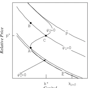
The idea of the proof is shown by Figures1and 2 below. They represent the systemψ1(p, k) = 0
and ψ2(p, k) = 0when the production functions are Cobb-Douglas and the aggregate rent-seeking function is given by (4). (The curve ψM1 = 0 refers to the monopoly solution of the mod-els. See section 6.) Figure 1 considers sector 1 as capital intensive (the parameter values are
{α1,α2,αg,θ,δ,ρ} = {1/3,1/6,1/8,1,log(1.066),log(1.03)}) and in Figure 2 sector 1 is labor
in-tensive (the parameters are{1/6,1/3,1/8,10,log(1.066),log(1.03)}). As it is clear from theÞgures,
ψ1(p, k) = 0 andψ2(p, k) = 0must intersect once, and only once.
2 4Recall that dp
dk
¯ ¯
k* k r+d
Capital
p*
e
vit
al
e
Re
ci
r
P
B
A
C y1=0
y2=0 p—
p
y1M=0
Figure 1: Sector1 capital intensive
k* k
r+d
Capital
p*
e
vit
al
e
Re
ci
r
P
A B
C y2=0
y1=0 p—
p y1M=0
Figure 2: Sector 1labor intensive
4
Properties of the Model
4.1
Comparative Statics
4.1.1 Shor t -R un
From (11), the effects ofkand θ on the static equilibriump are given by
k p
∂p
∂k
¯ ¯ ¯ ¯
θ
=−
(1−αg) ykR
∂yR
∂k ¯ ¯ ¯ p
1 + (1−αg) ypR
∂yR
∂p ¯ ¯ ¯k
≷0 ask1 ≷k2, (19)
θ
p
∂p
∂θ
¯ ¯ ¯ ¯k=
αg 1 + (1−αg) ypR
∂yR
∂p ¯ ¯ ¯k
>0. (20)
Hence the comparative statics in the short-run are as follows: an increase in the per capita capital stock leads to more unproductive activity when sector1is capital intensive, and to less unproductive activity when sector 1 is labor intensive. The former case can be thought of as the case in which capital is a valuable resource in the economy (a good). The more of it, the better for both sectors. Sector 1 produces more and sector 2 is able to appropriate more (the “pie” increases, so more to everybody.) For the latter case (k1< k2), capital is less valued than labor (it is a bad). An increase
in k is effectively a reduction in the relative supply of labor, so it is harmful for sector1 (and for sector 2 consequently). The effect of the institutional variable does not depend on the technologies: the worse the institutional background, the bigger the unproductive sector.
4.1.2 Long-R un
In the long-run capital is endogenous and given by (18). The only exogenous variable is θ, the variable that captures the efficiency of the institutional background. When sector 1 is capital intensive the results are intuitive: a worsening in institutional efficiency generates less capital and output in the long-run. But when the rent-seeking sector is capital intensive, then the reverse result cannot be ruled out. That is, it can be that as the institutional background becomes worse, long-run income increases. Since this counter-intuitive effect does not seem to correspond to any relevant empirical evidence, it is qualiÞed in terms of parameter values. In particular, for it to happen, it is necessary that sector 2 be signiÞcantly more capital intensive than sector 1. In particular, Appendix C.5 shows that
α2K ≤min np
l1,(1 +σ1)α1K o
(21)
is a sufficient condition to rule out a counter-intuitive effect ofθ ony1. Observe that (21) is likely
to take place. There is no available data for α2K, but σ1 and α1K are known to be close to1 and 1
3 respectively. l1 is the share of the labor force employed in the productive sector, which is also
something not available. Tentatively, let us say that l1 is close to 14, so that three fourths of the
workers are employed as rent-seekers. Even in this case,α2K would have to be bigger that 12, which
seems unlikely since the overall capital share is close to 13.
4.2
Features of the Dynamics
If the economy is not at its long-run equilibrium, it is at a transition path of capital accumulation. In what follows, it is shown that an economy might be in a dynamic path of capital accumulation with a decreasing level of output.
In Appendix B.2 it is shown that
dy1
dk
¯ ¯ ¯ ¯θ =
∂y1
∂k
¯ ¯ ¯ ¯p+
∂y1
∂p
¯ ¯ ¯ ¯k
∂p
∂k
¯ ¯ ¯
¯θ >0 (22)
if k1 ≥k2.That is, one can only guarantee that output is increasing along the transition if sector
1 is capital intensive. Analogously, it is also possible to show that dy2
dk ¯ ¯ ¯
θ > 0 if k1 ≤ k2. More
speciÞcally, in Appendix B.2 it is shown that ddykR¯¯¯
θ ≶ 0 as k1 ≷ k2, i.e., that the ratio
y2
y1 is monotone in k: increasing if rent-seeking is capital intensive and decreasing otherwise. Also, the same pattern is followed by the relative value of sector 2’s output, py2
y1+py2.
rent-seeking sector is capital intensive. Although this conÞguration is uncommon - the rent-rent-seekingÞrm produces a service and services are usually labor intensive - it is not only a theoretical possibility. Take a very underdeveloped economy (from sub-Saharan Africa for instance). Its productive sector is the agricultural sector. Its unproductive sector is the army and armed bands. It makes sense, then, to consider the rent-seeking sector as the capital intensive sector for this economy. Many sub-Saharan countries have been experiencing negative growth rates and positive investment. One way of explaining it is that investment has been directed mainly to unproductive activities. As an example, in Appendix B.2 it is shown that, for the extreme case that the productive sector only employs labor (α1K = 0), the condition 1>(1−αg)σ2 is sufficient to ensure that ddyk1
¯ ¯
¯θ <0, and
this is the case as long as 0 ≤ σ2 ≤ 1, which is by no means a strong assumption. Hence, if an
economy can be characterized by the above parameters, the condition ensuring positive investment and negative growth is that the elasticity of substitution in sector 2 be not larger than 1.
In the next section a welfare analysis will be presented. It is the analysis of the impact of θ
on welfare, and not the effect of capital accumulation on welfare. While the latter can be negative (immizerizing), it is shown that the former cannot.
5
Welfare Analysis
The results above show that properties of the model capture a variety of possible phenomena. The fact that the long-run comparative statics depend on the underlying factor intensity is viewed as a positive feature of the model, since one can, then, use the model to explain different phenomena. But this dependency on factor intensity might be viewed as an indeterminacy. Such is not a concern when the welfare analysis is considered. There is a monotone relation between institutional efficiency and overall welfare in the economy. The worse the institutional background, the lower the welfare enjoyed by the representative consumer. The relevant criterion for evaluating economic performance is welfare, and under such criterion the variable θ does represent the “underlying determinants of economic performance,” as North would put it.
A worsening in the institutional set of the economy generates two effects. First, an increase inθ
increasesp (see (20)) producing an inßow of factors toward the rent-seeking sector and a reduction on the productive sector’s output. This is the called the Tullock effect. Second, from (1), an increase in θ increases the distortion to capital accumulation. This is called the Harberger effect. Under the assumption that initially the economy is in long-run equilibrium, it is shown that (i) it is possible to disentangle the welfare effect in two components, which are the two above mentioned effects, (ii) the marginal impact of a reduction on institutional efficiency is a reduction in welfare, and (iii) if both sectors operate under the same technology the Harberger effect is zero.
Given that the economy is a representative agent economy, the intertemporal utility is the social welfare function. In order to evaluate the welfare impact of a marginal increase in θ, taken into consideration the transitional dynamics, a technic developed by Judd (1982 and1987) is employed. Let W =R0∞e−ρtu(c(t))dt be the welfare index. The impact of θ on W at steady state (denoted
by an *) is:
dW dθ ¯ ¯ ¯ ¯ ∗ = Z ∞ 0
e−ρtu0(c(t))¯¯
∗ dc(t)
dθ dt=u
0(c∗ )
Z ∞
0
e−ρtdc(t)
dθ dt=u
0(c∗
)Cθ(ρ),
where Xθ(ϑ)≡R
∞ 0 e
−ϑtdx(t)
dθ dt is the Laplace transform of
dx(t)
dθ for any functionx(t).
Hence, the effect on welfare is given by the Laplace transform (Cθ(ρ)) of ddc(t)θ multiplied by
marginal utility evaluated at c∗
. In appendix C.1it is shown that
ρCθ(ρ) = dy1
dθ
¯ ¯ ¯ ¯k,∗ | {z } Tullock Effect
+µ−ρ
µ
c∗ γ(c∗
)
ρ d
r dk ¯ ¯θ,∗
ρ+δ− dy1
dk ¯ ¯ ¯θ,∗+ c
∗γ(c∗)
ρ d
r dk ¯ ¯θ,∗
Ã
dy1
dk
¯ ¯ ¯
¯θ,∗−ρ−δ ! dk dθ ¯ ¯ ¯ ¯∗
| {z }
Haberger Effect
, (23)
where µ is the positive eigenvalue associated with the matrix of the linearized dynamic system. Hence, the impact of θ on welfare is given by the sum of two terms that are identiÞed as the Tullock and Harberger effects.
The Tullock effect is given by the instantaneous reduction on output, and consequently on consumption, resulting from the deterioration of the institutional set and the corresponding increase in the relative size of the rent-seeking industry. Under any conÞguration the Tullock effect is negative (see (20)).
The Harberger effect is the composition of two terms. One is the net marginal impact of capital accumulation on output (net of physical depreciation and of the intertemporal opportunity cost of
investment), Ã
dy1
dk
¯ ¯ ¯
¯θ,∗−ρ−δ ! dk dθ ¯ ¯ ¯
¯∗. (24)
The other is the attenuation factor (AF), which translates a change in output due to capital accumulation into a change in welfare taking into consideration the transitional dynamics,
AF= µ−ρ
µ
c∗ γ(c∗
)
ρ d
r dk ¯ ¯θ,∗
ρ+δ− dy1
dk ¯ ¯ ¯θ,∗+ c
∗γ(c∗)
ρ d
r dk ¯ ¯θ,∗.
Note that limγ→0AF = 0 and limγ→∞AF = limγ→∞µ −ρ
µ = 1. In Appendix C.2 it is shown that 0≤AF≤1. Appendix C.4 shows that the Tullock effect is larger than the net marginal impact of capital accumulation on output (24). Consequently,
dW dθ
¯ ¯ ¯ ¯
∗ <0,
i.e., the effect on welfare of a change in the institutional background is unambiguous: welfare is reduced when institutions get less efficient.25
This is the main qualitative result of the model. It makes a case for improving efficiency of institutions of property rights enforcement based on welfare grounds. Alternatively, it states that the main problem of an unproductive activity is that it employs productive resources that could have been employed socially valued activities. This is the main driving force behind the result that welfare depends positively on institutional efficiency.
Remark 1 Appendix C.3 shows that, even when the economy is not initially at a steady state
postition, we still have dW
dθ <0. Better still, the impact ofθ on welfare can always be decomposed
into Tullock and Harberger effects, and these two effects combined are always negative.
Finally, Appendix B.2.2 shows that
dy1
dk
¯ ¯ ¯
¯θ,∗−ρ−δ ≷0 ask1 ≷k2,
so, from (24), the Harberger effect is zero if k1 =k2.26
6
Monopoly
The model presented in this paper assumes that the rent-seeking sector is a competitive industry. The free entry condition and the assumption of an optimum plant size for each Þrm in sector 2 guarantee that rents are fully dissipated in equilibrium. It seems reasonable to assume that proÞt
2 5
Observe an analogy of (23) with the Slutsky equation of consumer theory: a change in θ may be viewed as a change in the price of the consumption good. The total effect is then separated into the substitution effect (the Tullock effect, always of the right sign) and the income effect (the Harberger effect, which has ambiguous sign). What is shown is that the substitution effect always dominates the income effect making the consumption good an “ordinary” good.
2 6Under this conÞguration (k
1 = k2) it follows from the short-run equilibrium condition (14) that the share
of workers in the rent-seeking sector, l2, is equal to the share of output extracted by the rent-seeking sector, g. Consequently, the marginal impact of capital on output,l1f0(k), is equal to the market interest rate,(1−g)f0(k),
and the social value of capital is equal to the private one.
opportunities will be taken up by someone in a society, so the assumption of a large number of rent-seekers has its appeal. It is plain that different forms of market organization could be considered. We decided to stick to the competitive paradigm because we view it as the relevant scenario for a market economy, especially in the long-run. In this section, the model with just one Þrm operating in sector 2 is considered.27 With such a model, one can compare the results of the previous model
and also, as was argued in the Introduction, compare the effects of rent-seeking in open societies with rent-seeking in more closed societies.
It is possible to imagine a situation in which there is a central organization that gives right to a unique Þrm to practice rent-seeking.28 Assume that this central organization does exist and that
it is able to enforce this right.29 The monopolist uses its market power to make positive proÞts30 and generates less rent-seeking than a competitive industry does.
The monopolist problem is to solve
max K2,L2
g
µ
θL2f2(k2)
Y1 ¶
Y1−r2K2−w2L2,
which yields
r2 =θg0¡θyR¢f20(k2)
w2 =θg0¡θyR¢ £f2(k2)−k2f20(k2) ¤
.
These two equations replace (9) and (10) for the competitive economy.
The argument to characterize the static equilibrium is the same as before. The marginal rate of transformation determined byyR is now θg
0(θyR)
1−g(θyR) and, for each given MRT, the relative pricepM
determines the relative supply yR, so that the equilibrium is aÞxed point as before31
HM(pM)≡ θg
0¡θyR¡pM¢¢ 1−g(θyR(pM)) =p
M.
2 7By doing that we analyze the two polar cases of market organization. Other market structures are likely to
generate conclusions lying somewhere in between the two extreme cases.
2 8As was argued in the Introduction, one can imagine that this monopolist is an Imperial European power, or a
military government, or the communist party. 2 9We can think, instead, that there are many
Þrms which are working as a cartel, maximizing jointly their proÞt. The key hypothesis here is limited entry in the rent-seeking sector.
3 0In order to close the model in general equilibrium we can think that each individual in the society is the owner
of an equal share of the rent-seekingÞrm, such that the proÞt is redistributed back to the household in a lump-sum fashion.
Strict concavity ofg implies that, for a given level ofθyR,g0¡θyR¢< g(θyR)
θyR ,or that HM(p)<
H(p). Under Axiom 4 it is straightforward to show that ∂H∂pM¯¯¯
k<0. Given that H
M(pM)¯¯
ψ1=0 <0
it follows that HM(pM)−pM = 0 lies somewhere in the middle of the stripe connecting ψ1 = 0
and p(k) (see Figures 1 and 2, where is it depicted as the curve ψM1 = 0). Consequently, a Þxed pointpM ofHM must be smaller that the equilibrium price of the competitive model: pM < p.This implies that
y1¡pM(θ, k), k¢> y1(p(θ, k), k).
Hence, for given values ofk and θ(that is, in the static part), a monopoly in sector 2 is better for sector 1. Less output gets conÞscated by sector 2. In other words, monopoly in the rent-seeking sector is better for the economy than competition in that sector. Competition improves welfare as long as it is employed in productive sectors of an economy. In an unproductive sector, given that competitors do not internalize the reduction in aggregate output due to their action, competition means too much production of transfer services, and consequently too much taken way from the productive sector and too much productive factors allocated in unproductive activities.
The long-run part is as before. The same intertemporal decision leads to a dynamic system like (16) with pM instead of p. Consequently, the long-run equilibrium is described by the crossing of
ψ2 = 0 and ψM1 = 0 in Figures 1 and 2. Given that ψ2 = 0 crossesψ1 = 0 and intersects p(k) at kρ+δ, existence follows from the same argument as before. Appendix D shows that even taking into
consideration the long-run endogenous capital adjustment we still have that monopoly is better:
y1M(θ)> y1(θ).
This result is far from immediate. The monopoly solution also delivers ambiguous results in the long-run comparative statics with respect toθ, so one could expect that the ambiguity would carry on to the comparison between yM
1 and y1. It turns out that this is not the case, and that the
short-run result holds in the long-run as well. The relatively smaller monopoly’s output is a beneÞt for the economy as a whole, as overall output (GDP) is larger.
At this point it is possible to analyze the transition from centralized political or economic systems to more open systems.32 Consider an economy in long-run equilibrium with monopoly in sector 2 (point A at Figure 1or 2). Following a change of system, the economy jumps to B, where it begins a dynamic path toward C, the long-run equilibrium for competitive rent-seeking and the same θ.33 The jump from A to B represents an unambiguous decrease in output. Given that
3 2
See the discussion in the Introduction.
3 3Notice that A might lie to the right of point C when sector 2 is capital intensive.
output in C is lower than output in A and that along the path from B toward C output is lower than output in A it follows that welfare reduces after the introduction of competitive rent-seeking.
7
Quantitative Implications
7.1
A Calibration Exercise
In this section the model is solved with particular functional forms and observed data is used to compute the implied values for the relevant parameters. The idea is to show how well the modelÞts the data and also to illustrate the difference between the competitive and monopoly solutions. We assume that the two sectors operate under the same technology (Cobb-Douglas with parameter α) and that the aggregate rent-seeking technology is given by the “Cobb-Douglas-like” form (4). With equal technologies it follows that yR = l2f(k)
l1f(k) ≡l
R. The long-run equilibrium condition becomes
αkα−1
1+(θlR)αg =ρ+δ.The short-run condition for the competitive economy is given byθ
αg¡lR¢αg−1
= 1, and for the monopoly is given by θαg(θl
R)αg−1
1+(θlR)αg = 1.
At this stage, two parameters are not observable in principle,θandαg. Instead of calibrating the
Þrst, we use a proxy for it. Given that it is meant to be a measure of the quality of the institutions of an economy, there is an observed variable that measures such a parameter. It is the variable SI (social infrastructure) created by Hall and Jones (1999), which is an index of institutional efficiency ranging from 0 to 1,1 being the highest degree of institutional efficiency. We assume that
θ=B1−SI SI ,
where B has to be calibrated. In other words the observable counterpart for θ is an increasing mapping on R[0,1] of the observable SI with an adjustable Jacobian given by B. So now the set {B,αg} of parameters has to be calibrated, and for that two observables are needed.
The Þrst observable comes from Anderson (1999). He reports that the aggregate burden of crime in the US is around 10% of GDP. Under the extreme assumption that rent-seeking in the US is mainly crime (US is indeed one of the most efficient economies in the world, so one might think of that assumption as a normalizing assumption that sets US’s institutional inefficiency outside crime to zero) we considerlR,US = 0.10.9 = 19,or lU S1
l1N N = 9
10, where the superscript NN stands for ‘neoclassical
nirvana,’ which is the situation with θ = 0. According to the data set of Hall and Jones (1999),
SIUS = 0.973. Given that the long-run solution of the competitive model is y U S
yN N = µ
1 +θ
αg
1−αg
¶ 1 α−1
and assumingα= 13,we get
B= 0.973 1−0.973
h (0.9)−2
3 −1
i1−αg
αg
. (25)
A second observable is needed to match the curvature parameter αg. Hall and Jones (1999)
estimated the equationlogyi =β0+β1SIi+²i.Their estimate forβ1 is 5.14. We therefore consider
αg as the solution of the following problem:
min
αg,ζ
1 Z
0
ζ+ 5.14SI−log "
1 + µ
B1−SI SI
¶ αg
1−αg
# 1 α−1
2
d(SI),
whereBis given by (25).34 That is, we considerαg that minimizes the distance betweenζ+ 5.14SI
and the logarithm of the income when θ is given byB1−SI
SI . The solution isαg = 0.506, which is
well inside the stability region of αg <1−α= 23.
Figure 3 below is the scatter diagram of the Hall and Jones data set for SI and per capita income,35 together with the long-run solution of the model with α
g = 0.506 and B = 1.391. It
is apparent that the pattern of the data is reproduced by the model. There is a negative relation between institutional inefficiency and output as expected. The fact that theÞt is a good one shows that the model can potentially explain the data.
Figure 4 displays the prediction of the model under the two conÞgurations: competitive seeking and monopoly. It is apparent that the competitive formulation generates much more rent-seeking for each level ofθ(or SI). This is in line with the interpretation that the monopoly solution is better for the rest of the economy.36
3 4
The constant ζ is an unimportant level parameter. Notice that we could have calibratedαg directly from the
data but we decided to use Hall and Jones’s regression because they controlled for endogeneity of SI. 3 5
The values of per capita income are net of mining activities as a way of controlling for natural resources and refers to the year of1988. Further data information can be found in their paper.
3 6
In Figure 5 we assumed that the monopoly economy is as good as the competitive rent-seeking economy in producing the good (that is, we assumed that the TFP of the Þrst sector is the same in both models). Although this is not true for either a centralized economy or a colony under European rule or a Latin American military dictatorship, we assumed it in order to isolate the differences in economic performance caused only by the form of market organization in the rent-seeking sector.
0 0.2 0.4 0.6 0.8 1
S.I.
5 10 15 20 25 30 35
y
-1
Figure 3
0 0.2 0.4 0.6 0.8 1
S.I.
5 10 15 20 25 30 35
y
-1
Competition
Monopoly
Figure 4
7.2
Explaining Income Di
ff
erences Using Incentives
The aim of this section is to show that the model presented here is capable of explaining the observed income inequality among economies. The driving force is, of course, the rent-seeking formulation, that incorporates in the same framework a distortion to capital accumulation and a displacement of productive factors away from the productive sector (which emulates a reduction in the TFP). That is, the Harberger and Tullock effects. The relevance of such capability stems from the fact that the standard neoclassical model is not able to explain the observed income inequality unless one makes some questionable assumptions. In particular, usually the capital share is assumed to be in excess of 23 (although it is a well established fact that such a share is close to 13). This model37
will be taken as the benchmark. It is characterized by y1 = f1(k) and y2 = 0, which mean that
there is a link between capital and output:
dy1
y1 =
α1Kdk
k . (26)
In a long-run situation such that, after allowing for risk, taxation, and other distortions, one has equalization of interest rates among economies, it is the case thatr =T f0
1(k) =constant, where T
stands for any distortion to capital accumulation as before. Consequently,
dr r =
dT T −
1−α1K
σ1
dk
k = 0. (27)
3 7See Mankiw (