Econ. Apl. vol.11 número4

(1)

Econ. aplic., São paulo, v. 11, n. 4, p. 507-525, ouTuBRo-DEZEMBRo 2007

New evideNce oN the determiNaNts of the gap

betweeN child support awards aNd child

support receipts*

regina madalozzo§

resumo

Cientistas sociais e planejadores de políticas públicas documentaram mudanças bastante significativas na estrutura familiar nos Estados Unidos nas últimas três décadas. Neste artigo, analisamos o grau de cumpri-mento de ordens de pensão alimentícia para crianças – significando a diferença entre o valor estipulado e o valor efetivamente pago – usando a base de dados da SIPP de 1990-1993. Exploramos os fatores que deter-minam a existência do gap, bem como sua dimensão, usando um modelo probit. Os resultados sugerem que tanto a existência quanto a magnitude, o gap, são positivamente influenciadas pelo tipo de acordo firmado entre os pais da criança.

palavras-chave: pensão alimentícia, modelo probit, economia da família.

abstract

Social scientists and policymakers have documented dramatic changes in the structure of US families over the past decades. In this paper, I analyze the child support compliance gap- the difference between expected payments and received child support payments- using a unique data set from the 1990-1993 SIPP on child support agreements. I explore the factors that determine the existence and the magnitude of a gap in payments using a probit model and regression analysis. Results suggest that both the existence of and magnitude of the child support gap are positively influenced by non-voluntary agreements received by the custodial parent.

Key words: child support, probit model, family economics.

Jel classification: J12, J13.

* I am grateful to the seminar participants at University of Illinois at Urbana-Champaign and Ibmec-SP, and to Kevin Hallock, John Johnson, Roger Koenker, Anil Bera, Werner Baer, and Dawn Nicholson for helpful comments. Financial support from Capes – Brazil is acknowledged. CPNq for research support through the Productivity on Research Fellowship, process number 306693/2004-6.

§ Professora Assistente no Ibmec São Paulo. E-mail: [email protected]. Adress for contact: Rua Quatá, 300, 4º andar, São Paulo, SP, CEP: 04546-042.

(2)

508 New evidence on the determinants of the gap between child support awards and child support receipts

Econ. aplic., 11(4): 507-525, out-dez 2007

1 i

NtroductioN

Social scientists and policymakers have documented dramatic changes in the structure of US families over the past three decades. Divorce rates rose dramatically between 1970 and 1980, but stabilized more recently, dropping to 4.3 percent by 1996. (U.S. Census Bureau, 2000). Over the same period, there was an increase in the number of single parent headed households. In 1970, only 12% of the children under 18 years old lived with one parent; by 1990, 25% of children lived in a single parent headed household. (U.S. Bureau of the Census, 1999). It is interesting to note that more than 57% of the black children under 18 years old live with only one parent (U.S. Department of Commerce, 1998). Policymakers have been concerned with these trends because living in a sin-gle parent household has been shown to have negative consequences for children, increasing the probability of teen pregnancy and of becoming a high school dropout (McLanahan and Sandefur, 1992). Single parent families are also linked to poverty. In 1996, 44.3% of the persons living in families with a female householder with no spouse present, and residing with related children were below the poverty level. (U.S. Census Bureau, 1997).

By late 1970’s and early 1980’s, the U.S. Government focused attention on the issues involving children in single-parent homes, including their well being and ways to move these groups above the poverty level. The passage of the Title IV-D of the Social Security Act in 1975 was designed to decrease dependence on welfare programs, particularly AFDC (Aid to Families with Dependent Children). At the same time, the federal government shifted responsibility for the collection of child support to the states. (Beller and Graham, 1993). The result of this shift was the establishment of new child support guidelines by more than half of the states by 1989. By the late 1980s, legislation concerning paternity establishment, income withholding and medical support orders were in effect in almost every state. (Garfinkel, McLanahan and Robins, 1994).

The impact of these various state level legislative programs has been the focus of research by several authors. Sorensen and Halpern (1999) use Current Population Survey (CPS) data and detailed information at the state-level to conclude that stronger child support enforcement has sig-nificant effect on child support receipts. Nixon (1997) also uses CPS data, but her focus is on the effects of child support enforcement on marital breakup. She found out that tougher child support enforcement reduces marital disruption.

Prior research on child support enforcement has concentrated on the levels of government ex-penditure on and efficiency of new programs, the impact of increased child support on labor force participation rates of men and women, and measurement of compliance rates. Another question frequently asked is why non-resident parents do not pay previously agreed to child support awards (Beller and Graham, 1993), and how some behaviors, as visitation frequency and both parents labor force participation, positive or negatively influences the non-custodial parents propensity to pay the child support order. (Veum, 1992). Researchers have found that the determinants of child support agreements include the financial situation of both parents and the difference among resident pa-rents in requesting child support. (Beller and Graham, 1993). Differences in the enforcement regi-mes of child support laws among states make it more likely that some children receive higher help of the non-resident parent than others or that some persons are more inclined to set a voluntary agreement than going to a court. (Johnson, 2001).

(3)

Regina Madalozzo 509

Econ. aplic., 11(4): 507-525, out-dez 2007 1990-1993 Survey of Income and Program Participation (SIPP) on child support agreements, which includes information about custodial parents and more detailed information about the agreements, visitation patterns and labor force participation of resident and non-resident parents.1 These unique data allow me to provide previously unavailable descriptive statistics on the nature of child support agreements. I explore the factors that determine the existence and the magnitude of a gap in payments using a probit model and regression analysis. To control for the endogeneity between female labor supply and the magnitude of the child support gap, I also present estimates from an instrumental variables strategy. Finally, I use multinomial logit analysis to determine the factors that induce three distinct types of agreements- court ordered, voluntary, or by alternative arrangement. My results suggest that both the existence of and magnitude of the child support gap are positively influenced by non-voluntary agreements received indirectly by the custodial parent. Family income also has the influence of increasing the odds of a gap as well its size.2

In the next section, I describe the data set to be used and present demographics for the sample selected for use in this study. Section 3 describes the two models that are used to study the existen-ce and the magnitude of the gap, besides the analysis of the consequenexisten-ces of the type of agreement on the dependent variable. Finally, in the last section, I summarize the results and note several conclusions that may imply on political changes referring child support awards.

2 d

ataaNddescriptivestatistics

The SIPP is a nationally representative survey of the civilian U.S. population conducted by the U.S. Census Bureau. The purpose of the core data collection is to gather income and labor for-ce information, program participation and eligibility, and demographic characteristics to measure the achievement of federal, state, and local programs. Estimation of future costs for the government programs is also an aim of the SIPP.

All persons aged 15 years and older in each of the 14,000 to 36,700 sample households are interviewed.3 In order to facilitate the interview process, each household belongs to the sample for 2.5 to 4 years,4 and is interviewed repeatedly at four-month intervals.5 Interviews are mainly made personally, with some telephone contacts to obtain missing information or as a form of contact with persons that moved and could not be reached personally.6 For this present study, the 1991 to 1993 surveys are used. This period of analysis is adequate since the beginning of the efforts with respect to child support enforcement were made 15 years before, with the Title IV-D, in 1975. During the 1990’s, the states implemented laws concerning child support enforcement.7

In addition to the core data collected each quarter, extra questions are included on “topical” modules. Topical module questions address major subjects that do not require quarterly updates,

1 The lack of information concerning non-custodial parent is one of the common critiques of studies on child support compli-ance, as can be seen in Sonestein and Calhoun (1990). The comparison between non-custodial and custodial parent responses is beyond the scope of this study.

2 A labor force participation indicator for custodial parent has a negative effect only on the size of the gap, and this effect is robust across OLS and IV specifications.

3 The number of respondents varies depending on the year and wave. 4 In 1996 was introduced a new panel with four years of duration.

5 The active sample is divided into 4 groups of approximately the same size and these are called rotation groups. During four consecutive months, each rotation group is interviewed; one per month.

6 Telephone interviews occur in about 5% of the cases. (Peterson and Nord, 1989).

(4)

and these questions change from wave to wave. The topical module files address significant pro-grams and policy questions and do not need to be updated each wave.

A unique feature of the SIPP data used in this study is the ability to link the panel responses to the child support topical module file. The child support topical module file8 contains data about child support orders, receipts, type of agreement and custodial arrangement, how the payments are made, and resident parent characteristics.9 In addition to these questions, it also has information with respect to the non-resident parent, including number of days he/she usually spends with his/ her children or where does he/she lives.10

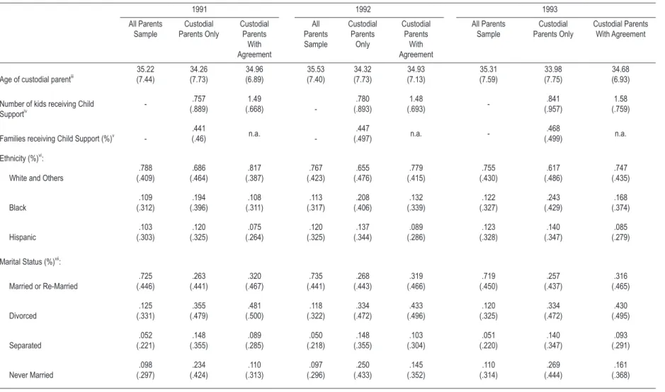
Table 1 presents demographics characteristics for three different sub-samples: All Parents, Custodial Parents Only and Custodial Parents With Agreement. The all parents sample includes families with both parents as well single headed households; custodial parents only is a sub-sam-ple that includes only households characterized by the presence of a children with an absent parent, not mattering if a child support agreement is settled. The final sub-sample is custodial parents with agreement that includes, from the sub-sample custodial parents only, those households where there is some kind of child support agreement.11 This last sub-sample is the main sample for the present analysis.

For all years, the sample that includes all parents has a higher mean age than the sub-sam-ples of single-headed households. The average number of children in families with a child support agreement varies between 1.48 in 1992 and 1.58 in 1993.12 The data also show a small increase in the percentage of families receiving child support (44.1% in 1991 to 46.8% in 1993).

The ethnic profile of child support agreement holders remains fairly constant across sample years. It is interesting to look at the results for minorities, particularly blacks, given their relatively higher incidence of being in single-parent households. (see U.S. Department of Commerce, 1998). For all years, the sample of custodial parents with or without agreement has higher incidence of blacks, compared to the fraction of this ethnicity on the other sub-samples. On average, they repre-sent 11.5% of all parents and 21.5% of all single parents.

More than 70% of individuals with children in the sample are currently married. Among parents with a child support agreement, roughly 45% are currently divorced. When we look at families with child support agreements, we see that never married parents are far more likely to have an agreement than those that are “separated” from their spouse. This fact may indicate that it is easier for a never married person to achieve some kind of child support agreement than for a separated parent. Since the marital status “separated” is usually temporary, this is not a surprising result. Also, separation often is a pre-cursor to divorce, meaning that the relationship between the parents that ended the marriage may make it more difficult to come to a consensus on a child support agreement. The way parents maintain their relationship after the disruption has a funda-mental role in the child support gaps.

8 Conducted in waves 3, 6 or 9, depending on the year. 9 For instance: education, race, marital status, etc.

10 Although linking is one of the best features of the SIPP, it is not possible to link couples after the divorce. The custodial parent provides answers concerning the absent parent. If the couple divorces during the period its household belongs to the SIPP’s sample, both parents will provide answers about their lives, however, the child support questions will be provided only by the custodial one.

11 Notice that neither one of these sub-samples imply a single-headed household. It may be possible that the custodial parent remarried; therefore, he/she is not the only adult on the household.

(5)

R eg in a M ad al o zz o 51 1 Econ. aplic., 11 (4 ): 507-525 , out-dez 200 7

table 1 – demographics characteristics (average) by year and categorized by living arrangements and existence of child supporti,ii

1991 1992 1993

All Parents Sample Custodial Parents Only Custodial Parents With Agreement All Parents Sample Custodial Parents Only Custodial Parents With Agreement All Parents Sample Custodial Parents Only Custodial Parents With Agreement

Age of custodial parentiii

35.22 (7.44) 34.26 (7.73) 34.96 (6.89) 35.53 (7.40) 34.32 (7.73) 34.93 (7.13) 35.31 (7.59) 33.98 (7.75) 34.68 (6.93)

Number of kids receiving Child Supportiv - .757 (.889) 1.49 (.668) -.780 (.893) 1.48 (.693) -.841 (.957) 1.58 (.759)

Families receiving Child Support (%)v

-.441

(.46) n.a.

-.447

(.497) n.a.

-.468

(.499) n.a.

Ethnicity (%)vi:

White and Others

.788 (.409) .686 (.464) .817 (.387) .767 (.423) .655 (.476) .779 (.415) .755 (.430) .617 (.486) .747 (.435) Black .109 (.312) .194 (.396) .108 (.311) .113 (.317) .208 (.406) .132 (.339) .122 (.327) .243 (.429) .168 (.374) Hispanic .103 (.303) .120 (.325) .075 (.264) .120 (.325) .137 (.344) .089 (.286) .123 (.328) .140 (.347) .085 (.279)

Marital Status (%)vii:

Married or Re-Married

(6)

512

New evidence on the determinants of the gap between child support awards and child support receipts

Econ. aplic., 11 (4 ): 507-525 , out-dez 200 7

(continuation table 1)

1991 1992 1993

All Parents Sample Custodial Parents Only Custodial Parents With Agreement All Parents Sample Custodial Parents Only Custodial Parents With Agreement All Parents Sample Custodial Parents Only Custodial Parents With Agreement

Education (%)viii:

Less than High School

.170 (.375) .239 (.426) .161 (.368) .156 (.363) .208 (.405) .124 (.331) .169 (.374) .240 (.427) .172 (.378)

High School Degree

.367 (.482) .385 (.487) .414 (.493) .363 (.481) .385 (.487) .404 (.491) .351 (.477) .367 (.482) .354 (.478) Some college .123 (.328) .138 (.345) .147 (.355) .120 (.325) .141 (.389) .160 (.367) .129 (.335) .144 (.352) .172 (.378) College Degree .340 (.446) .238 (.426) .278 (.448) .361 (.480) .266 (.442) .312 (.464) .351 (.477) .249 (.433) .302 (.459)

Custodial Parent Family Incomeix

3,328 (2,529) 2,235 (1,967) 2,533 (1,892) 3,380 (2,636) 2,335 (2,294) 2,522 (2,195) 3,412 (2,739) 2,211 (2,151) 2,470 (2,240)

Custodial Parent’s Usual Weekly Hours of Work

26.17 (19.81) 26.55 (19.92) 30.34 (18.17) 25.88 (19.88) 26.42 (20.40) 28.49 (18.96) 24.34 (19.86) 23.55 (20.14) 25.12 (19.32)

Custodial Parent’s Usual Weekly Hours of Work (restricted to persons engaged in the Labor Force)

32.00 (17.14) 33.03 (16.72) 35.89 (14.85) 31.23 (17.61) 31.69 (18.25) 32.02 (17.05) 29.65 (17.97) 29.01 (18.47) 28.71 (17.99)

Male (%)x

(7)

R

eg

in

a M

ad

al

o

zz

o

51

3

Econ. aplic.,

11

(4

): 507-525

, out-dez

200

7

(continuation table 1)

1991 1992 1993

All Parents Sample

Custodial Parents Only

Custodial Parents

With Agreement

All Parents Sample

Custodial Parents

Only

Custodial Parents

With Agreement

All Parents Sample

Custodial Parents Only

Custodial Parents

With Agreement

Number of days absent parent use to visit his/her children (during the past 12 months)

- 11.73

(36.52)

25.86

(44.76)

-12.43 (37.96)

28.26

(51.55)

-14.64 (43.85)

33.26 (62.41)

Where does the absent parent live? (%)

Same city/county

-.212 (.409)

.479

(.500)

-.218 (.414)

.488

(.500)

-.224 (.417)

.486 (.500)

Same State (different county)

-.144 (.352)

.315

(.465)

-.129 (.335)

.280

(.450)

-.136 (.342)

.283 (.451)

Different State

-.105 (.307)

.187

(.391)

-.097 (.296)

.170

(.376)

-.105 (.307)

.194 (.396)

Other/ Not Applicable

-.539 (.499)

.019

(.137)

-.527 (.499)

.022

(.148)

-.514 (.500)

.016 (.125)

Unknown - - -

-.029 (.167)

.040

(.196)

-.021 (.144)

.021 (.143)

Number of Observations 5,173 1,616 560 7,173 2,164 772 7,305 2,224 799

(8)

The sample with all parents has a slightly larger number of college graduates than the sub-sam-ples for all years. Single parent households are more likely to be headed by individuals with lower levels of formal education. Family income is on average higher for the all parents sample (more than $3,000) than for the single headed households. It is interesting to notice that families with an agree-ment have higher income than the sample that includes all families with a single head and children (roughly $200 more). Child support agreement compliance may represent an increase in the family income and, in this way, help families to avoid the poverty level. Another possibility is that families with higher income have more resources to fight for a child support agreement or order.13

The descriptive statistics also provide some very interesting, and previously unavailable statis-tics regarding the nature of the child support arrangements. In most agreements, the mother is de-signated as custodial parent;14 very few men are the head of a household with a child and an absent parent. The percentage of men that have custody of a child and have some type of child support agreement is also quite low ranging between 5.8% in 1991 and 3.8% in 1993. However, parents who reach an agreement visit their children more frequently than parents without agreements (approxi-mately 30 days per year against only 13 for parents without an agreement). Previous studies suggest that the more involved a parent is with his/her child’s lives, the more likely the absent parent is to support them financially. (see Robins and Dickinson, 1985).

Finally, the place of non-custodial parent residence appears to be correlated with reaching a child support agreement. More than 70% of the families that achieve an agreement have a non-custodial parent who lives in the same city, county or state. There were incentives to the States to create laws to improve the settlement of agreements, and collection of the amount ordered, between parents living in different States (see Garfinkel, McLanahan and Robins, 1994).15 For the most part, these laws were implemented during the 1990’s, therefore the effects of this new legislation may not be captured by this sample.

3 e

xisteNceaNdmagNitudeofthegap

:

aNempiricaliNvestigatioN

Distinct factors influence child support awards and receipts. As extensively described in Bel-ler and Graham (1993), while some emotional factors16 before and after the separation or divorce influence the willingness to settle a child support agreement, financial conditions of both parents also have some bearing on this decision. Child support receipt is expected to exert great influence over the employment situation of both parent, their income, existence of a new family, State law en-forcement, time spend with children after divorce and custodial parent conditions to look for help on requesting the compliance with the award. My main goal with this investigation is to unders-tand both the custodial parent own characteristics that influence the observance of the agreement, but also the settlement features that may point out the odds of increasing or decreasing the gap between child support orders and receipts.

13 Endogeneity may be playing some rule on these results. The section about multinomial logit model will explore this issue. 14 Over this study, the use of the words “non-resident” and “non-custodial” are interchangeable, since the custody that it is referred

to is the “physical custody”.

15 American society is notoriously recognized by its mobility. The compliance with child support orders decreases when the non-custodial parent moves away from his children. Federal and state laws were created to deal with this problem: the Uniform Interstate Family Support Act was approved by the American Bar Association in 1993 and it is now enacted in all jurisdictions; the Full Faith and Credit for Child Support Orders Act was enacted in 1994; and the Uniform Enforcement of Foreign Judg-ments Act, revised in 1964 and it is enacted in 44 states and DC. See Morgan (1999).

(9)

Econ. aplic., 11(4): 507-525, out-dez 2007 The following analysis is based on the gap between child support orders or agreements, and the self-reported amount received by the custodial parent. The gap variable is defined by:

Gap = Child Support Ordered – Child Support Actually Received (1)

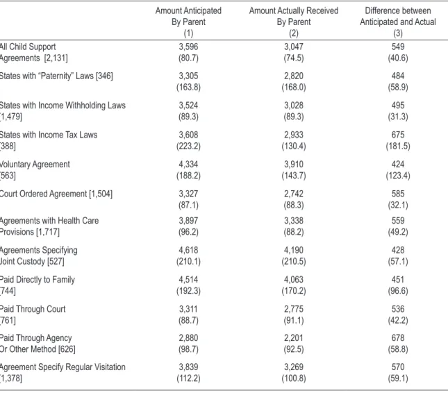
In Table 2, I present descriptive statistics on the gap in child support receipts, as well as the average dollar amount anticipated and the average dollar amount actually received by the custodial parent. For all child support agreements in the sample, the average anticipated amount per year is $3,596 and the average amount actually received is $3,047. Therefore, the average gap for the entire sample of families with a child support award in place is $549. Families holding agreements where the parent’s have joint custody generally have higher anticipated average amounts and lower gaps between expected and actual payments. Anticipated child support awards are also higher for those milies with voluntary agreements and for those families whose payments are made directly to the fa-mily. These facts may be consistent with the hypothesis in which parents that are more involved with their children are more conscious of the financial needs of their kids and responsibilities to them.

table 2 – descriptive statistics (average) for gap 1,2

Amount Anticipated By Parent

(1)

Amount Actually Received By Parent

(2)

Difference between Anticipated and Actual

(3) All Child Support

Agreements [2,131]

3,596 (80.7)

3,047 (74.5)

549 (40.6)

States with “Paternity” Laws [346] 3,305 (163.8)

2,820 (168.0)

484 (58.9)

States with Income Withholding Laws [1,479]

3,524 (89.3)

3,028 (89.3)

495 (31.3)

States with Income Tax Laws [388]

3,608 (223.2)

2,933 (130.4)

675 (181.5)

Voluntary Agreement [563]

4,334 (188.2)

3,910 (143.7)

424 (123.4)

Court Ordered Agreement [1,504] 3,327 (87.1)

2,742 (88.3)

585 (32.1)

Agreements with Health Care Provisions [1,717]

3,897 (96.2)

3,338 (88.2)

559 (49.2)

Agreements Specifying Joint Custody [527]

4,618 (210.1)

4,190 (210.5)

428 (57.1)

Paid Directly to Family [744]

4,514 (192.3)

4,063 (170.2)

451 (96.6)

Paid Through Court [761]

3,311 (88.7)

2,775 (91.1)

536 (42.2)

Paid Through Agency Or Other Method [626]

2,880 (98.7)

2,201 (92.5)

678 (58.8)

Agreement Specify Regular Visitation [1,378]

3,839 (112.2)

3,269 (100.8)

570 (59.1)

(10)

Some specific aspects from the agreement, such as visitation schedule and agency or court being involved in the child support process, are separately analyzed. Agreements with more res-trictions, such as the ones with specific visitation schedule or health care provisions, increase the average gap amount ($570 and $559, respectively). The intermediations of court or agency both in the process of reaching an agreement or receiving the amount settled also contribute to an incre-ase in the default payment. These child support agreement with many restrictions have the worse combination of results possible: lower amounts granted and higher amounts in debt. These results indicate that the relationship between parents closely influences the child support results. When parents do not have to refer to third parts to solve their agreements to make the same agreements to be fulfilled, or when the agreements are very general counting on the responsibility that non-custodial parents feel in relation to their kids, the lower will be the chances that child support will not be paid or that the settled amount is below expectations.

3.1 probit estimation

Equation (4.2) represents the Probit Model:

Probit₍ _{_} ₎

i i

i

gap indicator = α +

∑

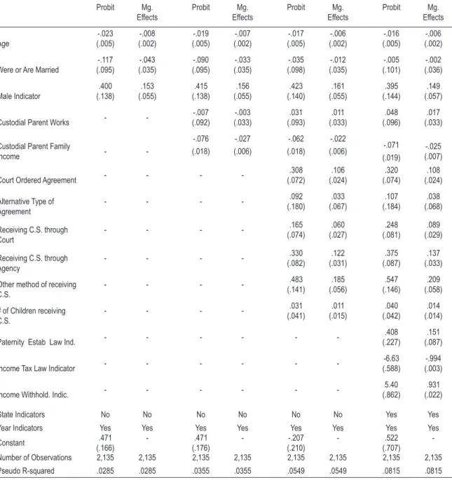
b X +error (2)

where gap indicator is an indicator variable with value 1 if there is a gap between child support orders and receipts, andX_iare the independent variables included in the probit regressions sepa-rately. The demographic characteristics included in X_iinclude the custodial parent’s age, educa-tion level (indicators for high school degree, at least some college and college degree),17 were or are married (indicator variable that assumes value equal 1 if the custodial parent is currently married, divorced or separated, and assumes value equal zero if he/she is never married), ethnicity (indica-tors for Blacks and Hispanic),18 indicator for custodial parent being a male, and year indicators (for 1992 and 1993).19 Table 3 presents the results from this probit equation. As the custodial par-ent gets older, there is a significant decrease in the probability of a gap (-.8%). The higher the level of education and the indicator for the custodial parent being the father have the same influence on the dependent variable (between 6 and 10% for the former and more than 15% for the latter).

In the second column of Table 3, I present results from the same probit regression including demographics and two additional variables. First, I include an indicator variable that equals one if the custodial parent worked at least some period during the two years and half that he/she was included in the sample, and zero otherwise). Second, I include custodial parent family income.20 The inclusion of the custodial parent’s labor force participation dummy and family income changes the significance of the explanatory variables but not their signs. The age of custodial parent still has the effect of decreasing the probability of a gap. However, only custodial parents with at least a college degree have the significant result of decreasing the probability of a default in child support orders (-7.4%). An interesting result is the negative effect that the increase in the custodial parent’s income has on the probability of a gap (-2.7%). This result may be indicating that the richer the

17 Excluded category: less than high school 18 Excluded category: white or others. 19 Excluded category: 1991.

(11)

Econ. aplic., 11(4): 507-525, out-dez 2007 custodial parent, the more resources he/she has available to fight for the right of receiving the child support amount.

table 3 – probability model: probit( _ ) _i _i i

gap indicator = α +

∑

b X +errori,ii

Probit Mg. Effects

Probit Mg. Effects Age -.023 (.005) -.008 (.002) -.019 (.005) -.007 (.002) -.017 (.005) -.006 (.002) -.016 (.005) -.006 (.002)

Were or Are Married

-.117 (.095) -.043 (.035) -.090 (.095) -.033 (.035) -.035 (.098) -.012 (.035) -.005 (.101) -.002 (.036) Male Indicator .400 (.138) .153 (.055) .415 (.138) .156 (.055) .423 (.140) .161 (.055) .395 (.144) .149 (.057)

Custodial Parent Works -

--.007 (.092) -.003 (.033) .031 (.093) .011 (.033) .048 (.096) .017 (.033)

Custodial Parent Family

Income -

--.076 (.018) -.027 (.006) -.062 (.018) -.022 (.006) -.071 (.019) -.025 (.007)

Court Ordered Agreement - - -

-.308 (.072) .106 (.024) .320 (.074) .108 (.024)

Alternative Type of Agreement

- - - - .092

(.180) .033 (.067) .107 (.184) .038 (.068)

Receiving C.S. through Court

- - - - .165

(.074) .060 (.027) .248 (.081) .089 (.029)

Receiving C.S. through Agency

- - - - .330

(.082) .122 (.031) .375 (.087) .137 (.033)

Other method of receiving C.S.

- - - - .483

(.141) .185 (.056) .547 (.146) .209 (.058)

# of Children receiving C.S.

- - - - .031

(.041) .011 (.015) .040 (.042) .014 (.014)

Paternity Estab Law Ind. - - -

-.408 (.227)

.151 (.087)

Income Tax Law Indicator - - -

--6.63 (.588)

-.994 (.003)

Income Withhold. Indic. - - -

-5.40 (.862)

.931 (.022)

State Indicators No No No No No No Yes Yes

Year Indicators Yes Yes Yes Yes Yes Yes Yes Yes

Constant .471 (.166) - .471 (.176) - -.207 (.210) - .522 (.707)

-Number of Observations 2,135 2,135 2,135 2,135 2,135 2,135 2,135 2,135 Pseudo R-squared .0285 .0285 .0355 .0355 .0549 .0549 .0815 .0815

(12)

In the columns 5 and 6 of Table 3, I include characteristics of the child support agreement. Indicator variables for the agreement type (court order or other type of not voluntary agreement),21 how the support ordered amount is received (indicators for through court, through agency or other indirect way to receive child support),22 and number of children included in the child support order were included in the regression. The inclusion of the additional control variables for agreement characteristics has little influence on the significance or magnitude of custodial parent’s age, the indicator for the custodial parent being a male, and custodial parent’s income. However, the child support agreement characteristics are all positive and significant. Agreements settled by court or payments being made indirectly to the custodial parent (i.e. through court, agency or other metho-ds) increase the probability of a gap. The presence of some kind of “intermediary” between parents is positively correlated with the existence of a gap as well. After a marital disruption, there is usu-ally a low level of trust between parents. Non-custodial parent may not believe that his/her money is being used in the best interest of his/her children. The voluntary agreement or direct payments indicate that the relationship between parents is “satisfactory” and, therefore, the trust level betwe-en them is not completely destroyed by the marital disruption. The inclusion of any third part in the child support accord or receipt indicates the lack of reliability between them and, therefore, may positively influence the probability of a failure to pay the agreed or ordered amount.

The final specification for the probit model includes indicator variables for the existence of specific laws to enforce child support and to reduce the number of children without support from the absent parent,23 as well indicator variables for the custodial parent State of residence. The existence of paternity establishment laws or income withholding laws significantly increases the probability that the gap exists. States that have income tax pass-through, on the other hand, have lower probabilities of the existence of a gap.24 These results indicate that specific regulations over child support can have contradictory effects. The plain creation of legislation to improve the well-being of families with single parents does not ensure that this law will be fully implemented as it was planned.25

Changing the basic specification does not significantly inf luence the results. Custodial parent’s age, the father having custody, custodial parent’s family income and agreement specific characteristics are of similar magnitudes and statistically significant for every specification. Ove-rall, results from Table 3 suggest that there is a diminishing probability of a gap in the child sup-port payments the older the custodial parent, the richer his/her family, and if he/she lives in some State where there Income Tax Law in defense of child support agreements/orders exist.

21 Excluded category: voluntary agreement.

22 Excluded category: directly pay to the custodial parent.

23 A very good description of these laws and reasons why they were implemented can be seen in Garfinkel, McLanahan and Robins (1994).

24 The paternity establishment per se does not guarantee that the absent parent will agree or follow a child support order. Income withholding would be a good solution if there was a way to control where the non-custodial parent works, how much he/she earn etc. However, there is no integrated system that can control the labor force movement of non-custodial parent to control movements with the major intention of avoiding child support payments, for example. An ideal system would be very expensive and high-maintenance. Therefore, a law regulating income withholding has the good intention of creating a new support for children with an absent parent, although its effect it is not easily predictable. The Income Tax Law is the simpler way to collect debts from absent parents. For this reason, it is the one with the bigger negative effect in the probability of a gap.

(13)

Econ. aplic., 11(4): 507-525, out-dez 2007 3.2 analysis of the gap’s magnitude

Having studied the determinants of the gap, I now turn my attention to the issue of the size of a child support gap. Different factors can have distinct influences over the magnitude or over the gap’s existence. A simple regression of the gap size on covariates is used:

i i

i

Gap= α +

∑

b X + ε (3)

where X_irepresents the explanatory variables. The custodial parent’s demographic characteristics included are: age, indicators for education degree completed, marital status, ethnicity indicators and gender.26 Custodial parent’s labor force participation and family income are included in the second set of regressions. The income used at this time is relative to earnings from employment and income from assets. I do not use the other sources of income (as, for example, child support receipts, social security, alimony, etc). The third series of regressions include the agreement char-acteristics: type of agreement, how the child support is received, and number of children receiv-ing the child support. The final specification also includes the laws and State indicators. In all regressions, indicators for year in the sample (1992 and 1993, with excluded category 1991) are included.

To account for the potential endogeneity of parental labor supply and the gap between actual and expected payments, I also present evidence from a 2SLS regression where I use the lagged value of custodial parent working as an instrument for current work status. This variable is an indicator that equals 1 if the custodial parent was part of the labor force in the prior months that he/she was included in the sample and zero otherwise.

A good instrument is the one that although is highly correlated with the variable of interest, it is not correlated with the error term, as the instrumented variable is (Gujarati, 1999; Maddala, 1977). The lagged value of the indicator of the working status of the custodial parent has these necessary characteristics, since the past working status has a strong correlation with the current working status and, at the same time, there is no reason to believe that the error term of period t

has correlation with this variable from period t-1. For these reasons, the lagged value of the custo-dial parent working status constitutes a possible instrument for his/her current working status in a 2SLS regression.

The first stage of the system of equations is:

. . _i _i ( . . )

i

Cust Par Works= α +

∑

b X + δLag Cust Par Works + ε (4)

where the indicator variable that specifies if the custodial parent worked last period is the instru-ment for the indicator variable custodial parent currently works. The second stage of the regres-sion is Equation 3, using the estimated values for the instrumented variable from Equation (4).

(14)

Table 4 presents the results for these regressions. Results are reasonable given inclusion of the new variables in the regression. The use of the instrumental variable does not change the signifi-cance or the direction of the result, only the magnitude of the estimated parameters in all cases.

The labor force participation indicator had no effect on the existence of the gap. Table 4 also shows that this variable has a substantial effect in reducing the size of the gap (reduction of $613.25 per year in the gap, using IV approach with the final specification). This result suggests that custo-dial parents that maintain a job increase the level of trust with the absent parent or make him/her realize that his/her kids are really in need of the child support amount. The family income, that decreases the probability of existing a gap, increases its size. It is not a large effect, only $60.23 per year, but it is still significant.

Variables related to the agreement arrangement, as type of agreement or how the amount is received, have the same positive effect over the gap’s amount, increasing its value. The significant estimated parameters are court ordered agreement (increasing by $181 per year the amount in debt), other type of non-voluntary agreement ($455 per year), receiving the child support by indirect me-thods that not through court or agency ($468), and number of children with child support order ($157). Neither one of the laws related to child support enforcement have significant effect on the gap’s magnitude.

In general, results from Table 4 show that, while some demographics characteristics of cus-todial parent are important for the existence of the gap, they have no significant effect on its size. The most important variables for the definition of size gap are the custodial parent’s labor force profile and income, and the agreement characteristics. This result suggests that the relationship among parents is the base for the fulfillment of the agreement. Courts and agency work on hel-ping men and women that stroke with the responsibility of sustaining children without their other parent, while the laws make the effort of serving the interest of single-parent homes too. However, their work is vastely facilitated when absent parent gets more conscious of his/her obligation with the previous family. This receptiveness leads to an improvement of the bond both with his/her ex-partner as well with his/her children.

table 4 – regressions: gap = i i i

X

α +

∑

b + ε

Instrumental Variable: Lag( Custodial Parent Works)

Baseline Regression

Incorporating Labor Force Characteristics

Incorporating Agreement Characteristics

Incorporating Enforcement and Time Effects

(OLS) (OLS) (IV) (OLS) (IV) (OLS) (IV)

Age

-3.45 (6.39)

-5.31 (6.50)

-5.08 (6.51)

-3.74 (6.53)

-3.55 (6.54)

-1.35 (6.52)

-1.11 (6.53)

High School Indicator

-171.24 (124.76)

-114.96 (126.19)

-64.81 (127.46)

-84.96 (126.45)

-42.49 (127.56)

-94.64 (127.36)

-58.53 (128.47)

Some College Indicator

115.07 (147.47)

149.17 (149.29)

195.86 (150.31)

175.59 (149.47)

216.61 (150.41)

176.54 (150.17)

210.48 (151.06)

College Degree Indicator

-201.97 (132.67)

-171.20 (137.27)

-114.02 (138.76)

-146.89 (137.91)

-97.75 (139.25)

-159.52 (138.18)

-118.85 (139.46)

Were or Are Married

85.10 (138.05)

91.03 (138.00)

105.98 (138.30)

72.77 (140.85)

87.08 (141.13)

61.29 (141.93)

(15)

Econ. aplic., 11(4): 507-525, out-dez 2007 Baseline

Regression

Incorporating Labor Force Characteristics

Incorporating Agreement Characteristics

Incorporating Enforcement and Time Effects

(OLS) (OLS) (IV) (OLS) (IV) (OLS) (IV)

Black Indicator .545 (135.84) 12.34 (136.84) -2.45 (137.13) -24.25 (137.31) -37.87 (137.57) -70.83 (144.14) -79.64 (144.33) Hispanic Indicator 127.16 (152.14) 123.42 (152.35) 105.18 (152.70) 111.01 (152.08) 94.88 (152.39) 70.89 (158.12) 61.03 (158.32) Male Indicator 44.66 (199.50) 64.74 (199.00) 83.08 (199.39) 62.56 (198.59) 78.99 (198.93) 30.06 (199.58) 42.12 (199.83)

Custodial Parent Works

--479.04 (132.17) -816.20 (172.78) -428.47 (133.01) -738.09 (174.80) -352.78 (133.52) -613.25 (176.21)

Custodial Parent Family Income - 53.36 (23.82) 62.25 (24.04) 64.78 (24.01) 71.88 (24.18) 54.03 (24.18) 60.23 (24.36) Court Ordered Agreement

- - - 163.58

(96.91) 160.43 (97.04) 183.45 (97.05) 180.62 (97.15)

Alternative Type of Agreement

- - - 370.71

(247.61) 376.94 (247.94) 450.03 (248.09) 455.02 (248.32)

Receiving C.S. through Court

- - - 60.59

(100.9) 61.84 (100.99) 176.26 (108.79) 174.27 (108.90)

Receiving C.S. through Agency

- - - 144.84

(114.27) 127.62 (114.59) 185.00 (119.03) 168.68 (119.33)

Other method of receiving C.S.

- - - 411.72

(202.39) 411.67 (202.65) 468.23 (202.88) 468.29 (203.07)

Number of Children receiving C.S.

- - - 156.93

(57.93) 142.91 (58.23) 168.39 (57.87) 157.27 (58.13) Paternity Establishment Law Ind.

- - - 270.23

(298.89)

293.49 (299.34)

Income Tax Law Indicator - - - -

--455.50 (806.57) -1162.16 (1356.10) Income Withholding Indicator

- - - 219.59

(952.35)

220.22 (953.22)

State Indicators No No No No No Yes Yes

Year Indicators Yes Yes Yes Yes Yes Yes Yes

Constant 566.25 (238.11) 868.28 (251.03) 1,077 (260.62) 297.96 (296.61) 521.64 (308.05) 192.69 (1251) 1083.97 (975.26) Number of Observations 2,135 2,135 2,135 2,135 2,135 2,135 2,135

Adjusted R-squared .004 .010 .007 .016 .013 .038 .036

Note: Standard Errors are in parentheses and the same notes from tables 1 and 3.

(16)

Econ. aplic., 11(4): 507-525, out-dez 2007 3.3 multinomial logit analysis

As shown in the previous regressions, agreement type is a significant factor in the existence and the size of the gap. However, agreement type could be an endogenous variableto the parents’ characteristics,27 since its choice may reflect the level of animosity between the parents. When the ex-couple has difficulties in reaching agreements, it is more likely that they will have problems following the guidelines predetermined by this agreement, therefore the importance of including the dummies for the previous regressions. The multinomial logit analysis is used to illustrate the mechanism that may underlie the resulting agreement type.

In the present study, an agreement can be reached in three ways: A₁ = voluntarily,

A₂ = court ordered, or A₃ = alternative agreement.

In order to predict the determinants of agreement type, I use the custodial parent’s characte-ristics, including age, schooling, race, labor force participation, and number of children involved with child support. The main goal of this exercise is to observe how custodial parent’s characteris-tics increase or decrease the probability of obtaining one of the three particular types of agreement the basic model of agreement type definition is28

Prob (Ai = j) =

'

j i

k i

X

k e

e

b

=

∑

3

1

(5)

where X_iis the vector of custodial parent’ socioeconomic characteristics and bis the vector that defines the probabilities of each type of agreement being reached. Presented this way, this model is indeterminate. The solution for the model indeterminacy is normalization, where one of the categories of agreement is set equal to zero. I choose the category “voluntary agreement” to be zero and, by this, it will be the base category. All the results from the multinomial estimation are interpreted by comparison with the base category, voluntary agreement.

After the normalization, the intuitive way to look at equation 5 is

'

ln ij _j _i

i P

X P

 

= b

 

 1

(6)

Equation 6 shows that the logarithm of the probability that some custodial parent reaches a specific type of agreement is a linear function of the custodial parent’s characteristics. Although this equation is very simple, its interpretation is not trivial. It is not possible to interpret the estima-ted bj coefficient as the outcome from the j agreement type. Every marginal effect will include the entire b vector. Therefore, the simpler and more useful way to interpret the estimated coefficient will be by comparison with the chosen base category.

27 Notice that the type of agreement is not endogenous to the existence neither the magnitude of the gap between child support awards and receipts.

(17)

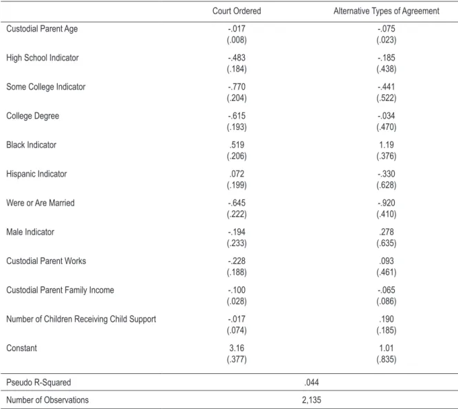
Econ. aplic., 11(4): 507-525, out-dez 2007 The probability of voluntary agreement is higher when both the coefficients for the court ordered category and other types of agreement are negative and significant. As Table 5 shows, this happens in three cases: when the custodial parent is older, when he/she is not single, and when he/she is not black or Hispanic. Table 5 also shows that there are two cases where it lowers the pro-bability of a court order settlement:29 when the custodial parent has more years of education, and when his/her family income is higher.

table 5 – maximum-likelihood multinomial logit i,ii: prob (a_i = j) =

'

j i

k i

X

k e

e

b

=

∑

3

1 omitted category: voluntary agreement

Court Ordered Alternative Types of Agreement

Custodial Parent Age -.017

(.008)

-.075 (.023)

High School Indicator -.483

(.184)

-.185 (.438)

Some College Indicator -.770

(.204)

-.441 (.522)

College Degree -.615

(.193)

-.034 (.470)

Black Indicator .519

(.206)

1.19 (.376)

Hispanic Indicator .072

(.199)

-.330 (.628)

Were or Are Married -.645

(.222)

-.920 (.410)

Male Indicator -.194

(.233)

.278 (.635)

Custodial Parent Works -.228

(.188)

.093 (.461)

Custodial Parent Family Income -.100 (.028)

-.065 (.086)

Number of Children Receiving Child Support -.017 (.074)

.190 (.185)

Constant 3.16

(.377)

1.01 (.835)

Pseudo R-Squared .044

Number of Observations 2,135

Notes: i) Results from the Maximum-Likelihood Multinomial Logit should be compared to the omitted category, Voluntary Agreement. ii) Standard Errors are in parentheses.

(18)

The multinomial logit model clarifies some trends behind the personal attributes of custodial parents that define the type of agreement that can be reached. However, it is not enough evidence to accept or reject the hypothesis of endogeneity between the gap and types of agreement.

4 c

oNclusioN

The importance of child support to a society where there is an increasing number of single-parent families and where a great proportion of children are expected to live some part of their childhood with only one parent (U.S. Census Bureau, 1999; and Robins and Dickinson, 1985) is not disputable. Federal and state governments acted to improve the situation of these families and children that have a larger probability of becoming poor (Garfinkel, McLanahan and Robins, 1994). The implications of these legislative changes and the effects that custodial and non-custodial parents main characteristics had over the child support orders and their collection were separately studied by different authors (Beller and Graham, 1993; Sonestein and Calhoun, 1990; and Veum, 1992).

This study analyzes both the probability of a gap between child support orders and child support receipts, as well the characteristics from the custodial parent and the agreement that may influence the size of this gap. While there is a decreasing probability of the gap’s existence, the older the custodial parent, the wealthier is his/her family, and the closer the residence of the non-custodial parent, these variables do not have the same influence over the size of the gap. For the magnitude of the difference between amounts ordered and received, the most important features are the labor force participation of custodial parent and the agreement’s characteristics.30 Custodial parents that are involved in the labor market signal to their former partner that they are doing their part in trying to support children and, by this, the smaller the gap between child support orders and receipts attributed to them. The agreement characteristics results support the idea that parents with a good relationship after their marital disruption do not need an intermediate either for the child support order or its collection. This better connection between parents improves the odds of the child support being completely paid and, whenever this payment is partial, the difference be-tween the order and the amount actually received is smaller than when compared to child support orders intermediated by third parts (e.g., courts or agencies).

The improvement in the enforcement of child support laws and the creation of institutions that help custodial parents to collect the money to sustain children that no longer live with both pa-rents are well intended and have positive effects for child support collection. The impact that these laws and institutions have over the child support gaps is not within the scope of this paper. Results presented here corroborate the idea that the association of tougher laws concerning fulfillment of child support and stronger links between parents. Therefore, a good relationship after they broke up improves the likelihood of full collection of child support and/or lower debts to be collected.

r

efereNces

BELLER, A. H.; GRAHAM, J. W. Small change: the economics of child support Yale University, USA,

1993. book.

(19)

GARFINKEL, I.; MCLANAHAN, S. S. ROBINS, P. K. child Support; child Well-Being. The Urban

Institute Press, Washington, D.C., 1994. book.

GREENE, W. H. Econometric analysis. 3th ed. New Jersey, USA: Prentice Hall, 1997

GUJARATI, D. Essentials of Econometrics. 2th ed. USA: Irwin/McGraw-Hill, 1999.

JOHNSON, JOHN H. Revisiting the impact of tougher child support enforcement. In: CSWEP Session on

the Economics of Marriage; Family at the 2001 ASSA Meetings in New Orleans, 2001.

MADDALA, G. Econometrics. USA: McGraw-Hill, 1977.

MCLANAHAN, S.; SANDEFUR, G. Growing up with a single parent: what husrts, what helps Cambridge;

London: Harvard University Press book, 1994.

MORGAN, L. interstate enforcement of support: a short primer on federal; uniform law. National Legal

Research Group, 1999.

NERLOVE, M.; PRESS, S. univariate; multivariate log-linear; logistic models. Santa Monica:

RAND-R1306-EDA/NIH, 1973.

NIxON, L. The effect of child support enforcement on marital dissolution. Journal of Human Resources,

v. 32, n. 1, p. 159-81, 1994.

PETERSON, J.; NORD, C. The regular receipt of child support: a multi-step process. U. S. Department of

Commerce, Bureau of the Census, 1989. (Working Paper n. 102).

ROBINS, P. K; DICKINSON, K. Child support; welfare dependence: a multinomial logit analysis.

De-mography, v. 22, iss. 3, p. 367-380, 1985.

SONESTEIN, F. L.; CALHOUN, C. A. Determinants of child support: a pilot survey of absent parents.

contemporary policy issues, v. 8, Jan., p. 75-109, 1990.

SORENSEN, E.; HALPERN, A. child support enforcement: how well is it doing? Urban Institute, 1999.

(Discussion Paper 99-11).

THEIL, H. A Multinomial extension of the linear logit model. international Economic Review, v. 10, p.

251-60, 1969.

U. S. CENSUS BUREAU. annual demographic survey: march supplement. Internet Release: Oct. 3, 1997.

________. living arrangements of children under 18 years old. Internet Release: Jan. 7, 1999.

________. Statistical abstract of the united States: 2000. 2000.

U. S. DEPARTMENT OF COMMERCE, BUREAU OF CENSUS. Marital status; livinig arrangements:

march 1996. Current Population Reports, Series P20-496, Mar. 1998.

VEUM, J. R. Interrelation of child support, visitation, hours of work. Monthly labor Review, p. 40-47,

Jun. 1992.

WEESIE, JEROEN. Sg 121: seemingly unrelated estimation; the cluster-adjusted sandwich estimator. Stata