THE TIME-(IN)VARIANT INTERPLAY OF
GOVERNMENT SPENDING AND PRIVATE
CONSUMPTION IN BRAZIL
Diego Ferreira*
Abstract
This paper analyzes the relationship between government spending and private consumption in Brazil through an application of a VAR with time-varying parameters and stochastic volatility, estimated with Bayesian simulation over the 1996:Q1–2014:Q2 period. The findings reveal that fiscal policy is indeed effective in stimulating GDP and private consump-tion, which characterizes the presence of positive Keynesian multipliers. However, these positive effects are only sustained on the short-run. Also, stochastic volatility seems to have decreased from 2000 onwards, suggest-ing that Brazil has steadily improved its macroeconomic stability after the adoption of the inflation-targeting framework and the Fiscal Responsibil-ity Law.
Keywords:Government Spending; Private Consumption; TVP-VAR.
Resumo
O presente estudo analisa a relação entre gasto público e consumo pri-vado no Brasil através de um modelo VAR com parâmetros variantes no tempo e volatilidade estocástica, estimado com simulação bayesiana para o período 1996:T1–2014:T2. Nossos resultados revelam que a política fis-cal é de fato efetiva para estimular o PIB e o consumo privado, caracteri-zando a presenção de multiplicadores keynesianos positivos. Porém, tais efeitos positivos apenas são sustentados no curtíssimo-prazo. Além disso, a volatilidade estocástica se reduziu a partir de 2000, revelando um ambi-ente macroeconômico mais sólido após a adoção do regime de metas para inflação e da Lei de Responsabilidade Fiscal.
Palavras-chave:Gasto Público; Consumo Privado; TVP-VAR. JEL classification:E62, E32, C32, D78
DOI:http://dx.doi.org/10.1590/1413-8050/ea125573
*Federal University of Paraná, UFPR, Brazil. E-mail: [email protected]
1 Introduction
The depth of the recent global recession has rekindled the debate on the role of discretionary fiscal policy. In order to mitigate the potential economic down-turn and ensure the resilience of the financial system, governments around the world have designed unprecedented fiscal stimulus packages. However, due to controversial predictions of neoclassical and Keynesian oriented mo-dels, there remains no macroeconomic consensus on the interplay of govern-ment spending shocks and private consumption.
Since the seminal paper by Barro (1974), which introduced the concept of
Ricardian Equivalence, there has been a resurgence in the debate on the
pos-sible non-Keynesian effects of fiscal policies. By embodying this feature, the
future tax burden of present fiscal stimulus restrains the Keynesian effects
on private consumption (Mankiw & Summers 1984, Blanchard 1985). Moreo-ver, models of neoclassical tradition argue that the intertemporal substitution effects on labor supply are not strong enough to offset the negative wealth
ef-fects driven by an increase on government spending (see e.g. Barro & King (1984) and Baxter & King (1993)).
By amending the Real Business Cycles (RBC) framework to allow for mo-nopolistic competition and nominal rigidities, macroeconomic modeling de-parted from price flexibility in order to achieve short-run non-neutrality of money. Regarding the effectiveness of fiscal policy to stimulate private
con-sumption, these so called New Keynesian models formerly presented unexpec-ted non-Keynesian responses (Smets & Wouters 2003, Linnemann & Schabert 2003, Cogan et al. 2010, Cwik & Wieland 2011).
However, empirical evidences - mainly based on vector autoregressions (VAR) — depicted another conclusion. For instance, with a structural VAR approach, Blanchard & Perotti (2002) obtained positive public spending mul-tipliers for output and private consumption with US postwar data. Using the same estimation technique as the latter, Perotti (2002) verified positive mul-tipliers for United Kingdom, Germany, Canada and Australia, despite their downward trend over time. Furthermore, many other papers have used simi-lar approaches1, including Fatás & Mihov (2001), Ramey (2008), Mountford & Uhlig (2009), Fisher & Peters (2009) and Ilzetzki et al. (2013).
Following Mankiw (2000)2, Galí et al. (2007) proposed a new feature to
the New Keynesian framework in an attempt to counter these theoretical and empirical divergences. By introducing the coexistence of non-Ricardian (
rule-of-thumb) and intertemporal optimizing households, the authors generated
standard Keynesian effects of government spending expansions for the US
economy, arguing that the usual negative wealth effect was damped. The
stu-dies of Linnemann (2006), Ravn et al. (2006) and Forni et al. (2009) supported the latter results. On the other hand, one should not generalize these findings. Coenen & Straub (2005) showed that the presence of positive public spen-ding multipliers for private consumption is directly related to the share of
1Despite the choice of a structural VAR framework, the identification restrictions imposed
differ. For instance, Fatás & Mihov (2001) applied the standard recursive approach (Cholesky
decomposition) introduced by Sims (1980), while Mountford & Uhlig (2009) used the sign-restrictions scheme. Besides, Blanchard & Perotti (2002) and Perotti (2002) assigned structural restrictions based on fiscal institutional information.
2Mankiw (2000) pointed out that non-Ricardian households were a crucial element in order
non-Ricardian households in the population. Moreover, Ratto et al. (2009) and Furceri & Mourougane (2010) highlighted labor market adjustment costs and financial market stress as restrictions to the expected Keynesian effects of
fiscal policies, respectively.
Regarding the Brazilian economy, empirical evidences are ambiguous as well as scarce. Silva & Cândido Júnior (2009) evaluated the 1970–2002 pe-riod through an application of cointegration in VAR models, concluding that government spending crowds out private consumption in the long-run even though positive government spending shocks initially increase private con-sumption. Thus, these results advocate against the effectiveness of
discretio-nary fiscal policy as a countercyclical measure since its positive effects would
be restricted to the short-run. Silva & Portugal (2010) corroborated the latter non-Keynesian effects of fiscal policy for Brazil through a DSGE model with
non-Ricardian and intertemporal optimizing households. The authors argued that the share of Brazilian liquidity constrained households is rather low (ne-arly 10%), hence unable to offset the negative wealth effect from a government
spending shock.
On the other hand, Mendonça et al. (2009) presented crowding in effects
of government spending on private consumption over a 1995–2007 sample. Furthermore, while evaluating the period after the introduction of the Real Plan (1994–2012) with VAR models, Peres (2012) also identified standard positive Keynesian responses for the interplay of government spending and private consumption. By analyzing developed and developing economies th-rough a panel error-correction model both uniequational (P-ECM) and multi-equational (P-VECM) for 48 countries, Soave & Sakurai (2012) also presented empirical evidences of crowding in effects on consumption in the long-run,
especially for the developing ones (including Brazil).
However, the fiscal transmission channels are likely subject to changes over time. Empirical support for the latter proposition comes, for instance, from the study of Kirchner et al. (2010), which showed that the short run government spending multipliers in the Euro area increased from the early 1980s until the late 1980s, but presented a decreasing trend thereafter. Mo-reover, Pereira & Lopes (2010) argue that fiscal policy has lost its capacity to stimulate output in the US economy from 1965 to 2009, despite positive multipliers. Yet, Brazilian literature has struggled so far to provide results accounting for potential time heterogeneity patterns. To the best of my kno-wledge, the present paper is the first attempt of evaluating the time-varying interplay of government spending and private consumption for Brazil.
Besides the reforms implemented by the Real Plan in 1994 and the adop-tion of a floating exchange rate regime along with an inflaadop-tion-targeting fra-mework in 1999, the establishment of the Brazilian Fiscal Responsibility Law in 2000 as well as the presence of fiscal stimulus packages in face of the 2008 financial crisis might have contributed to shifts in the Brazilian fiscal dyna-mics. Additionally, given the outburst of consumer credit growth rates in Brazil since 2005 (Freitas 2009, Hansen & Sulla 2013), this recent transition of the share of non-Ricardian households might have also affected the eff
ecti-veness of fiscal policy throughout the sample3.
3While assessing these effects in developed and developing countries under the hypothesis
In light of the facts formerly mentioned, a four-variable time-varying pa-rameter (TVP) VAR model is estimated for Brazil, following closely Kirchner et al. (2010). The model includes government spending, GDP, short-term in-terest rate and private consumption over the period 1996:Q1-2014:Q2. Since structural changes cannot be easily identified prior to estimation and might also be part of a long process, the TVP-VAR stands as a method capable of cap-turing these time-varying effects in a robust and flexible manner (Nakajima
2011). By allowing for time-variation in the autoregressive parameters and stochastic volatility, it is possible to deal with potential non-linearity during estimation. As the parameters follow a first-order random walk process, the method is able to capture both temporary and permanent shifts. In compa-rison to Markov-switching models, the random walk specification allows for smooth shifts in contrast to discrete breaks, being more suitable for descri-bing changes in private sector behavior or the learning dynamics of both pri-vate agents and policy makers (Primiceri 2005). Moreover, given the potential effects of exogenous shocks over the volatility of macroeconomic aggregates,
ignoring conditional heteroskedasticity might lead to spurious movements in time-varying variables and inaccurate inference (Hamilton 2010). Thus, the stochastic volatility specification is included to take this issue into account.
The findings reveal that fiscal policy is indeed effective in stimulating GDP
and private consumption, which characterizes the presence of positive Keyne-sian multipliers. Even though the overall response of the variables to a po-sitive government spending shock seems to be rather similar throughout the sample period, the time-varying techniques indicate some increasing persis-tence of its effectiveness. Besides, the stochastic volatility decrease from 2000
onwards suggests that Brazil has steadily improved its macroeconomic sta-bility after the adoption of the inflation-targeting framework and the Fiscal Responsibility Law.
The remainder of this paper is organized as follows. Section 2 introduces the vector autoregression (VAR) models and how time-varyingfeatures were implemented on these models, in order to capture potential changes on macro-economic behavior over time. Furthermore, it describes the data set and the Bayesian estimation procedure. Section 3 presents the empirical results, high-lighting the effectiveness of government spending shocks. A time-invariant
comparison through an application of a Bayesian VAR as well as a prior sensi-tivity analysis are also performed. Finally, section 4 presents the conclusion.
2 Econometric Methodology
2.1 Time-Varying Parameter (TVP) Bayesian Vector Autoregression Model with Stochastic Volatility (SV)
Since Sims (1980), the vector autoregression (VAR) model has played a pro-minent role on macroeconometric analysis. Considered a flexible and easy tool for dealing with multivariate time series, it generally consists in a
multi-interaction of government spending and private consumption. Yet, Tagkalakis (2008) emphasi-zed that government spending multipliers on private consumption and real output depend on
the stage of the business cycle, granted that recessions tend to raise the effectiveness of
equation system describing the economic dynamics. A basic structural VAR model can be defined as:
Ayt=F1yt−1+· · ·+Fsyt−s+ut, t=s+ 1, . . . , n, (1)
whereytis ak×1 vector of observed variables;Ais ak×kmatrix of contempora-neous relationships;F1, . . . , Fnis ak×kmatrix of coefficients; andut∼N(0,ΣΣ) is ak×1 structural shock vector, with:
Σ=
σ1 0 · · · 0
0 . .. ... ...
..
. . .. ... 0
0 · · · 0 σk
(2)
However, one cannot directly estimate Equation (1) since its structure al-lowsAandF to show an infinite set of different values with exactly the same
probability distribution, hence data alone cannot provide the true values of
AandF. Therefore, by assuming that the simultaneous relations of the struc-tural shock are identified by a recursive approach, which imposes Ato be a lower-triangular matrix with the diagonal elements equal to one, the Equation (1) can be re-specified as a reduced form VAR model:
yt=B1yt−1+· · ·+Bsyt−s+A−1Σεt, εt∼N(0, Ik), (3)
whereBi≡A−1Fi, fori= 1, . . . , sand:
A=
1 0 · · · 0
a21 . .. . .. ...
..
. . .. . .. 0
ak1 · · · ak,k−1 1
(4)
DefiningBas a stacked row ofB1, . . . , Bs andXt≡Ik⊗(y
′
t−1, . . . , y
′
t−s), where
⊗represents the Kronecker product, the reduced form of Equation (3) can be rewritten as:
yt=Xtβ+A−1Σεt, (5)
Although the parameters β, A and Σ in Equation (5) are time-invariant,
these can re-specified to account for time-varying analysis as well. Following Primiceri (2005) and Nakajima (2011), one can rewrite Equation (5) as:
yt=Xtβt+At−1Σtεt, t=s+ 1, . . . , n, (6)
whose parameters are all time-varying4. Leta
t = (a21, a31, a32, a41, . . . , ak,k−1)
′
be a stacked vector of the lower-triangular elements inAtandht= (h1t, . . . , hkt)
′
4As discussed in Nakajima (2011), time-varying intercepts can also be incorporated in
TVP-VAR models by definingXt≡Ik⊗(1, y
′ t−1, . . . , y
withhjt= logσjt2, forj= 1, . . . , k andt=s+ 1, . . . , n, the parameters in Equation (6) are assumed to follow drift less random walk processes5, given by:
βt+1=βt+uβt, at+1=at+uat, ht+1=ht+uht, (7)
εt
uβt
uat
uht ∼N
0,
I 0 0 0
0 Σβ 0 0
0 0 Σa 0
0 0 0 Σh
, (8)
for t=s+ 1, . . . , n, whereI is the identity matrix of k dimensions, whileΣ
β,
Σa and Σh are positive definite matrices, whose elements are usually called
the hyperparameters. As in Nakajima (2011), shocks are assumed uncorrela-ted among the time-varying parameters and the covariance matricesΣβ,Σa
and Σh are assumed to be diagonal6. Moreover, βs+1 ∼N(µβ
0,Σβ0), as+1 ∼
N(µa0,Σa0) and hs+1 ∼ N(µh0,Σh0), which are the initial states of the
time-varying parameters.
Since TVP-VAR models with stochastic volatility are non-linear non-Gaussian state-space representations, the Maximum Likelihood (ML) approach cannot provide reliable estimates for the parameters. Also, allowing for time-variation in the parameters of a VAR framework as well as in the error covariance ma-trix causes serious concerns about over-parameterization (Koop & Korobilis 2010). Therefore, the Bayesian approach using the Markov chain Monte Carlo (MCMC) method is by now fairly standard in dealing with this class of models (e.g. Primiceri (2005) and Nakajima (2011)).
By splitting up the original problem into a number of smaller steps, the Bayesian inference is able to deal with high-dimensional parameter space and potential non-linearities in the likelihood function. Under the assumption of a certain prior probability density, the MCMC algorithm is able to generate the joint posterior distribution of the parameters, given as:
p(θ|y) =R p(θ)L(y|θ) θp(θ)L(y|θ)dθ
∝p(θ)L(y|θ) (9)
wherey={yt}nt=1;θ=
n
β, a, h,Σβ,Σa,Σho;p(θ) is the prior density distribution;
p(θ|y) is the posterior density distribution; andL(y|θ) is the likelihood
func-tion. In other words, given y, the MCMC simulation draws samples from
p(θ|y) in order to achieve the values ofθ. This drawing process can be descri-bed by the following MCMC algorithm7:
1. Initializeθ;
2. Sampleβ|a, h,Σβ andy;
3. SampleΣ
β|β;
5One should note that the volatility states (h
t) evolve as geometric random walks, hence
depicting a TVP-VAR model with stochastic volatility (SV) as in Primiceri (2005). By including the time-varying stochastic volatility to the VAR estimation, one can prevent potential biases in
the covariance matrix for the disturbances and in the autoregressive coefficients because of the
misspecification of the dynamics of the parameters (Nakajima et al. 2009).
6Nakajima (2011) argues that the diagonal assumption forΣβ,ΣaandΣh does not affect
sensitively the results when compared to the non-diagonal assumption.
4. Samplea|β, h,Σ
a andy; 5. SampleΣa|a;
6. Sampleh|β, a,Σ
handy; 7. SampleΣh|h;
8. Return to 2.
Regarding the choice of priors, this paper sets rather diffuse and
uninfor-mative priors, following the study of Nakajima (2011)8:
(Σβ)−2
i ∼G(25,0.01I), (Σa)−i2∼G(4,0.01), (Σh)i−2∼G(4,0.01) (10)
where (Σβ)−2
i , (Σa)
−2
i and (Σh)
−2
i represents thei-th diagonal element of the matrices and G is the Gamma distribution. In addition, flat priors were set to the initial states of the time-varying parameters, such thatµβ0=µa0=µh0= 0
and Σβ
0 =Σa0 =Σh0 = 10×I. Also, following the Akaike information
crite-rion (AIC) and the Schwarz information critecrite-rion (SBC), applied to a time-invariant VAR, the TVP-VAR is estimated based on two lags9.
As for the identification procedure, establishing the simultaneous relati-ons of the structural shocks is not a trivial task. Following Kirchner et al. (2010), this paper resorts to a recursive identification framework for fiscal po-licy10. Based on the seminal work of Blanchard & Perotti (2002), the contem-poraneous interactions between government spending and the macroecono-mic environment can be completely assigned to the working of automatic sta-bilizers, hence discretionary fiscal policy would not respond within the same quarter to macroeconomic shocks due to political decision-lags. Government spending shocks are identified as predetermined in a system with output, in-terest rate and private consumption, being ordered first in a Cholesky-type variance-covariance decomposition scheme11. One should notice that the
lat-ter identification procedure is commonly adopted by the lilat-terature on fiscal policy (Perotti 2002, 2007, Caldara & Kamps 2008, Ramey 2008, Kirchner et al. 2010).
2.2 Data Description
In order to evaluate the time-variation and the potential effects of Brazilian
fiscal policy, we use quarterly data from 1996:Q1 until 2014:Q2, which cor-responds to the period after the introduction of the Real Plan (1994) and the adoption of the inflation-targeting regime (1999). Furthermore, by using quar-terly data, we exclude the possibility of fiscal policy discretionary response to macroeconomic shocks within the quarter. The VAR specification includes
8In order to evaluate the robustness of the chosen priors, a sensitivity analysis discussion is
carried out in Subsection 3.3.
9These results are available upon request from the author.
10Even though the TVP-VAR models allow for time-varying features, the identification scheme
is assumed to be time-invariant over the sample.
11Although the present identification scheme can be arguable (as is often the case in a
Cho-lesky ordering), the data frequency grants a sufficient degree of flexibility. Moreover, for the
purposes of identifying just the dynamic effects of government spending shocks, it is not
government spending (measured as government final consumption expendi-ture)12, private consumption (measured as private final consumption expendi-ture), GDP (measured as factor prices) and short-term interest rate (measured as Brazilian Central Bank’s overnight call rate). The time series were downlo-aded from the Brazilian Institute of Geography and Statistics (IBGE) and the Brazilian Central Bank (BCB).
Government spending, private consumption and GDP were first realized by the Extended National Consumer Price Index (IPCA), whose base is 1996:Q1, and then seasonally adjusted, applying the X-12-ARIMA method. Moreover, the latter data series enter the analysis in the form of their respective realper
capita13 values. The short-term interest rate is expressed in nominal, annual
terms.
Figure 1 and Figure 2 present the Brazilian data used in the model speci-fication. In general, the time series present contrasting patterns, which can be seen as a first indication that a time-varying parameter model might be the suitable choice. For instance, one can identify two seemingly distinctive sub-sample periods: from 1996 to the end of 2002, and from 2003 onwards.
800 900 1,000 1,100 1,200 1,300 1,400 1,500
9697 98 9900 01 0203 04 0506 07 0809 10 1112 13 14
Gross Domestic Product (R$)
200 240 280 320 360 400
96 97 9899 00 0102 03 0405 06 0708 09 1011 12 13 14
Government Spending (R$)
600 700 800 900 1,000 1,100 1,200
9697 98 9900 01 0203 04 0506 07 0809 1011 12 13 14
Private Consumption (R$)
0 10 20 30 40
96 97 9899 00 0102 03 0405 06 0708 09 1011 12 13 14
Short-Term Interest Rate (%)
Notes: Shaded area corresponds to Luiz Inácio “Lula” da Silva 1st and 2nd terms as president; government spending (GS), private consumption (PC) and GDP are all expressed
in realper capitaterms and seasonally adjusted; short-term interest rate is measured in
nominal, annual terms.
Sources: Brazilian Institute of Geography and Statistics (IBGE) and Brazilian Central Bank (BCB).
Figura 1: Brazilian Data (1996:Q1–2014:Q2)
Based on standard unit root tests, namely, the Augmented Dickey-Fuller (ADF) (Dickey & Fuller 1981) test, the Phillips-Perron (PP) (?) test and the Kwiatkowski, Phillips, Schmidt, and Shin (KPSS) (Kwiatkowski et al. 1992) test, the data series were found to be non-stationary in general, hence conver-ted to their corresponding growth rate14. The test statistics and the specifica-tion for the deterministic terms are presented in Table (1).
12The government final consumption expenditure time series sums up expenditures from
cen-tral administration agencies and decencen-tralized entities (independent agencies, foundations and funds) at federal, state and municipal spheres. It also considers parastatal entities, such as the S System and Federal Councils.
-12 -8 -4 0 4 8 12 16
1996 1998 2000 2002 2004 2006 2008 2010 2012 2014
Short-Term Interest Rate - First Difference (%) -4
-2 0 2 4 6
1996 1998 2000 2002 2004 2006 2008 2010 2012 2014 Gross Domestic Product - Growth Rate (%)
-10 -5 0 5 10 15
1996 1998 2000 2002 2004 2006 2008 2010 2012 2014 Government Spending - Growth Rate (%)
-6 -4 -2 0 2 4 6
1996 1998 2000 2002 2004 2006 2008 2010 2012 2014 Private Consumption - Growth Rate (%)
Notes: Shaded area corresponds to Luiz Inácio “Lula” da Silva 1st and 2nd terms as president; government spending growth rate (gGS), private consumption growth rate (gPC) and GDP growth rate (gGDP) are all measured as the percent rate of increase in their
respective realper capitavalues.
Sources: Compiled by the authors.
Figura 2: Brazilian Data - Growth Rates (1996:Q1–2014:Q2)
Tabela 1: Unit Root Tests
Data Deterministic Terms ADF PP KPSS
GS Intercept 0.3970 0.2949 1.0782∗
GS Intercept, Trend − 1.8527 − 2.0222 0.2692∗
GDP Intercept − 0.1978 0.0981 1.0954∗
GDP Intercept, Trend − 1.9091 − 1.7937 0.2429∗
STIR Intercept − 2.6573∗∗ − 2.4620 1.0225∗
STIR Intercept, Trend − 3.6169∗∗ − 3.7647∗∗ 0.0573
PC Intercept 1.0470 0.1366 1.0599∗
PC Intercept, Trend − 1.9418 − 1.6456 0.2796∗
GS Growth Intercept −11.2337∗ −12.3167∗ 0.1689
GDP Growth Intercept − 7.3389∗ − 7.3007∗ 0.1333
∆STIR Intercept − 5.5441∗ −10.4223∗ 0.3407
PC Growth Intercept − 9.1748∗ − 9.1758∗ 0.2135
∗,∗∗and∗∗∗indicate that the null hypothesis is rejected at the 1%, 5% and 10% significance
level.
3 Estimation Results
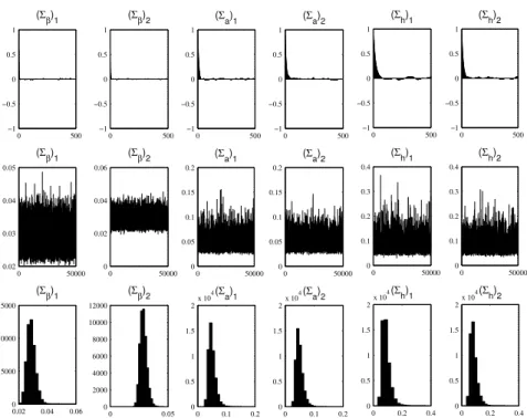
In order to compute the posterior estimates, we draw M = 50,000 samples after the initial 5,000 samples were discarded in the burn-in period. Figure (3) presents the sample autocorrelation function, the sample paths and the posterior densities for selected parameters. In general, the sampling method efficiently produces uncorrelated samples, since the sample paths look stable
and the sample autocorrelations drop stably.
Table (2) provides the estimates for posterior means, standard deviations, the 95% credible intervals, the convergence diagnostics (CD)15, and the
inef-ficiency factors16of Geweke (1992). According to the CD statistics obtained,
one should observe that the null hypothesis of the convergence to the poste-rior distribution is not rejected for the parameters at the 10% significance le-vel. Moreover, the sampling for the parameters and state variables is efficient
since the inefficiency factors are rather low.
Tabela 2: Estimation Results of Selected Parameters in the TVP-VAR model
Parameter Mean Std. Dev. 95% Interval CD Inefficiency
(Σβ)1 0.0203 0.0021 [0.0167;0.0248] 0.327 3.91
(Σβ)2 0.0203 0.0021 [0.0167;0.0248] 0.245 3.55
(Σ
a)1 0.0501 0.0127 [0.0322;0.0807] 0.478 21.06
(Σ
a)2 0.0481 0.0114 [0.0316;0.0757] 0.764 19.48
(Σh)1 0.0612 0.0189 [0.0360;0.1075] 0.933 32.72
(Σh)2 0.0597 0.0176 [0.0357;0.1044] 0.607 31.51
Notes: The term “Std. Dev.” refers to the standard deviation.
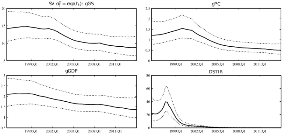
Figure (4) plots the posterior estimates of stochastic volatility of the struc-tural shock,σt2= exp(hit), on four variables, based on the posterior mean, and the one-standard-deviation intervals. Regarding the time-varying volatility of the government spending growth rate, the period from 1996–2002 displays a
data available was applied(source: IBGE).
14Regarding the short-term interest rate (STIR), solely the usual difference operator was
ap-plied to the series. One should note that the results for the short-term interest rate in its level
are divergent among themselves. Since the tests depicted stationarity for its first difference, the
model was therefore estimated using the STIR as a I(1) process. However, as a robustness check, the model was also estimated with STIR being a I(0) process. The results were not considered
qualitatively different from the ones presented in this paper. These results are available upon
request from the author.
15Following Geweke (1992), the CD statistics can be obtained by CD = ( ¯x
0 −
¯
x1)/ q
ˆ
σ02/n0+ ˆσ12/n1, where n0 and n1 are respectively the first and the last ndraws, ¯xj =
(1/nj)P mj+nj−1
i=mj x
(i),x(i)is thei-th draw, andqσˆ2
j/nj is the standard error of ¯xj, forj= 0,1. If
the sequence of the MCMC sampling is stationary, then it converges in distribution to a standard
normal. Based on Nakajima et al. (2009), we setm0= 1,n0= 5,000,m1= 25,001 andn1= 25,000,
while the ˆσj2is obtained using a Parzen window with bandwidthBm= 500.
16The inefficiency factor is defined as 1 + 2PBm
s=1ρs, withρsbeing the sample autocorrelation
at lags. This factor measures how well the MCMC chain mixes. Besides, when the ineffi
ci-ency factor is equal tok, we need to drawktimes as many MCMC samples as uncorrelated
sam-ples. For instance, the inefficiency factor for (Σβ)1is 4.18, which implies that we obtain about
0 500 −1
0 1
(Σ β)1
0 50.000 0.01 0.02 0.03 0.04 (Σ β)1
0 0.02 0.04 0
5000 10000 15000
(Σβ)1
0 500
−1 0 1
(Σ β)2
0 50.000 0.01 0.02 0.03 0.04 (Σ β)2
0 0.02 0.04 0
5000 10000 15000
(Σβ)2
0 500
−1 0 1
(Σa)1
0 50.000
0 0.1 0.2
(Σa)
1
0 0.1 0.2 0
10.000 20.000
(Σa)1
0 500
−1 0 1
(Σa)2
0 50.000
0 0.1 0.2
(Σa)
2
0 0.1 0.2 0
10.000 20.000
(Σa)2
0 500
−1 0 1
(Σh)1
0 50.000
0 0.2 0.4
(Σh)
1
0 0.2 0.4 0
10.000 20.000 30.000
(Σh)1
0 500
−1 0 1
(Σh)2
0 50.000
0 0.2 0.4
(Σh)
2
0 0.2 0.4 0
10.000 20.000
(Σh)2
Notes: Sample autocorrelations (top), sample paths (middle) and posterior densities (bottom).
Figura 3: Estimation Results of Selected Parameters in the TVP-VAR model
higher volatility level as compared to the period from 2002 onwards. The dampening behavior, and later stability, is in agreement with the establish-ment of the Brazilian Fiscal Responsibility Law (FRL) in 2000, which impo-sed limits to government budget in order to achieve the solvency of the public debt.
1999:Q1 2002:Q1 2005:Q1 2008:Q1 2011:Q1
5 10 15 20 SV✁ 2
t= exp(ht): gGS
1999:Q1 2002:Q1 2005:Q1 2008:Q1 2011:Q1
0.5 1 1.5 2 2.5 3 gGDP
1999:Q1 2002:Q1 2005:Q1 2008:Q1 2011:Q1
0 20 40 60
80 DSTIR
1999:Q1 2002:Q1 2005:Q1 2008:Q1 2011:Q1
0 0.5 1 1.5 2 2.5 gPC
Notes: The terms gGS, gPC and gGDP refer to government spending, private consumption and GDP growth rates, respectively. DSTIR is the short-term interest rate in its first
difference. Only median responses are reported. Posterior mean (solid line) and 95%
credible intervals (dotted line).
Figura 4: Posterior Estimates for Stochastic Volatility
credit expansions which increase the liquidity of Brazilian households and, therefore, have smoothed their intertemporal consumption (Steter 2013).
In mid-1999, less than six months after moving to a floating exchange rate system, Brazil adopted an inflation-targeting framework for monetary policy. The short-term interest rate thus became the Brazilian Central Bank’s main instrument to manage inflation. Moreover, since the Brazilian government es-tablished a sustained fiscal austerity, the Monetary Policy Committee (Copom) decided in favor of a downward bias, as public debt is indexed to the short-term interest rate. Therefore, the estimated time-varying volatility for its first difference drops sharply until 2000, reaching values close to zero towards the
rest of the sample. This result further corroborates the empirical evidences of a smoothing behavior for the short-term interest rates during the inflation-targeting regime.
But how have the simultaneous relations among the variables changed over time? Based on the recursive identification from the lower triangular matrixAt, one can obtain the posterior estimates of the free elements inA−t1, denoted ˜ait. In other words, these free elements depict the size of the simulta-neous effect of other variables to one unit of the structural shock17, presented
in Figure (5).
1999:Q1 2002:Q1 2005:Q1 2008:Q1 2011:Q1 0
0.5 1
˜
a1t(At1: gGS✂gGDP)
1999:Q1 2002:Q1 2005:Q1 2008:Q1 2011:Q1 −1
−0.5 0 0.5
˜
a2t(gGS✂DSTIR)
1999:Q1 2002:Q1 2005:Q1 2008:Q1 2011:Q1 −0.5
0 0.5
˜
a3t(gGDP✂DSTIR)
1999:Q1 2002:Q1 2005:Q1 2008:Q1 2011:Q1 −0.5
0 0.5 1
˜ a4t(gGS✂gPC)
1999:Q1 2002:Q1 2005:Q1 2008:Q1 2011:Q1 0
0.5 1
˜ a5t(gGDP✂gPC)
1999:Q1 2002:Q1 2005:Q1 2008:Q1 2011:Q1 −0.5
0 0.5
˜
a6t(DSTIR✂gPC)
Notes: The terms gGS, gPC and gGDP refer to government spending, private consumption and GDP growth rates, respectively. DSTIR is the short-term interest rate in its first
difference. Only median responses are reported. Posterior mean (solid line) and 95%
credible intervals (dotted line).
Figura 5: Posterior Estimates for Simultaneous Relations
The simultaneous relations of the short-term interest rate in its first dif-ferences to the government spending growth rate shock ( ˜a2t: gGS →DSTIR) are negative and vary over time, going from near -0.3 in 1996 to almost zero in 2014. Similarly, the simultaneous relations of the private consumption growth rate to the short-term interest rate in its first differences ( ˜a6t: DSTIR
→gPC) are negative throughout the sample, but more constant than the latter. Furthermore, the estimated results suggest that these relationships are insig-nificantly different from zero since the probability bands include the zero line.
17With exception of the short-term interest rate in its first difference, the variables presented
Both simultaneous relations of the GDP growth rates to the government spending growth rate shock ( ˜a1t: gGS →gGDP) and the private consumption growth rates to the GDP growth rate shock ( ˜a5t: gGDP →gPC) stay positive and rather constant over the sample period. Also, with respect to the simul-taneous relations of the private consumption growth rates to the government spending growth rate shock ( ˜a4t: gGS →gPC), these are positive and rather volatile between 1996 and 2003, following a downward trend. From Lula’s election onwards, the relations remains almost constant.
Even though the simultaneous relation of the short-term interest rate in its first differences to the GDP growth rate shock ( ˜a3t:gGDP→DSTIR) is
insigni-ficantly different from zero until 2007, changes in the GDP growth seems to
positively affect the interest rate thereafter, with the positive relation spiking
in mid-2010. This might imply that the interest rate dynamics has become more responsive to the business cycle fluctuations after the recent global fi-nancial crisis.
3.1 (In)Effectiveness of Government Spending Shocks
Since the time-varying VAR framework is able to compute state-dependent impulse responses at each individual quarter, potential changes on the macro-economic dynamics can be evaluated over the sample period. As proposed by Nakajima (2011), these impulse responses are calculated after fixing an initial shock size equal to the time-series average of stochastic volatility over the sample period, using the simultaneous relations at each point in time, in order to achieve comparability over time.
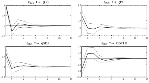
Figure (6) reports the estimated time-varying impulse responses for the variables to a positive government spending growth rate shock18. The results show that the recovery of the government spending growth rate to its initial level was more volatile at the beginning of the sample, even though the overall response is rather similar throughout the entire period.
Regarding the short-term interest rate, the effects of spending shocks are
negative at first, turning positive after the second quarter until reaching the initial level on the fifth quarter onwards. Kirchner et al. (2010), addressing the effects of fiscal stimulus with an estimated TVP-VAR for the Euro Area,
found similar results. One possible explanation for this behavior is the Bra-zilian government’s commitment to the fiscal debt solvency, mainly since the FRL in 2000. Furthermore, the effects of spending shocks on the interest rate
have lost persistence over time.
But how effective is discretionary fiscal policy in stimulating economic
ac-tivity? We can immediately observe that the spending shocks increase private consumption and the GDP growth rates, which is in line with other Brazilian studies (e.g. Mendonça et al. (2009), Carvalho & Valli (2010) and Peres (2012)). As discussed in Reis et al. (1998), and later corroborated in Gomes (2004), ne-arly 80% of Brazilian households are non-Ricardian and thus consume their income period by period. Consequently, the positive estimated effects of
Bra-zil’s fiscal stimulus arises from the fact that therule-of-thumbconsumption, to an extent sufficient, compensates the potential negative effects from Ricardian
agents. Also, the initial impulse responses are larger at the beginning of the sample, whereas the shock persistence seems to have decreased after Lula’s
0
5
10 1999:Q1
2005:Q1 2011:Q1 −0.5
0 0.5 1 1.5
Horizon εgGS ↑→ gP C
Time (t)
Impulse
0
5
10 1999:Q1
2005:Q1 2011:Q1 0
2 4
Horizon εgGS ↑→ gGS
Time (t)
Impulse 0
5
10 1999:Q1
2005:Q1 2011:Q1 −0.5
0 0.5 1 1.5
Horizon εgGS ↑→ gGDP
Time (t)
Impulse
0
5
10 1999:Q1
2005:Q1 2011:Q1 −1
0 1
Horizon
εgGS ↑→ DST I R
Time (t)
Impulse
Notes: The terms gGS, gPC and gGDP refer to government spending, private consumption and GDP growth rates, respectively. DSTIR is the short-term interest rate in its first
difference. Only median responses are reported.
Figura 6: Time-Varying Impulse Responses
election at the end of 2002. As for the GDP growth rate results, the initial effectiveness of the fiscal stimulus decreased throughout the sample. On the
other hand, the results further suggest that the effects on GDP have gained
persistence from 2005 onwards.
Even though the time-varying responses maintained a similar pattern from mid-1996 until late-2014, the results suggest that the government spending shocks could be indeed considered effective in promoting economic activity,
but are only sustained on the short-run since positive effects are on average
visible only until the horizon of four quarters. Silva & Cândido Júnior (2009) argue that this limited efficacy in stimulating macroeconomic aggregates
th-rough fiscal policy is a common feature among Latin America countries. Still, the time-varying techniques indicate some increasing persistence of the latter shocks effectiveness. In general, the results are in line with the recent
Bra-zilian literature on fiscal policy (Mendonça et al. 2009, Peres 2012, Soave & Sakurai 2012).
3.2 Time-Invariant Comparison: A BVAR Approach
2005, Primiceri 2005, Koop et al. 2009).
While the previous empirical approach highlighted that the time-varying interplay of government spending and private consumption can be conside-red relevant for Brazilian data, the sample spams for a relatively short period (1996:Q1–2014:Q2). Given that the Brazilian economy has undergone few structural changes throughout these years, such as the abandonment of the crawling peg exchange rate regime on January 15, 1999 and the IT framework implementation in June of the same year, we now turn the attention to the impulse responses of a time-invariant Bayesian VAR (BVAR) for government spending shocks as a comparison to the TVP-VAR model.
Define a reduced-form VAR model as:
Yt=XtA+εt εt∼N(0,Σ) (11)
whereA= (a0, A1, . . . , Ap)
′
andXt = (X1, . . . , XT)
′
. Through some matrix alge-bra, Equation (11) can be rewritten in the form of:
yt=Ztα+εt (12)
withZt= (IM⊗Xt) andα=vec(A).
The likelihood function can be obtained by the sampling density,p(y|α,Σ).
We impose a diffuse (or Jeffreys’) prior forαandΣ, so that:
p(α,Σ)∝ |Σ|−(M+1)/2 (13)
Viewed as a function of the parameters, this problem can be split into two parts: (i) a normal distribution forαgivenΣ; and (ii) an inverse-Wishart
distribution forΣ. That is:
α|Σ, y∼N( ˆα,Σ) (14)
and
Σ|y∼IW(bS, T−K) (15)
whereAb= (X′X)−1(X′Y) is the OLS estimate of A, ˆα=vec(Ab) is a vector which
stacks all the VAR coefficients (and the intercepts),bS = (Y−XAb)′(Y−XAb) is the sum of squared errors of the VAR, andbΣ=bS/(T−K) is the OLS estimate
ofΣ.
According to the results in Figure (7), the recovery of the government spen-ding to its initial level requires around five quarters. Despite some volatile behavior between 1994–2005 on Figure (6), the time-invariant dynamics is rather similar. To a lesser extent, the effects of spending shocks on private
consumption also resembles the time-varying ones.
As to the effectiveness of discretionary fiscal policy on stimulating GDP
growth, we observe positive response of output to an increase in the govern-ment spending. Even though corroborating the results previously obtained, the time-varying impulse responses revealed a growing shock persistence from the end of 2002 onwards. Hence, by applying a time-invariant BVAR model, one would underestimate the government capability to promote economic ac-tivity in the recent years.
2 4 6 8 10 12
−0.5
0 0.5 1
εgGS↑→ gGS
2 4 6 8 10 12
−0.5
0 0.5 1
εgGS↑→ gGDP
2 4 6 8 10 12
−0.6 −0.4 −0.2
0 0.2 0.4
εgGS↑→ DST I R
2 4 6 8 10 12
−0.5
0 0.5 1 1.5
εgGS↑→ gP C
Notes: The terms gGS, gPC and gGDP refer to government spending, private consumption and GDP growth rates, respectively. DSTIR is the short-term interest rate in its first
difference. Posterior mean (solid line) and 95% credible intervals (dotted line).
Figura 7: Time-Invariant Impulse Responses of Government Spending Shocks
thereafter until reaching its initial level after 18 months. However, according to Figure (6), the intensity with which STIR decreases is not constant over time, and neither is the shock persistence. The shortcomings of the time-invariant analysis are threefold: (i) it underestimates the positive response after the second quarter in the first half of the sample period; (ii) it does not capture the gradual decrease of STIR response after 2000s, and (iii) it displays a smaller shock persistence for the recent years.
Overall, despite the time-invariant impulse responses closely following the pattern of their time-varying counterparts, BVAR usually underestimates the magnitude of these responses as well as the shock persistence, especially in the last years. That is, the TVP-VAR should thus be considered an appro-priate method to overcome the issues concerning parameter uncertainty. Still, regardless of time features, the estimated impulse responses seem to be sus-tained only on the short-run.
3.3 Prior Sensitivity Analysis: Model Robustness
In order to address any potential divergence on the results due to prior speci-fication, we specify alternative priors for the TVP-VAR model. Therefore, we re-estimate it based on two different sets of diffuse and uninformative priors.
The first prior set has an alternative value for the mean of parameters (Σβ)−2
i , (Σa)−2
i and (Σh)−i2, while the second set of priors focuses on the variance of these terms19:
19One should notice that by imposing a more flexible prior for the covariance matrix ofA,
the Bayesian estimation process was not able to achieve the inverse matrix ofAdue to
singula-rity. Therefore, in order to avoid implausible behaviors of the time-varying contemporaneous
relationships parameters, (Σa)−2
i is specified as in Section 2.1. See Koop & Korobilis (2010) for
(I) (Σ
β)−i2∼G(40,0.01I), (Σa)−i2∼G(10,0.01), (Σh)−i2∼G(10,0.01)
(II) (Σβ)−2
i ∼G(25,0.02I), (Σa)−i2∼G(4,0.01), (Σh)i−2∼G(4,0.02)
The posterior estimates were obtained by drawing M = 50,000 samples
after the initial 5,000 samples were discarded in the burn-in period. The com-plete results can be found in Appendix Apêndice A. In general, both alterna-tive specifications led to similar results in comparison to the chosen priors in Section 2.1. As Figure A.2 and Figure A.3 show that the sample paths look stable and the sample autocorrelations drop stably, the sampling method ef-ficiently generates uncorrelated samples. These results are corroborated by Table A.1 and Table A.2 since the CD statistics imply that the null hypothesis of convergence to the posterior distribution is not rejected at the 10% signifi-cance level for both alternative prior sets. Moreover, the Inefficiency factors
are rather low on both specifications.
The obtained results robustly confirm the downward trend of the stochas-tic volatility in the sample period, thus reaffirming the stable macroeconomic
profile in the recent years. Posterior estimates for simultaneous relations also displayed a robust behavior in comparison to the baseline TVP-VAR model. Ergo, the robustness tests evolve consistently with the previous results.
4 Conclusions
In this paper we presented empirical evidences of the relationship between government spending and private consumption in Brazil. We estimated a vec-tor auvec-toregression model with drifting coefficients and stochastic volatility for
Brazil over the period 1996:Q1–2014:Q2.
The findings suggest that the effectiveness of spending shocks in
stimula-ting economic activity has increased since 2007, depicstimula-ting positive Keynesian multipliers. The estimated time-varying impulse responses of GDP growth rate also shows higher persistence in the recent years. However, these positive effects are only sustained on the short-run. Regarding private consumption,
the results further suggest acrowding-ineffect, despite the decrease of the
ini-tial positive response over the sample. In general, the latter results are in line with the recent literature on fiscal policy (Mendonça et al. 2009, Peres 2012, Soave & Sakurai 2012). Moreover, we document that the estimated effects of
government spending growth rate shocks on private consumption growth rate seem rather time-invariant during this period.
By comparing time-invariant impulse responses of a Bayesian VAR (BVAR) with their time-varying counterpart, we were further able to provide empi-rical evidences that parameter uncertainty might be overcome with a TVP-VAR specification. Additionally, robustness analysis confirmed the downward trend of the stochastic volatility in the period, thus reaffirming that Brazil has
steadily improved its macroeconomic stability in the recent years.
Referências Bibliográficas
Barro, R. J. (1974), ‘Are governments bonds net wealth?’,Journal of Political
Economy82(6), 1095–1117.
Barro, R. J. & King, R. G. (1984), ‘Time-separable preferences and intertemporal-substitution models of business cycles’, Quarterly Journal of
Economics99(4), 817–839.
Baxter, M. & King, R. G. (1993), ‘Fiscal policy in general equilibrium’,
Ame-rican Economic Review83(3), 315–334.
Blanchard, O. J. (1985), ‘Debt, deficits and finite horizons’,Journal of Political
Economy93(2), 223–247.
Blanchard, O. J. & Perotti, R. (2002), ‘An empirical characterization of the dynamic effects of changes in government spending and taxes on output’,
Quarterly Journal of Economics117(4), 1329–1368.
Caldara, D. & Kamps, C. (2008), ‘What are the effects of fiscal policy shocks?
a VAR-based comparative analysis’,Working Paper Series877. European Cen-tral Bank.
Canova, F. (1993), ‘Modeling and forecasting exchange rates using a Bayesian time varying coefficient model’, Journal of Economic Dynamics and Control
17, 233–262.
Carvalho, F. A. & Valli, M. (2010), An estimated DSGE model with
govern-ment investgovern-ment and primary surplus rule: The Brazilian case, in‘XXXII
Encontro Brasileiro de Econometria’, Sociedade Brasileira de Econometria.
Coenen, G. & Straub, R. (2005), ‘Does government spending crowd in private
consumption? Theory and empirical evidence for the Euro area’, Working
Paper Series513. European Central Bank.
Cogan, J. F., Cwik, T., Taylor, J. B. & Wieland, V. (2010), ‘New Keynesian versus old Keynesian government spending multipliers’,Journal of Economic
Dynamics and Control34, 281–295.
Cogley, T. & Sargent, T. (2005), ‘Drifts and volatilities: Monetary policies and
outcomes in the post WWII U.S.’, Review of Economic Dynamics 8(2), 262–
302.
Cwik, T. & Wieland, V. (2011), ‘Keynesian government spending multipliers and spillovers in the Euro area’,Economic Policy67, 493–549.
Dickey, D. & Fuller, W. (1981), ‘Likelihood ratio statistics for autoregressive time series with a unit root’,Econometrica49, 1057–1072.
Fatás, A. & Mihov, I. (2001), ‘The effects of fiscal policy on consumption and
employment: Theory and evidence’,CEPR Discussion Papers2760.
Fisher, J. D. M. & Peters, R. (2009), ‘Using stock returns to identify govern-ment spending shocks’, Working Paper Series 03. Federal Reserve Bank of Chicago.
Forni, L., Monteforte, L. & Sessa, L. (2009), ‘The general equilibrium ef-fects of fiscal policy: Estimates for the Euro area’,Journal of Public Economics
Freitas, M. C. P. (2009), ‘Os efeitos da crise global no Brasil: aversão ao risco e preferência pela liquidez no mercado de crédito’,Estudos Avançados
23(66), 125–145.
Furceri, D. & Mourougane, A. (2010), ‘The effects of fiscal policy on output:
A DSGE analysis’,OECD Economics Department Working Papers770. OECD
Publishing.
Galí, J., López-Salido, J. D. & Vallés, J. (2007), ‘Understanding the effects
of government spending on consumption’,Journal of the European Economic
Association5(1), 227–270.
Geweke, J. (1992), Evaluating the accuracy of sampling-based approaches to the calculation of posterior moments,inJ. M. Bernardo, J. O. Berger, A. P. Dawid & A. F. M. Smith, eds, ‘Bayesian Statistics’, Vol. 4, New York: Oxford University Press, pp. 169–188.
Gomes, F. A. R. (2004), ‘Consumo no Brasil: teoria da renda permanente, formação de hábito e restrição à liquidez’, Revista Brasileira de Economia
58(3), 381–402.
Hamilton, J. (1989), ‘A new approach to the economic analysis of nonstatio-nary time series and the business cycle’,Econometrica57(2), 357–384.
Hamilton, J. (2010), Macroeconomics and ARCH,inT. Bollerslev, J. R. Rus-sell & M. Watson, eds, ‘Festschrift in Honor of Robert F. Engle’, Oxford Uni-versity Press, pp. 79–96.
Hansen, N. J. H. & Sulla, O. (2013), ‘Credit growth in Latin America: Finan-cial development or credit boom?’,IMF Working Papers13/106. International Monetary Fund.
Ilzetzki, E., Mendoza, E. G. & Végh, C. (2013), ‘How big (small?) are fiscal multipliers?’,Journal of Monetary Economics60(2), 239–254.
Kirchner, M., Cimadomo, J. & Hauptmeier, S. (2010), ‘Transmision of govern-ment spending shocks in the Euro area: Time variation and driving forces’,
Working Paper Series1219. European Central Bank.
Koop, G. & Korobilis, D. (2010), ‘Bayesian multivariate time series methods
for empirical macroeconomics’, Foundations and Trends in Econometrics
2, 267–358.
Koop, G., Leon-Gonzalez, R. & Strachan, R. W. (2009), ‘On the evolution of the monetary policy transmission mechanism’,Journal of Economic Dynamics
and Control33, 997–1017.
Kwiatkowski, D., Phillips, P., Schmidt, P. & Shin, J. (1992), ‘Testing the null hypothesis of stationarity against the alternative of a unit root’, Journal of
Econometrics54, 159–178.
Linnemann, L. (2006), ‘The effect of government spending on private
con-sumption: a puzzle?’,Journal of Money, Credit and Banking38(7), 1715–1736.
Lucas, R. E. (1976), ‘Econometric policy evaluation: a critique’,
Carnegie-Rochester Conference Series on Public Policy1, 19–46.
Mankiw, G. N. & Summers, L. H. (1984), ‘Do long-term interest rates overre-act to short-term interest rates?’,NBER Working Paper1345. National Bureau of Economic Research.
Mankiw, N. G. (2000), ‘The savers-spenders theory of fiscal policy’,American
Economic Review90(2), 120–125.
Mendonça, M. J. C., Medrano, L. A. T. & Sachsida, A. (2009), ‘Avaliando os efeitos da política fiscal no Brasil: resultados de um procedimento de identifi-cação agnóstica’,Texto para Discussão1377. Instituto de Pesquisa Econômica Aplicada.
Mountford, A. & Uhlig, H. (2009), ‘What are the effects of fiscal policy
shocks?’,Journal of Applied Econometrics24(6), 960–992.
Nakajima, J. (2011), ‘Time-varying parameter VAR model with stochastic vo-latility: an overview of methodology and empirical applications’,Discussion
PaperE–9. Institute for Monetary and Economic Studies (IMES).
Nakajima, J., Kasuya, M. & Watanabe, T. (2009), ‘Bayesian analysis of time-varying parameter vector autoregressive model for Japanese economy and monetary policy’,Discussion PaperE–13. Institute for Monetary and Econo-mic Studies (IMES).
Pereira, M. C. & Lopes, A. S. (2010), ‘Time-varying fiscal policy in the U.S.’,
Working Papers21. Banco de Portugal, Economics and Research Department.
Peres, M. A. F. (2012), Dinâmica dos Choques Fiscais no Brasil, Doutorado, Universidade de Brasília - UnB.
Perotti, R. (2002), ‘Estimating the effects of fiscal policy in OECD countries’,
Working Paper Series168. European Central Bank.
Perotti, R. (2007), ‘In search of the transmission mechanism of fiscal policy’,
NBER Working Paper Series13143. National Bureau of Economic Research.
Primiceri, G. (2005), ‘Time-varying structural vector autoregressions and monetary policy’,Review of Econometric Studies72, 821–852.
Ramey, V. A. (2008), ‘Identifying government spending shocks: it’s all in the timing’,NBER Working Paper15464. National Bureau of Economic Research.
Ratto, M., Röger, W. & in’t Veld, J. (2009), ‘Quest III: An estimated open-economy DSGE model of the Euro area with fiscal and monetary policy’,
Economic Modelling26(1), 222–233.
Ravn, M., Schmitt-Grohé, S. & Uribe, M. (2006), ‘Deep habits’, Review of
Economic Studies73(1), 195–218.
Silva, A. M. A. & Cândido Júnior, J. O. (2009), ‘Impactos macroeconômicos dos gastos públicos na américa latina’,Texto para Discussão1434. Instituto de Pesquisa Econômica Aplicada.
Silva, F. S. & Portugal, M. S. (2010), Impacto de choques fiscais na economia
brasileira: uma abordagem DSGE,in‘XXXII Encontro Brasileiro de
Econo-metria’, Sociedade Brasileira de Econometria.
Sims, C. A. (1980), ‘Macroeconomics and reality’,Econometrica48(1), 1–48.
Smets, F. & Wouters, R. (2003), ‘An estimated stochastic dynamic general equilibrium model of the Euro area’,Journal of the European Economic
Associ-ation1(5), 1123–1175.
Soave, G. P. & Sakurai, S. N. (2012), Uma análise da relação de longo prazo entre o consumo privado e os gastos do governo: Evidências de países
de-senvolvidos e em desenvolvimento,in‘XL Encontro Nacional de Economia
(ANPEC)’, ssociação Nacional dos Centros de Pós-Graduação em Economia.
Steter, E. R. (2013), Expansão do Crédito e Suavização do consumo na econo-mia brasileira, Mestrado, Fundação Getúlio Vargas - FGV.
Tagkalakis, A. (2008), ‘The effects of fiscal policy on consumption in
Apêndice A Supplementary Figures and Tables
0
5
10 1999:Q1
2005:Q1 2011:Q1 2.6
2.8 3 3.2 3.4
Horizon
εgGS ↑→ gGS
Time (t)
Impulse
0
5
10 1999:Q1
2005:Q1 2011:Q1
−3 −2 −1
0 1
Horizon εgGS ↑→ DST I R
Time (t)
Impulse
0
5
10 1999:Q1
2005:Q1 2011:Q1 0
1 2
Horizon
εgGS ↑→ gP C
Time (t)
Impulse
0
5
10 1999:Q1
2005:Q1 2011:Q1 0.5
1 1.5 2
Horizon
εgGS ↑→ gGDP
Time (t)
Impulse
Notes: The terms gGS, gPC and gGDP refer to government spending, private consumption and GDP growth rates, respectively. DSTIR is the short-term interest rate in its first
difference. Only median responses are reported.
Figura A.1: Accumulated Time-Varying Impulse Responses
Tabela A.1: Estimation Results of Selected Parameters in the TVP-VAR mo-del – First Prior Set – Robustness Check
Parameter Mean Std. Dev. 95% Interval CD Inefficiency
(Σ
β)1 0.0159 0.0013 [0.0137;0.0187] 0.407 2.78
(Σβ)2 0.0159 0.0013 [0.0137;0.0187] 0.422 2.78
(Σa)1 0.0319 0.0051 [0.0238;0.0436] 0.829 9.24
(Σa)2 0.0319 0.0051 [0.0238;0.0435] 0.496 7.38
(Σh)1 0.0345 0.0063 [0.0249;0.0488] 0.675 14.74
(Σh)2 0.0339 0.0060 [0.0247;0.0479] 0.932 12.89
Tabela A.2: Estimation Results of Selected Parameters in the TVP-VAR mo-del – Second Prior Set – Robustness Check
Parameter Mean Std. Dev. 95% Interval CD Inefficiency
(Σβ)1 0.0287 0.0029 [0.0237;0.0349] 0.459 3.45
(Σβ)2 0.0287 0.0030 [0.0236;0.0352] 0.106 4.60
(Σ
a)1 0.0498 0.0124 [0.0322;0.0800] 0.716 17.38
(Σ
a)2 0.0494 0.0121 [0.0321;0.0791] 0.581 14.57
(Σ
h)1 0.0895 0.0297 [0.0516;0.1627] 0.603 36.33
(Σh)2 0.0832 0.0243 [0.0497;0.1428] 0.114 33.30
Notes: The term “Std. Dev.” refers to the standard deviation.
0 500 −1 −0.5 0 0.5 1
(Σβ)1
0 5
x 104 0.01
0.015 0.02 0.025
(Σβ)1
0.01 0.02 0.03 0
5000 10000 15000
(Σβ)1
0 500 −1 −0.5 0 0.5 1 (Σ
β)2
0 5
x 104 0.01
0.015 0.02 0.025
(Σβ)2
0.01 0.02 0.03 0
5000 10000 15000
(Σβ)2
0 500 −1 −0.5 0 0.5 1
(Σa)1
0 5
x 104 0 0.02 0.04 0.06 0.08 0.1 (Σ
a)1
0 0.05 0.1 0
0.5 1 1.5 2
x 104(Σa)1
0 500 −1 −0.5 0 0.5 1
(Σa)2
0 5
x 104 0 0.02 0.04 0.06 0.08 0.1
(Σa)2
0 0.05 0.1 0
5000 10000 15000
(Σ
a)2
0 500 −1 −0.5 0 0.5 1 (Σ
h)1
0 5
x 104 0 0.02 0.04 0.06 0.08 0.1
(Σh)1
0 0.05 0.1 0
0.5 1 1.5
2x 10
4(Σ
h)1
0 500 −1 −0.5 0 0.5 1 (Σ
h)2
0 5
x 104 0 0.02 0.04 0.06 0.08 0.1
(Σh)2
0 0.05 0.1 0
5000 10000 15000
(Σ
h)2
Notes: Sample autocorrelations (top), sample paths (middle) and posterior densities (bottom).
0 500 −1 −0.5 0 0.5 1
(Σβ)1
0 50000
0.02 0.03 0.04 0.05
(Σβ)1
0.02 0.04 0.06 0
5000 10000 15000
(Σ
β)1
0 500 −1 −0.5 0 0.5 1
(Σβ)2
0 50000
0 0.02 0.04 0.06
(Σβ)2
0 0.05 0 2000 4000 6000 8000 10000 12000 (Σ
β)2
0 500 −1 −0.5 0 0.5 1
(Σa)1
0 50000 0 0.05 0.1 0.15 0.2 (Σ
a)1
0 0.1 0.2 0
0.5 1 1.5 2
x 104(Σa)1
0 500 −1 −0.5 0 0.5 1
(Σa)2
0 50000 0 0.05 0.1 0.15 0.2 (Σ
a)2
0 0.1 0.2 0
0.5 1 1.5 2
x 104(Σa)2
0 500 −1 −0.5 0 0.5 1
(Σh)1
0 50000 0 0.1 0.2 0.3 0.4
(Σh)1
0 0.2 0.4 0
0.5 1 1.5
2x 10
4(Σ
h)1
0 500 −1 −0.5 0 0.5 1
(Σh)2
0 50000 0 0.1 0.2 0.3 0.4
(Σh)2
0 0.2 0.4 0
0.5 1 1.5
2x 10
4(Σ
h)2
Notes: Sample autocorrelations (top), sample paths (middle) and posterior densities (bottom).
Figura A.3: Estimation Results of Selected Parameters in the TVP-VAR model – Second Prior Set – Robustness Check
1999:Q1 2003:Q1 2007:Q1 2011:Q1
10 15 20 25
SVσ2
t= exp(ht): gGS
1999:Q1 2003:Q1 2007:Q1 2011:Q1
2 2.5 3 3.5 4 4.5 gGDP
1999:Q1 2003:Q1 2007:Q1 2011:Q1
0 10 20 30
40 DSTIR
1999:Q1 2003:Q1 2007:Q1 2011:Q1
0.5 1 1.5 2 2.5 gPC
Notes: The terms gGS, gPC and gGDP refer to government spending, private consumption and GDP growth rates, respectively. DSTIR is the short-term interest rate in its first
difference. Only median responses are reported. Posterior mean (solid line) and 95%
credible intervals (dotted line).
1999:Q1 2003:Q1 2007:Q1 2011:Q1 5
10 15 20 25 30
SVσ2
t= exp(ht): gGS
1999:Q1 2003:Q1 2007:Q1 2011:Q1
1 2 3 4 5
6 gGDP
1999:Q1 2003:Q1 2007:Q1 2011:Q1
0 10 20 30 40
50 DSTIR
1999:Q1 2003:Q1 2007:Q1 2011:Q1
0 1 2 3
4 gPC
Notes: The terms gGS, gPC and gGDP refer to government spending, private consumption and GDP growth rates, respectively. DSTIR is the short-term interest rate in its first
difference. Only median responses are reported. Posterior mean (solid line) and 95%
credible intervals (dotted line).
Figura A.5: Posterior Estimates for Stochastic Volatility – Second Prior Set – Robustness Check
1999:Q1 2003:Q1 2007:Q1 2011:Q1
0 0.2 0.4 0.6 0.8 1
˜
a1t(A−t1: gGS→gGDP)
1999:Q1 2003:Q1 2007:Q1 2011:Q1
−1
−0.5
0 0.5
˜
a2t(gGS→DSTIR)
1999:Q1 2003:Q1 2007:Q1 2011:Q1
−0.5 0 0.5
˜
a3t(gGDP→DSTIR)
1999:Q1 2003:Q1 2007:Q1 2011:Q1
0 0.2 0.4 0.6 0.8 1
˜
a4t(gGS→gPC)
1999:Q1 2003:Q1 2007:Q1 2011:Q1
0.4 0.5 0.6 0.7 0.8 0.9 1
˜
a5t(gGDP→gPC)
1999:Q1 2003:Q1 2007:Q1 2011:Q1
−0.5
0 0.5
˜
a6t(DSTIR→gPC)
Notes: The terms gGS, gPC and gGDP refer to government spending, private consumption and GDP growth rates, respectively. DSTIR is the short-term interest rate in its first
difference. Only median responses are reported. Posterior mean (solid line) and 95%
credible intervals (dotted line).
1999:Q1 2003:Q1 2007:Q1 2011:Q1 0
0.2 0.4 0.6 0.8 1
˜
a1t(A−t1: gGS→gGDP)
1999:Q1 2003:Q1 2007:Q1 2011:Q1
−1 −0.5 0 0.5
˜
a2t(gGS→DSTIR)
1999:Q1 2003:Q1 2007:Q1 2011:Q1
−0.5
0 0.5
˜
a3t(gGDP→DSTIR)
1999:Q1 2003:Q1 2007:Q1 2011:Q1
0 0.2 0.4 0.6 0.8 1
˜
a4t(gGS→gPC)
1999:Q1 2003:Q1 2007:Q1 2011:Q1
0.4 0.5 0.6 0.7 0.8 0.9 1
˜
a5t(gGDP→gPC)
1999:Q1 2003:Q1 2007:Q1 2011:Q1
−1
−0.5
0 0.5
˜
a6t(DSTIR→gPC)
Notes: The terms gGS, gPC and gGDP refer to government spending, private consumption and GDP growth rates, respectively. DSTIR is the short-term interest rate in its first
difference. Only median responses are reported. Posterior mean (solid line) and 95%
credible intervals (dotted line).