Time Poverty in Brazil:
Measurement and Analysis of
its Determinants
Lilian Lopes Ribeiro
Doutoranda - Curso de Pós-Graduação em Economia (CAEN/UFC)
Endereço para contato: Av. da Universidade, 2700 - 2º andar CEP: 60120-181 E-mail: [email protected]
Emerson Marinho Professor (CAEN/UFC)
Endereço para contato: Av. da Universidade, 2700 - 2º andar CEP: 60120-181 E-mail: [email protected]
Recebido em 26 de outubro de 2010. Aceito em 15 de fevereiro de 2012.
Abstract
This article analyzes well-being on an individual level, through the allocation of work hours done by adults and children and thus it measures time poverty in Brazil. In order to achieve such measurement, poverty indicators such as Foster, Greer and Thorbecke (FGT) were adapted into a time poverty mode. Additionally, an analysis of its determinants was also conducted. Among other findings, the fact that women (either children and adult ones) are the time-poorest individuals in urban or rural areas. Another unfortunate finding is that the high rate of time poverty among children, numerically 16,1% is not far from the adult rate which is of 19,7%. The overall composite time poor individual profile is of an African-Brazilian adult woman of little education, not necessarily income poor and residing in an urban area of the northeast region, living in a household of few people, she is the mother of children who are younger than 14 years old.
Keywords
time poverty, well-being, time allocation
Resumo
Palavras-Chave
pobreza de tempo, bem-estar, alocação de tempo
1. Introduction
In recent years, economic literature on poverty has been devoted on studying the importance of time use in economic analysis. Many studies about the job market analyze, the increase of individual work hours due to time restriction as did Newman (2002). Other aspects were analyzed by Blackden and Bhaun (1999), Gelb (2001) and Apps (2004), who bring up a wide discussion about uses and restrictions of time in the economic development of countries. There is a consen-sus among researchers that individual well-being is not determined only by income or consumption rates, but also by other conditioners. Sen (1999) and Vickery (1977) believe that individual income are unsatisfying limited indicators for measurements of individual well-being and life quality. These authors believe that despite income is still vital to people´s lives, it should not be considered a most important instrument for well-being measurements. Studies conduc-ted by Vickery (1977), Douthitt (1994), Damián (2003), Ilahi and Nadeem (2000,2001), Bardasi and Wodon (2006) show that time as a resource is as important as income. Different from income and consumption and their the-more-the-merrier approach, time is a scarce resource and more time allocated for work, productive or not, means less leisure and less rest, and therefore higher time poverty. One of the advantages of the time poverty approach is the possibi-lity of conducting studies about individual well-being, which is not possible through measurements of income and consumption.
Various agencies, national and international ones, have been pointing out that exhausting work hours lead to many health problems such as nervous breakdowns, depression, repetitive strain injuries, besides jeopardizing family cohesion due to lack of time devoted to family.
So, by acknowledging that poverty measurements should not only consider income but also other kinds of deprivations, this article con-tributes to the literature about the subject by conducting a study on poverty in the Brazilian economy using individual time deprivation as a parameter. After all, two individuals or two families of same income may have different time resources and that will affect well-being in two distinct ways.
Using 2009 PNADdata, this article about time poverty in Brazil was originally inspired by the concept of time allocation as a well-being indicator. An individual is considered time-poor if the total amount of his or her weekly work hours, be it full time, part-time or hou-sehold work, exceeds the poverty line.
The time poverty measurement is calculated by adapting the FGT (Foster, Greer and Thorbecke (1984) income poverty measurements, that is, adapting the FGT to the specific time poverty case. The in-dicators are: the proportion of poor individuals who are time poor, the time poverty that measures its intensity and the square time poverty hiatus which measures its severity. They are calculated con-sidering the gender of adults and children per urban and rural areas and the Brazilian regions. Through the marginal effects of a logit econometric model, the impact of various determiners that explain time poverty in Brazil are also analyzed.
Among many results, whatever the time poverty indicators, women in Brazil (either children or adults) are the time-poorest individuals in both urban and rural areas. Another disturbing result is the high proportion of time poverty for children, about 16,1%, not very far from the adult population rate 19,7%.
a falling tendency. People with children younger than 14 years old show higher probability of being time poor, whilst the bigger number of family members the less likely an individual is to be time-poor.
The article, besides this introduction, is distributed along five more sections. The second section presents a bibliographical revision about time poverty. On the third section, time poverty is formally defi-ned and a poverty line is constructed. The fourth section shows the results of the time poverty indicators. On the fifth section, a logit econometric model is specified and its results are analyzed. The sixth and last section is devoted to the article´s main conclusions.
2. Time Poverty: A Brief Account
The concept of time poverty was first used by Vickery (1977) in order to identify families with time unavailability which kept them from attaining the U.S. well-being level, due to long working hours, so often taken out of sheer necessity and not by choice. The study about time poverty focuses its analysis on time spent doing house activities as much as on time spent on productive activities Bardasi & Wodon (2006).
The main goal of the Vickery (1977) article was to define a bidimen-sional measurement of well-being, not only under a monetary point-of-view but also defining the amount of time needed to achieve a minimum consumption level, once for this to take place, both inco-me and tiinco-me are required. This way, families would be considered poor if they possessed a certain combination of time and money.
This subject of study has grown in importance also for the International Labour Organization (ILO) that developed international standards based on the idea that long working hours mean a health hazard to both workers and their families. According to Bardasi and Wodon (2009), these standards have been widely applied in order to guarantee workers´ health.
Burchardt (2008), in his survey conducted in various countries con-siders time as a vital component of well-being. Damián (2003) wrote this about the importance of using the time factor for the measure-ment of well-being:
“Let´s think of two hypothetical households which income is equal to the poverty line of $ 1,000.00 per capita and these households would not be considered poor if the income criterion were applied. The first household is formed by Juan, his wife and his 3 year-old son. Juan earns $ 3,000.00 and his wife takes care of the child and the housework. The second household is formed by Ana and her 6 month-old son. Ana is a housemaid who earns $ 2,000.00. She doesn´t have anyone else to take care of her son and she can´t afford a day-care service. Thus, she must lock him in a room so she can go to work. Although similar from an income perspective, these two households show a huge difference in terms of time availability and quality of living”.
Neither Juan or Ana are considered time-poor if the criterion used is the sole income figure. However, Ana suffers from time deprivation for she does not have whom to leave her son with. Such deprivation keeps her from enjoying the same levels of well-being and quality of living that Juan enjoys, once taking care of her baby makes Ana a time-poor individual.
Recently, in face of increasing unemployment rates in developed countries, one of the reasons to study time poverty is to show the evolution of male and female roles in housework. On the studies by Kes and Swaminathan (2006), conducted for the Sub-Saharan and the studies by Bardasi and Wodon (2009), commissioned by and about Guinea-Bissau, there is an underestimation of fema-le participation in formal work, due to time devoted to non-re-munerated activities such as housework, taking care of pre-school age children or taking care of sick individuals. All these factors lead to reduction of available time that could otherwise be devo-ted to productive activities and leading to income poverty as well.
Literature shows that Brazil has registered a speedy growth of the inclusion rate of women in the job market since the eighties. Médici, (1989) apud Aquino et al. (1995) point out that between 1976 and 1985, there was an increase in the number of economically active women at the geometric yearly rate of 5,6%, against only 2,9% of similar male increase.
This trend has a positive effect, once articles by Kes and Swaminathan (2006), and by Bardasi and Wodon (2009) women who carry out remunerated work tend to invest a higher percentage of their expenses on human capital which in the long term tends to reduce time poverty and income poverty.
A methodological slip pointed out by Bardasi and Wodon (2009) is that on many studies about time poverty is the lack of data on time adults devote to taking care of children and handicapped individuals. This, according to the authors, leads to underestimation of results. Besides, there is no clear border between what should be considered work and what should be regarded as leisure. Should taking care of one´s community be considered work or leisure? That is a question of subjective nature.
3. Deinition and Construction of the Poverty Line
available by the Brazilian Institute of Geography and Statistics (IBGE). The definitions of all variables are described as follows.
The variables that were used to construct the poverty line: number of weekly hours spent on primary work, secondary work and all other work plus time spent commuting plus number of weekly hours spent on housework.1
The time poverty determinants of the econometric model specified on Section 5 of this article, are represented by the variables: monthly income of all work done for people older or as old as 10 years old; number of people residing in the household (including people resi-ding there as tenants, house employees and their relatives); years of education; age of occupants at the date of reference. Additionally, dummies variables were constructed for the variables of gender, race, parents of children younger than 14 years old; individuals who live with children younger than 5 years old who go to day-care; individu-als who live with people older than 75 years old, on urban or rural areas.
The PNAD data were chosen due to their completeness and com-prehensive scope about populational characteristics such as educa-tion, work, income and especially the number of hours devoted to primary work, secondary work and housework. Data so important for the construction of the poverty line and also invaluable for the calculation of poverty line indicators. Besides, it allows an individu-al level survey or even an interregionindividu-al survey, which would not be possible by using other existing data bases.
An individual is considered time-poor if his/her total of weekly work hours, be it at primary work, secondary work or other work (remu-nerated by the formal sector or the informal one) or even housework and the commuting time, named
t
i is bigger than a certainpre-determined poverty line2 t.
1 Housework is defined as doing these activities at one´s home a) partial or total cleaning of
the residence; b) cooking or preparing foods, ironing, laundry work, dish washing by using appliances or not, in order to execute these tasks for oneself or any other residing person; c) guiding or supervising of house workers during their performance of duties; d) looking after one´s children or other residing children; e) cleaning the yard or the home´s surrounding area (IBGE, 2010).
2
Then, one can calculate the following FGT- type indicators: pro-portion of time-poor individuals (P0), time poverty hiatus (
P
1) and square time poverty hiatus(P2).The measure P0 is defined as
P
0=
N
p/
N
, where Np is the numberof time-poor individuals, that is, the number of people in which
t
t
i>
and N is the size of the population older than 10 years old. In this case, P0 measures the exact proportion of time-poor individuals.The indicator P1 is defined as
∑
=
−
=
Npi i
t
t
t
N
P
11
(
)
1
. This last one
measures the average deficit of time in relation to the poverty line t.
It is the measurement of intensity of time poverty. In a similar way,
the square poverty hiatus is defined as
∑
=
−
=
p N i it
t
t
N
P
1 22
(
)
1
.
As the average time deficit in relation to the poverty line is potentia-poverty line is potentia-lized to the square, higher values are attributed to those who show higher overtime work hours. That is, as higher values are given to the time-poor individuals among them, this indicator measures the severity of time poverty.
3.1 The Construction of the Time Poverty Line
On their study for Guinea-Bissau, Bardasi and Wodon (2006) defi-ned the time poverty line as the median of the total amount of hours worked by an individual, plus times 1,5 the value of such median and thus establishing an inferior limit and twice as big as the value of the median for the superior limit. Kalenkoski et al. (2008) and Burchardt (2008) in their articles also used the median of the total hours worked plus 50%, 60% and 70% added to such figure.
hours from the sample happened to be mostly symmetrical, we cho-se to ucho-se the average of this variable instead of the median of it. The construction of the inferior and superior limits of the time poverty line is done somewhere ahead.
For calculating the total amount of allocated leisure hours by indi-vidual, the number was subtracted from the total amount of avai-lable self-care hours, which involve basic care such as eating, sho-wer-taking and getting dressed, plus the total weekly hours of sleep needed for an individual to keep his/her physical and mental health. Weekly work hours were also deducted.
This way, naming as
H
t the total amount of available weekly hours for an adult person (over 14 years old),H
s the total of weekly hours devoted to sleeping,H
p the total amount of hours spent on perso-nal care andH
h the average weekly hours spent on the job market (be it formal or informal work, and also including commuting times), the total amount of leisure hoursla
H
of an adult is calculated asla t s p h
H
H
H
H
H
.For children between 10 and 14 years old, it is necessary to de-duct from
H
t the weekly study hoursH
e. Therefore, we calllc
H
the total amount of children´s leisure hours, we come tolc t s p h e
H
H
H
H
H
H
. Calculating such figures foradults, t
H
=168, once the total amount of available hours in a weekis 158 for any person. According to the American Academy of Sleep Medicine (2007) apud Burchardt (2008), the universal number of hours of sleep needed by an individual is from 7 to 8 hours a day. If we adopt the 8-hour standard, then
H
s=56.Time spent on personal care was estimated as 14 weekly hours consi-dering 2 hours a day are enough for activities such as eating, shower-taking and getting dressed. On such terms,
H
p=14. This was alsothe standard used by Burchardt (2008).
The average hours spent in a week on the job market be it formal or informal were estimated as 53 hours according to the figures on Table 1. Therefore,
H
h=53.Then, when
la t s p h
H
H
H
H
H
is applied, it is found thatthe total number of leisure hours (
la
For children between 10 and 14, values for
H
t,H
s eH
premain unaltered, that is,H
t=168,H
s=56 andH
p =14. According to IES (2011), the standard of hours of sleep for children between 10 and 14 years old are 7 or 8 hours, the same standard of an adult. On this study, the 8 hour figure was adopted.The average hours weekly spent on the job market be it formal or informal were estimated as 25 hours, according to the figure on Table 2. Thus,
H
h= 25. Finally, the total amount of weekly hours spent on studying was estimated as 20 hours, considering that a child spends on average 4 hours a day on such activity. That is,e
H
=20. Therefore, considering thatlc t s p h e
H
H
H
H
H
H
,the total amount of leisure hours in a week ( lc
H
) is equal to 53 or asthe formula goes, lc
H
= 53.This way, the superior poverty line limit is defined as the average number of weekly work hours plus half of the total amount of we-ekly leisure hours. Its inferior limit is equal to the average number of weekly work hours plus14of the total amount of leisure hours.
Therefore, in a weekly scale, the superior and inferior poverty lines for adults are equal to 75 and 64 hours respectively. For children, these limits are equal to 51 and 37.
Although a subjective discussion might ensue regarding the ascer-tainment of the poverty line, it is necessary to state that the goal of this article is to identify individuals who belong to the upper area of the work hours distribution. That is, those who work in excess, be it at housework or remunerated work and by doing so, compromise their well-being level.
All the time poverty measurements were calculated taking into ac-count the gender of adults and children and whether individuals lived in a rural or urban area. This study categorized as children, individuals between the ages of 10 and 14, and as adults, individuals ranging from 15 to 75 years old.3
3 Previous time poverty calculations by age group showed that 22,9% of individuals between
4. Evidences about Brazil
Table 1 shows the average numbers of work hours from the sample of individuals used for the construction of the time poverty line in Brazil. The sample is comprised of 156.263 observations. The figures of this sample clearly show big differences between the numbers of average work hours by men and by women. The total amount of work hours by women (57,3 hours) is higher than the total amount of work hours by men (49,7 hours).
Table 1 - Average Number of Weekly Work Hours by Activity and Gender of Children & Adults in Brazil
Boys Girls All Male Female All
1 - Primary Work 18,4 18,3 18,4 43,6 36,0 40,4
2 - Secondary Work 0,0 0,0 0,0 0,98 0,92 0,95
3 - Other work 0,0 0,0 0,0 0,05 0,05 0,05
4 - Job Market (1+2+3) 18,5 18,4 18,5 44,6 37,0 41,4
5 - Housework 4,1 11,3 6,4 4,9 20,2 11,4
6 - Total (4+5) 22,7 29,6 25,0 49,7 57,3 53,0
Source: constructed by the authors based on PNAD (2009) data.
These same results are verifiable for children. In Brazil, girls work more than boys (29,6 hours against 22,7 hours, respectively).
Please notice that men show an average number of remunerated work hours that is higher than the women´s number. Since childhood, wo-men are overloaded with housework and work almost 4 times more than men. The same results were also verified on articles by Kes & Swaminathan (2006) and Bardasi & Wodon (2006, 2009) on the Sub-Saharan Africa.
4.1 Analysis of the Time Poverty Indicators
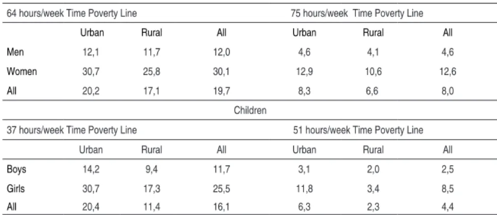
These results remain true for the rural and urban areas. For adults, the proportions of time-poor men and women in urban areas are 12,1% and 30,7%, respectively. In rural areas, these percentages are equal to 11,7% and 25,8%. Women are, therefore, more time-poor than men in either urban or rural areas.
Certainly, women are more time-poor because they allocate more time for house chores. Dedecca (2004), when analyzing time uses in Brazil and in the world, found out that in 2001, 42% of European men declared they did housework while 90% of women said the same. In Brazil, according to the same author, women also have hi-gher scores when it comes to allocating time for housework.
Table 2 - Proportion of Time-Poor Individuals by Area and Gender in Brazil
Adults
64 hours/week Time Poverty Line 75 hours/week Time Poverty Line
Urban Rural All Urban Rural All
Men 12,1 11,7 12,0 4,6 4,1 4,6
Women 30,7 25,8 30,1 12,9 10,6 12,6
All 20,2 17,1 19,7 8,3 6,6 8,0
Children
37 hours/week Time Poverty Line 51 hours/week Time Poverty Line
Urban Rural All Urban Rural All
Boys 14,2 9,4 11,7 3,1 2,0 2,5
Girls 30,7 17,3 25,5 11,8 3,4 8,5
All 20,4 11,4 16,1 6,3 2,3 4,4
Source: constructed by the authors based on PNAD data.
So, the
Burchardt (2008) assumption also holds true for Brazil. According to her, individuals who are the most time-poor spend more time on non-remunerated activities such as house chores and they also spend less time on the job market, which contributes for poverty increase in the future.The proportion of time-poor children in rural areas, 11,4%, is less than the proportion in urban areas, that is of 20,4%. From these percentages, 17,3% correspond to girls and 9,4% to boys, both in rural areas. In urban areas, the numbers are respectively 30,7% and 14,2%. These results lead to the conclusion that, once again, in both urban and rural areas, female children are more time-poor than male children.4
Based on the evidence shown, one can surmise that such reality for children and especially for girls, might result in longer education delays or even drop-outs, which compromises their well-being in adult life. Another important finding by Schwartzman et al. (2004) is that the education levels of Brazilian mothers have a noticeable effect in reducing child labour in all income groups and therefore, an impact on the time poverty of children.
The numbers on Tables 3 and 4 show, respectively, the results of time poverty hiatus and square time poverty hiatus by gender and area for both poverty. These two indicators measure respectively, the intensity and the severity of time poverty.
Table 3 - Time Poverty Hiatus by Area and Gender in Brazil (percentage)
64 hours/week Time Poverty Line 75 hours/week Time Poverty Line
Urban Rural All Urban Rural All
Men 1,7 1,6 1,7 0,5 0,5 0,5
Women 4,8 3,8 4,7 1,7 1,3 1,7
All 3,0 2,4 3,0 0,7 2,4 0,9
37 hours/week Time Poverty Line 51 hours/week Time Poverty Line
Urban Rural All Urban Rural All
Boys 2,8 1,5 2,1 0,5 0,3 0,4
Girls 7,8 3,1 6,0 2,3 0,3 1,5
All 4,7 2,1 3,4 0,3 0,8 0,7
Source: constructed by the authors based on PNAD (2009) data.
Using as a reference the inferior time poverty line on Table 3, we see that 3,0% of adults are intensely time-poor. There is a substantial proportion of intensely poor women (4,7%) in comparison to the percentage of men (1,7%). However, what draws the most attention are the results of the female children. 7,8% of girls in urban areas are intensely time-poor.
4
Although the numbers on Table 4 show that there is a small propor-tion of individuals in severe time poverty, once again females score a higher considerable percentage in comparison to males. Among children, 2,8% of girls living in urban areas are extremely time-poor and suffer from severe time deprivation that leaves them with not enough time for school or even leisure.
Table 4 - Square Time Poverty Hiatus by Area and Gender in Brazil (percentage)
64 hours/week Time Poverty Line 75 hours/week Time Poverty Line
Urban Rural All Urban Rural All
Men 0,4 0,3 0,4 0,1 0,0 0,0
Women 1,1 0,8 1,0 0,3 0,2 0,3
All 0,7 0,5 0,7 0,0 0,0 0,0
37 hours/week Time Poverty Line 51 hours/week Time Poverty Line
Urban Rural All Urban Rural All
Boys 0,8 0,4 0,6 0,1 0,0 0,0
Girls 2,8 0,7 1,9 0,6 0,0 0,4
All 1,4 0,5 1,0 0,3 0,0 0,2
Source: constructed by the authors based on PNAD (2009) data.
5. The Econometric Model and its Results
In order to identify and analyze time poverty conditioners, as well as their marginal effects, a logit econometric model was specified under these terms:
2
0 1 2 3 4 5 6 7
8 9 10 11 12 13
14 15 16
5 14 75
i i i i i i i i
i i i i i i
i i i i
P rend ida ida nPess esc Dmasc Durb
Dme nc Dme Dma Dneg Dout DNo
DNe Se Sul
in which the variable
]
1
ln[
i i i
p
p
P
−
=
is the defined as the logarithmof the probability reasoning in favor of the do i-numbered individual to be time-poor. The idiosyncratic error εi follows a distribution of
logistical probability.5
5 If
Individual personal characteristics are represented by these expla-natory variables: rend is the work income, ida is age in years, ida2 is square age in years, esc are the education years, nPess is the total number of family members. Besides these determiners, other con-trols were added to the model, such as gender, race, family make up, urban/rural areas residence and Brazilian regions. All these con-trols are respectively represented on Model (1) by these dummy variables:
Dmasc
• : gets 1 (one) if the individual is male and 0 (zero) if female;
Durb
• : gets 1 (one) if the individual resides in an urban area and 0 (zero) if in rural area;
Dme5nc
• : gets 1 (one) if the individual lives with children younger than 5 years old who do not go to day care and 0 (zero) if otherwise;
Dme14
• : gets 1 (one) if an individual lives with children youn-ger than 14 years old and 0 (zero) if otherwise;
Dma75
• : gets 1 (one) if an individual lives with people older than 75 years old and 0 (zero) if otherwise;
Dneg
• : gets 1 (one) if an individual is of black ethnicity and 0 (zero) if otherwise;
Dout
• : gets 1 (one) if an individual is neither of white or black ethnicity and 0 (zero) if otherwise;
DNo
• : gets1 (one) if an individual resides on the North region and 0 (zero) if otherwise;
DNe
• : gets 1 (one) if an individual resides on the Northeast region and 0 (zero) if otherwise;
DSul
• : gets 1 (one) if an individual resides on the South region and 0 (zero) if otherwise and,
DSe
• : gets 1 (one) if an individual resides on the Southeast region and 0 (zero) if otherwise.
( ) e / (1 e ), .
Its density function is symmetrical around zero with
0(zero) average and the density function is around zero with average and variance 2 / 3
5.1 Results of the Econometric Model
Table 5 shows the marginal effect figures of the logit regression Model (1) considering, respectively, inferior and superior limits of time poverty.
The estimated marginal effects seen on this table, although not using the inferior or superior limits of poverty as markers, are not very dis-crepant. The analysis will be done considering only the inferior limit as an exception if any significant result differences come about.
Table 5 - Marginal Effects for the Probability of an Individual to be Time-Poor in Brazil, Using the Inferior and Superior Limits of the Time Poverty Line
Variables dy/dx dy/dx* standard
deviation
standard
deviation* Z z* Value-p Value-p* rendi 3.42e-06 1.34e-06 0.000 0.000 3.62 2.32 0.020 0.000
ida i 0.017 0.007 0.0004 0.0002 49.20 28.02 0.000 0.000
ida2 i -0.0001 -0.00008 0.0001 0.000 -46.42 -25.82 0.000 0.000
nPess i -0.009 -0.002 0.001 0.000 -16.66 -6.84 0.000 0.000
Esci -0.005 -0.002 0.000 0.000 -16.95 -12.31 0.000 0.000
Dmasci -0.167 -0.071 0.002 0.001 -83.94 -52.20 0.000 0.000
Durb i 0.029 0.016 0.003 0.001 11.50 11.39 0.000 0.000
Dme5nci -0.005 -0.014 0.004 0.006 -1.18 -2.21 0.027 0.238
Dme14i -0.023 -0.019 0.014 0.009 -1.66 -2.09 0.037 0.097
Dma75i 0.007 0.001 0.006 0.003 1.09 0.30 0.762 0.277
DNeg i 0.010 0.004 0.004 0.002 2.79 1.87 0.062 0.005
Dout i 0.008 0.004 0.002 0.001 4.13 3.63 0.000 0.000
DNO i -0.015 -0.006 0.004 0.002 -4.24 -2.62 0.009 0.000
DNE i 0.023 0.018 0.003 0.002 7.40 8.31 0.000 0.000
DSE i 0.018 0.010 0.003 0.002 5.87 4.75 0.000 0.000
DSUL i 0.016 0.006 0.003 0.002 4.57 2.56 0.011 0.000
The p-values of the income, education, age and square age variables show that they are all statistically significant. The positive marginal effect that was estimated about income reveals that the probability of an individual to be time-poor increases although such effect is considerably small. After all, in general terms, higher income levels might be associated to intense job market activity which leads to little time left for leisure.
The evidence of time poverty increasing as an individual is younger and diminishing as he or she gets older seems to be true. The signs of marginal effects of variable the ida and ida2 variables are respecti-vely, positive and negative besides being both statistically significant. In other words, the time poverty trajectory throughout one´s life turn out to get the shape of an inverted letter u. That is, its marginal effects are positive for younger individuals and negative for senior ones, revealing that time poverty tends to diminish after a certain age. These same results were verified by Bardasi and Wodon (2006). In the Brazilian economy, every increase of one year of age equals to an approximately 2% probability increase of one being time-poor.
The increase of the number of people living in the same household contributes to a smaller propensity of an individual to be time-poor. The estimated marginal effect of this variable shows that one addi-tional person in the household will cause a reduction of 0,9% to the probability of an individual to be time-poor. Probably as house chores are usually distributed among the members of the household, this lessens their chances of being time-poor. Such result coincides with the one obtained by Lawson (2007) for the Sub-Saharan Africa, the Bardasi & Wodon (2006, 2009) results for Guinea-Bissau and the Kalenkoski et al. (2008) results for the United States.
Regarding the marginal effects of individual education, results show that the increase in the average number of school years tend to re-duce one´s chances of being time-poor. Possibly, people of higher education have more skills and are therefore more productive. That means their housework and job market activities are accomplished in less time thus leaving more available time for leisure.
individu-al to be time-poor. On the contrary to these results, Lawson (2007) identified for the Sub-Saharan Africa that those of higher education are more likely to be time-poor. Probably, the specific circumstan-ces of the region make people devote more time not only to the job market but to their housework as well.
The fact of a person being male reduces by 16,7% his chances of being time-poor. This negative correlation was also spotted by Burchardt (2008) for the United Kingdom. On the other hand, these results contradict evidence obtained by Bardasi and Wodon (2006) for Guinea-Bissau, a country where men are more likely to be time-poor. Among determinants of time poverty, the male person characteristic is the one that has contributed the most for lessening the chances of someone to fall into time poverty. In Brazil, although female participation in the job market has increased significantly, male participation is still predominant. Generally, women besides working in the job market, also spent a great deal of their time doing housework. This makes them more likely to be time-poor.
The propensity one has of being time-poor, increases by 2,9 % for those who reside in urban areas in comparison to those living in rural ones. Somehow, these results seem to confirm the numbers on Table 2, where 20,4% of people who reside in urban areas are time-poor against only 17,1% of time-poor people living in rural areas.
A surprising result was that of children below five years old who do not attend day-care. Such fact actually lessens the probability of a person to be time-poor. The usual expectation is that children demand a lot of time and attention and therefore bring their pa-rents into time poverty. But for papa-rents who can buy help in the housework job market, the probability of time poverty may actually lessen under such circumstances.
The dummy variable Dme14i, included in the model in order to test
Regarding individuals who live with senior citizens older than seven-ty-five years old, results are not statistically significant whatever the time poverty limit. Despite the expected increase in time poverty probability for the case, in Brazil it is very usual for grandparents to take care of their grandchildren and by doing this, grandparents compensate for the time they the elderly require from their relati-ves. Probably the net result of such interactions will affect nobody´s individual time poverty.
When it comes to the race characteristic, results show that Afro-Brazilian individuals are more sensitive to time deprivation than white individuals. The fact of being Afro-Brazilian increases in 1% the chances one has of being time-poor. The same goes for other ra-ces like (indigenous, multiracial or Asian) who also get a 1% increase. Burchardt (2008) also states that ethnic minorities are more time-poor than other ethnicities.
For last, using the Midwest region to establish a comparison, we see that Brazil´s North region inhabitants are the ones who show the smallest propensity to be time-poor. For those residing in the remaining Brazilian regions, there is on average an increase of 2% in the probability of being time-poor. Regarding such result, in more developed regions where the job market is more competitive, de-manding more work hours from individuals, and the cost of help is usually higher, the probability of a person to be time-poor might increase due to these factors.
6. Final Thoughts
As for children, the time poverty proportion calculated using its inferior limit is 16,1%, not so distant from the adults´ proportion. Out of the children´s proportion 11,7% are boys and 25,5% are girls. Female children are also more time-poor than male ones in both urban and rural areas. Though in different proportions, this scenario does not get very different when the superior time poverty limit is applied. These results are somewhat concerning, for the overtime these children spend on other activities is detrimental to their edu-cation and might affect their future.
Among the time poverty determinants, work income tends to in-crease the probability of an individual to be time-poor while more people living in the same household and more years of education tend to lessen such probability.
Another evidence found is that time poverty probability increases when someone is young and begins to decrease after certain adult age. In other words, the time poverty trajectory throughout time has the shape of an inverted letter u.
The male gender characteristic reduces a person´s probability of being time-poor in 16,7%. Among all time poverty determinants, this is the one that contributes the most for the decrease of one´s probability of being time-poor. In Brazil, women besides spending time on work hours also dispose of a big portion of their time on housework and thus becoming more likely to be time-poor.
People who have children younger than five years old who do not attend day-care show a smaller increase of their probability of being time-poor. This result defies common sense as the usual expecta-tion portrays these children requiring more time and attenexpecta-tion from parents who in their turn become more time-poor. However, there is still the possibility of buying the help from a third party in the housework job market which would actually make the time poverty probability drop.
Regarding the race characteristic, the results show that African-Brazilians are more sensitive to time deprivation in comparison to individuals of white race. It happens likewise to people of other ethnicities such as indigenous, half-breeds and Asians. This result matches with the international evidence which says ethnic minorities are more time-poor than predominant races.
For last, using the Midwest region in a comparison to other regions, results show that the inhabitants of the North region are the ones with the smallest propensity to be time-poor. After the evidence produced by the survey, it is now possible to present a composite profile of a typical time-poor individual in Brazil. An adult black woman of little education, not necessarily income poor, residing in an urban area of the Northeast region. She lives in a household with few other people and is the mother of children younger than four-teen years old.
References
Aquino, E. M. L; Meneses, G. M. S; Marinho, L. F. B. Mulher, Saúde e Trabalho no Brasil: Desaios para um Novo Agir. Rio de Janeiro. Caderno de Saúde Pública.v. 11, nº02, p.281-290. 1995. Apps, P. Gender, Time Use, and Models of the Household. Washington, D. C: World Bank, 2004. (Policy
Research Working Paper Series: 3233).
Bardasi, E.; Wodon, Q. Measuring Time Poverty and Analyzing Its Determinants: Concepts and Appli-cation to Guinea: Gender, Time Use, and Poverty in Sub-Saharan Africa. Washington, DC: Word Bank, 2006. (World Bank Working Paper, Nº. 73, p. 75-95).
Bardasi, E.; Wodon, Q. Working long hours and having no choice: time poverty in Guinea. Washington, DC: Word Bank, 2009. (Policy Research Working Paper Series 4961).
Blackden, C. M.; Bhanu C. Gender, Growth, and Poverty Reduction. Special Program of Assistance for Africa 1998 Status Report on Poverty. Washington, DC: Word Bank, 1999. (Paper Nº. 428).
Burchardt, T. Time an income poverty. CASE Report 57, London. 2008. (Centre for Analysis of Social Exclusion, London School of Economics).
Damián, A. La pobreza de tiempo. Uma revisión metodológica, Estudios Demográicos y urbanos. v. 18, nº. 52, p.127-162. 2003.
Dedecca, C. Tempo, trabalho e gênero. Reconiguração das relações de gênero no trabalho. CUT - Central Única dos Trabalhadores. São Paulo, 2004. http://library.fes.de/pdf-iles. Accessed in 07 de august de 2011.
Douthitt, R. A. Time to do the Chores? Factoring Home-Production Needs into Measures of Poverty. Vol. 21 nº 1, 7-22. Journal of family and economic issues, 1994.
Foster, J.; Greer, J.; Thorbecke, E. A Class of Decomposable Poverty Indices, Econometrica. v.52, n.3, p.761-766.1984.
Harvey, A. S.; Taylor, M. 1996. An LSMS Time-use Module Department of Economics, St. Mary’s University, mimeograph.
Ilahi, N. Gender and the Allocation of Adult Time: Evidence from the Peru LSMS Panel Data, Policy Research Working Paper Series No. 2744, World Bank, 2001.
Ilahi, N. The Intra-household Allocation of Time and Tasks: What Have We Learnt from the Empirical Literature? Policy Research Report on Gender and Development, Working Paper Series Nº. 13, Washington, DC: World Bank Development Research Group, 2000.
Instituto Brasileiro de Geograia e Estatística (IBGE). Pesquisa Nacional por Amostra em Domicílio– PNAD 2009. Rio de Janeiro: IBGE, 2009.
Instituto de Epilepsia e Sono (IES). O sono de uma criança. Goiânia, 2011.
Kalenkoski, C. M.; Hamrick, K; Andrews, M. Time Poverty Thresholds. Ohio University, 2008. (Eco-nomic Research Service Nº. 58-4000-6-0120).
Kes, A.; Swaminathan, H. Gender and time poverty in sub-Saharan Africa. Washington DC: Word Bank, 2006. (Paper Nº. 73. World Bank).
Lawson, D. A. Gendered Analysis of Time Poverty: The Importance of Infrastructure. Department of Economics. Manor Road, Oxford, Reino Unido, 2007. Available in: <http://www.economics. ox.ac.uk/ accessed in 03 de November de 2010.
Long, J.; Freze, J. Regression models for categorical dependent variables using Stata. College Station: Stata. Press, 2001.
Newman, C. Gender, Time Use, and Change:The Impact of the Cut Flower Industry in Ecuador. World Bank Economic Review. v. 16, p. 375-95. 2002.
Schwartzman, S. O trabalho infantil no Brasil. Instituto de Estudos do Trabalho e Sociedade, UFRJ. Rio de Janeiro, 2004. Available in: http://www.schwartzman.org.br. Accessed in 07 de august de 2011.
Sen, A. Development as Freedom. Oxford: Oxford University Press, 1999.