J. Transp. Lit. vol.8 número2

Key words: airline cost function, translog model, econometric models.

Palavras-Chave: função de custo de companhia aérea, modelo translog, modelos econométricos.

Recommended Citation Resumo

Este trabalho continua e estende vários temas de estudos anteriores de funções de custo de companhias aéreas comerciais. Uma função de custo industrial bem especificada revela características sobre os participantes de mercado, tais como economias de escala e as elasticidades de custo relativas a características operacionais. Usando uma especificação translog e sua forma restrita de primeira ordem, este artigo atualiza as estimativas anteriores da literatura, retrabalha o projeto do experimento, e proporciona uma nova análise para descrever o espectro de escolhas pelas quais as empresas aéreas vem enfrentando nos últimos anos. O modelo translog neste artigo possibilita que a participação dos custos de combustível nos custos totais seja interagida com outras variáveis, permitindo um esclarecimento dos fatores que podem agravar a sensibilidade dos custos aos preços do combustível - um avanço nesta área específica de interpretação. O resultado mostra que as participações de custos do combustível tendem a ser maiores com equipamentos mais antigos, com frotas menores, e tendem a ser crescentes com o tamanho e densidade de assentos das aeronaves. O modelo restrito de primeira ordem indica que aeronaves mais antigas possuem operações mais custosa, mesmo levando em consideração o estilo operacional da empresa. Isto pode implicar que as companhias aéreas com menos acesso ao capital sofrem uma desvantagem de custos, particularmente durante um pico de preços de combustível - o que também constitui uma contribuição do artigo. Finalmente, o modelo de primeira ordem não rejeita a hipótese de retornos constantes de escala para a expansão da frota, ou retornos crescentes com o tamanho das aeronaves, que são os resultados esperados.

Meland, W. J. (2014) Measurement of a cost function for US airlines: restricted and unrestricted translog models. Journal of Transport Literature, vol. 8, n. 2, pp. 38-72.

William J. Meland*

Abstract

This paper continues and expands several themes from previous studies of commercial airline cost functions. A well specified industrial cost function reveals characteristics about the market players, such as economies of scale and the cost elasticities with respect to operational styles. Using a translog specification, and its restricted first-order form, this paper updates previous parameter estimates, reworks the experimental design, and gives new analysis to describe the spectrum of choices facing airline firms in recent years. The translog model in this paper allows the energy cost share to interact with other variables and illuminate what factors may exacerbate cost sensitivity to energy prices, an advance in this specific area of interpretation. The result shows that fuel cost shares tend to be higher with older equipment, smaller fleet sizes, and to be increasing in aircraft size and seating density. The restricted first-order model indicates that older aircraft designs are more costly to operate, even accounting for operational style. This may imply that airlines with poorer access to capital suffer a cost disadvantage, particularly during a fuel spike – also a new contribution of the paper. Finally, the first-order model does not reject constant returns to scale (CRS) for fleet expansion, or increasing returns to scale (IRS) in aircraft size, which are the expected results.

* Email: wmeland@gmail.com.

Research Directory

Submitted 7 Jan 2013; received in revised form 28 Mar 2013; accepted 16 Jun 2013

Measurement of a cost function for US airlines:

restricted and unrestricted translog models

[Mensuração de uma função de custo para companhias aéreas norte-americanas: modelos translog restritos e irrestritos]

University of Minnesota - United States

Introduction

This paper updates prior literature by calibrating a translog cost function of US airlines for

recent years, using an engineering-centric, fleet-based approach. All costs are modeled at the

fleet by fleet. Fortunately, data sources exist for these fleet-level costs. Other parameters are

specified to help control for operational style: average flight stage length, seats per aircraft,

fleet count, number of airports served by the fleet and airline, etc. By doing this, coefficients

in the results should effectively model cost impacts of marginal changes in fleet

characteristics – adding seats, flying longer distances, or employing older or newer

equipment. Throughout, the aim is to produce a model sufficiently disaggregated that it could

be used to model the cost of realistic operational changes, acknowledging that cost centers of

aircraft fleets can be quite independent of others within the same firm.

Historically, the cost function has been important because it can reveal to us nearly everything

about the production technology (Chambers, 1988). Here, by examining and modeling public

data, we can explain how airline firms convert inputs into outputs. We can then identify

whether the efficiency of firms appears to increase with scale. The effects of various external

shocks – elevating the price of oil, for example – can be seen in the model outputs. The

distinctions between indirect and direct costs; returns to scale; returns to scope; and fixed

effects modeling are analyzed here with respect to earlier studies.

Understanding the cost functions for airlines, or their revenue functions, can yield helpful

insights into transportation policy and/or general industrial forecasting. The most remarkable

elements of this industry, perhaps inspiring past researchers, are (1) the contestability and

commodification of players, implying efficiency; and (2) centrally collected data whose

accuracy is overseen by a regulator.

Each major US airline collects and reports many categories of quarterly cost and operational

data at the fleet level to federal regulators. This gives researchers great flexibility to test

different models. Thanks to “Form 41” data, airlines can be seen as a transparent laboratory

where firms act out strategies in a “natural” setting, governed by their own cost and revenue

Competitively, a “settling out” process has been in progress since formal US air market

deregulation in 1978. That implies that the domestic market is fairly “contestable.” If so, a

single cost function could be applied across all companies in the market, representing “state

of the art” production technology. This paper proceeds (as others have) with the assumption

that one cost model generally applies.

I first construct a cost function for recent data using methods similar to Caves, Christensen

and Tretheway (1984). In the full translog result, I find that elasticity of total cost with

respect to fuel price (equivalently, fuel’s cost share) tends to be higher with older equipment,

and also with smaller fleet sizes. Also, cost elasticity with respect to fuel price tends to be

increasing in aircraft size and seating density. Old aircraft technology, itself, appears to cause

higher costs in the restricted first-order translog model

The sections of the paper proceed as follows: 1. Literature Review; 2. Model Specification; 3.

Data and Empirical Strategy; 4. Estimation Results; Conclusion.

1. Literature Review

1.1 Rationale of the Model: Contestability

The validity of a nationwide cost model has been approached with practicality by a number of

authors. While we can measure firm operations, and fix identity labels to their data, it is

unclear whether the coefficients have a direct application in the industry. Previous authors

have implied that firms are subject to a common set of institutions, markets, technology and

the laws of physics. It is important to assert that competition does prevail, rather than some

arbitrary uncompetitive space in which costs are not necessarily relevant, such as expense

preference behavior in the regulated, as mentioned by Sickles (1986). It is most often claimed

that the markets are contestable between the players whose costs we are attempting to fit into

the common model.

A perfectly contestable market is defined as “one into which entry is completely free, from

which exit is costless, in which entrants and incumbents compete on completely symmetric

terms, and entry is not impeded by fear of retaliatory price alterations” (Baumol, Panzar,

have been mixed. I assume that the production in this study takes place in a contestable

fashion. Hence, a general set of cost elasticities (and cross-elasticities) are obtained and

reported from all firms, although the cost intercepts are unique by firm. Adoption of

contestable markets is an essential ingredient to a cost study.

1.2 Cost Model Specification Literature – Cost Model Theory

A theoretically valid cost function must exhibit certain properties (Varian, 1984). In

particular, the cost function should be:

• non-decreasing in input factor prices and output quantities;

• homogeneous of degree one in factor prices;

• concave in factor prices; and

• continuously differentiable (ideally, twice differentiable) in prices.

Also, there should be zero fixed costs, and fulfillment of Shephard’s Lemma,

such that:

dTC w

( )

dw_i =xi (1)

with wi input prices and xi input quantities.

The properties of a valid cost function are discussed in Chambers, 1984.

1.3 Cost Model Specification Literature – Engineering Based / Micro Models

Swan (2006) builds a simulation of generic airline production costs at the micro level. This

idea suggests a way to achieve the aim of the present work: to model actual airline cost data at

the micro level. The operational cost function for aircraft is described by Swan as a model

based solely on seat counts and flight distances. Swan’s model takes the form:

Other factors could be considered endogenous – and assuming CRS in fleet size, scale could

be irrelevant as well. While we lack sufficient data resolution to use this model exactly, it is

important to recognize that disaggregation has its benefits.

Aircraft ownership costs (and maintenance costs) are very real, but may reasonably be

discarded in group analysis. Swan argues that costs may equilibrate and be discarded, as “the

driver of used airplane values is the need to establish a cost position along the cost frontier...

the cost frontier itself is designated by the price of newly manufactured airplanes.” This cost

frontier could be construed as an operational indifference curve, over which profitability is

equal; thus, equipment costs could drop out.1

Morrison (1984) looks more deeply at the relationship between aircraft capital cost and the

inherent efficiency of an aircraft’s design. Uniform physical principles may underlie a

significant portion of airline cost functions. The laws of physics, with their limitations of

speed, reliability and fuel efficiency, affect aircraft operators uniformly in such a model, with

respect to the equipment they choose. Firm equipment factor demands have a point of

interface in the aircraft exchange market. As prices prevail along a cost frontier, differences

that we observe can be assigned to coefficients in a fixed-factor or fixed-effects model.

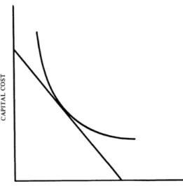
Figure 1 - Capital Operating Efficiency vs. Cost2

1

The assumption here by Swan is that a sufficiently liquid exchange market exists for used aircraft. It follows that the marginal profitability for such aircraft should be equal among firms, equalizing their lease values. 2

In Morrison’s graphic, a frontier exists between capital costs and operating costs per mile

(capital cost of aircraft versus its energy efficiency and maintenance costs). If such a frontier

is monotonic, and exchange markets are liquid, then each firm chooses aircraft at its preferred

location along that frontier, assuming all players are efficient. Like firms would choose like

equipment, at like prices. An airline might wish to buy a more expensive aircraft with lower

fuel consumption to provide a cushion against cost volatility of future fuel price spikes.

Concerns about capital shortages, meanwhile, may encourage hoarding of cash and depress

demand for new equipment temporarily.

These firm heterogeneity scenarios are each precluded by Morrison’s assumption of a single

frontier. Using the liquidity of aircraft purchasing and leasing, we are left with an operational

cost solely determined by output, exclusive of aircraft cost, which is also the method

suggested by Swan. This would perhaps rationalize new aircraft purchases at the firm level, a

key point for Swan’s employer, the Boeing Corporation, (as such purchases could be

described as cost neutral).

The feature that distinguishes the “engineering-based” approach to econometric analysis is the

analysis of a specific group of machines whose production process can be usefully understood

by a single unit of production data. This disaggregated analysis comes closer to a

“mechanical” functional form that is amenable to forecasting or static interpretation. To

report only on aggregates of machines, while it can be interpreted observationally, has limited

practicality in decision-making. Practical validity is enhanced if we have an accurate model

of the micro production choices, as they exist, because this clears away aggregation bias.

That issue is discussed directly in 1.7, and the proposed remedy in 2.3.

1.4 Cost Model Specification Literature – Panel Data of Firm Operations

Caves, Christensen and Tretheway (1984) (hereafter CCT) is the main precursor of this study.

CCT use scale and density coefficients to obtain the returns to scale (RTS) and returns to

density (RTD). Their treatment of production “density” (or, increased product per

geographical area) gives a fine substitute for scale itself within a geographic system. CCT use

the first-order coefficients of a translog for their cost model (omitting the second-order

ln[Total Cost] = β0 + β1ln[Aircraft Miles] + β2ln[points served] +

β4ln[mean flight distance] + β5[load factor] + β6[labor price] + (3)

β7[fuel price] + β8[capital-materials price] + β8[capacity] +

βi[firm identities].

Expressed symbolically, CCT did a first-order restricted translog regression:

ln

[

]

i

∑

i

∑

Firms

∑

Times

∑

Where Y is output, Wi are input prices, and the Zi are operational control variables that

describe airline characteristics, or production styles. The coefficients on ln Zican give us cost

elasticities of these characteristics.

CCT also performed both a full translog model:

Ln[TotalCost]=

α0+αYlnY+ βilnWi + φilnZi

i

∑

i

∑

2δYY(lnY)

2

+1 2

i

∑

i

∑

j

∑

j

∑

+ ρYilnYlnWi + i

∑

i

∑

j

∑

i

∑

Times

∑

Firms

∑

(5)

Here, Aircraft Miles is the output Y variable. This scale variable’s coefficient, in a regression,

tells us how unit costs would be influenced by simply repeating the activities of production

more times. This gives us an indication of whether an industry becomes more efficient as

firm size increases, i.e., whether it experiences positive “economies of scale.” In CCT, seats

and average flight distance (Stage) are held constant while Aircraft Miles, the scale variable,

grows or shrinks. Effectively, this becomes departure count,3 the logical building block of

“scale.” The partial derivative of cost with respect to Available Seat Miles (ASMs) is also

found here by using Aircraft Miles as a proxy for departures.

3

Supposing the length of haul remains the same, a doubling in aircraft miles would by definition by

CCT estimate the above coefficients both as a full translog model, and a simplified model in

which only the first-order coefficients are included. CCT report that “the coefficients for the

simplified translog form... are remarkably similar to the first-order coefficients from the basic

translog model.” This suggests that second-order coefficients were either insignificant, or

counterbalanced each other.

The interpretations of key coefficients for CCT were as follows:

• Aircraft Miles, Cost elasticity of density, identical flights, fixed network;

• Points served, the cost impact of spreading resources over an additional service point;

• Flight distance, cost of impact spreading the aircraft miles over fewer, longer flights.

• ββββ1 + ββββ2, customary elasticity of scale, allowing geographic area to expand.

1.5 Cost Model Literature – Returns to Scale, Density, Scope

Positive economies of scope suggest that, even in a contestable market, firms will produce

multiple products (or expand their networks) thanks to cross-product economies (Baumol,

1982). Without economies of scope, firms would not enter multiple cities or pursue hub

networks. Most earlier papers have observed economies of density (decreasing unit costs as

output increases in a given geographical area). They have also observed economies of scope,

at least in the sense that one firm offering two products (or two travel routes) will be more

efficient than two such firms covering that ground separately.

CCT find constant returns to scale in firm operations of the US airline industry. Economies

of scope should be assumed in our environment; as said by Baumol, “Economies of scope are

necessary for the existence of multiproduct competitive firms” (Baumol, 1982).

Gillen uses the formulation

RTS_CALE = dlnC

dln

[

]



 

 

−1

, (6)

where values above unity signify positive “returns” to scale. The reciprocal, cost elasticity of

2.1), meaning that RTS was significantly above unity, when firm dummies were included.

With firm dummies omitted, there were no significant observed economies of scale. Canadian

airline companies show increasing returns to density, when airline identities are included in

regression, but no difference from unity if they are not included (Gillen, 1985).

Caves and Tretheway, writing in the period of the initial post-deregulation shakeout following

1978, believed that low costs of entry would facilitate equilibrium slowly. Their expectation

was for any clear differences in technical efficiency among firms to abate over time, “as the

regulatory era recedes into history,” replaced by the apparently more thriving competitive

market of today. Returns to scale would favor industrial consolidation, something that has in

fact occurred dramatically since the CCT 1984 paper.

Table 1 - Prior Literature First Order Approximated4

Cost Elasticities of Scale, Density, Fuel Price

SCALE DENSITY FUEL PRICE Years

Caves (1984) .936 (se .065) .804 (se .034) .166 (se .001) 1970-1981

Gillen (1985)5 .741 (t = 2.1) .568 (t = 4.8) .04 (t = 2.3) 1964-1981

Wei (2003) 0.811 (t = 24.3)6 N/A .240 (t = 7.21) 1987-1998

Chew (2005) 1.012 (se .023)7 Not done .1106 (.0035) 1994-2001

Positive economies of scope, if found, imply that airline hubs will emerge, according to

simulation literature on the topic (Hendricks et al.,1999). Hub-spoke networks can be “a

deterrent” to the entry of smaller carriers, due to structural revenue advantages (in essence,

the revenue premium obtained by scope, as customers would prefer firms with greater

network points, affording ease of shopping). In competitive markets, the increased cost of

larger scope would apparently be justified by that revenue premium. While comparative

4

While these are from full translog models, in which interactions matter, the first order coefficients (without interactions) can signify the cost elasticities at the sample means of the data (Wei, 2003).

5

Gillen uses Canadian data. Log-linear model. The rest are U.S. only. 6

This is returns to seat count (machine scale) within single aircraft types 7

network costs are beyond the topic of their study, Hendricks says that a least-cost hub will be

located where origin and destination distances are minimized across the cumulative traffic

spectrum. This, too, explains how multiple hubs can arise in opposition to one another.

Significantly, contestability and cost advantages are not simply analyzed at the flight leg

level. Instead, airline costs represent networks that may compete from differing geographical

perches (heterogeneity, as allowed by Berry, 1992). In competition, Hendricks finds the

industry prone to monopoly due to economies of density. “Every city-pair market is

effectively served by only one carrier, the one with a length advantage [across its transfer

hub]…” Also, they note that while one hub carrier will tend to dominate, “nonhub networks

raise average costs of service but may allow the carriers to price less aggressively,” meaning

they can expect another type of revenue premium.

Table 1 shows a compendium of previous airline cost studies in which returns to scale and

density (and cost elasticity of fuel price) are obtained. While these may be expected to

change over time, and particularly as regulatory or technological characteristics varied, a

general CRS or light IRS characteristic is visible. CCT did not reject CRS in translog.

1.6 Cost Model Specification Literature – Concavity Considerations

The concavity of a cost function is one of the key conditions of its validity (Varian, 1984;

Chambers, 1988). Concavity checks of the first order log-log cost function can be done

directly by taking the second derivatives of the raw (non-logged) cost function. With the full

translog-style equation however, it is noted that a concave function is always log concave.

Therefore, by retaining logs, we can at least allow the possibility to reject (if the function is

not log concave). Improvement on that basis can be measured.

A more complete way to check concavity of a translog style function is to check the

Allen-Uzawa matrix of partial cost elasticities. Allen-partial matrix concavity implies Hessian

matrix concavity (Featherstone, 2007). For the ith cross price elasticity at each observation,

we have ηij =Sj +

b_ij

S_i , where Si is the cost share of input factor i. The equation also works

where i=j to get own-price Allen-Uzawa cost partial elasticities, from which the partials

A process has been developed to impose cost function concavity, if needed, in projects such

as CCT and the present one (Ryan and Wales, 2000). This procedure was used recently by

Chua, Kew and Yong, 2005; (hereafter, CKY). Earlier methods to impose global concavity

will negate the flexibility of the translog form. Instead, CKY and Ryan / Wales impose local

concavity. To do this, a particular data observation is designated the “normalization point.”

All its price, scale and state of nature variables are scaled to equal one; this ensures that the

cost Hessian is negative semidefinite for that observation. By selecting the normalization

point carefully, many or all of the observations’ violations of concavity can be remedied.

CKY detail several examples of cost studies whose results are questionable or reversed,

following this procedure. The CKY method of imposing local concavity maintains the

translog model’s flexibility.

Using data for 10 airlines over the period 1994 to 2001, CKY present an enhancement and

update of the earlier CCT cost estimation technique. CCT’s cost function violates concavity

at approximately half its observations. CKY were able to rehabilitate those data. They

present their new study, which includes a translog cost function. They re-estimate the CCT

cost function after imposing concavity, finding “material differences in scale economies” after

doing so. Note that the CCT and CKY papers both use aggregate corporate data. In this

paper, the concavity check recommended by CKY is used with consideration for their

normalization remedy.

Further, modeling all normalizations and choosing the best one is a feasible extension that

should prove simple and useful. Other concavity normalizations can impact flexibility of the

cost function.

1.7 Cost Model Specification Literature – Aggregation Considerations

The second recent innovation subsequent to the CCT study is a method to dis-aggregate data

when necessary. A recent translog cost estimation study provides a logical way to

disaggregate operational numbers from firms into fleets (Basso and Jara-Diaz, 2005). It is

noted that aggregate outputsy ˜ _h are implicit functions of fleet outputs Y. Looking at

operational metrics, Basso and Jara-diaz use ton-kilometeres (TK) and average length of haul

TK(Y)= y_ij⋅d_ij

ij

∑

and

ALH Y

( )

ij

∑

ij

∑

Σ

ij yij⋅dij Σijyij

 

 

  _⋅deps

type

∑

t=1

types

deps

]. (8)

Basso and Jara-diaz explain that the above applies “where dijis the distance travelled by flow

yij between origin i and destination j. Therefore, even if the true (disaggregated) product

vectors YA, YB and YD were unknown, SC [economies of scale] could still be calculated

correctly if the corresponding aggregates ˜ Y (YA) , ˜ Y (YB) and ˜ Y (YD) were known, and an

estimated cost function ˜ C ( ˜ Y ,PS) was available...”8 This is a method of rationalizing the

distribution of aggregate metrics such as average length of haul by weighting it by product, in

this case the ton-kilometer (the passenger-mile could work equivalently well, if we need a

method to distribute such costs in a passenger study).

In similar recognition of aggregation problems, another recent study uses disaggregated, fleet

level data9 to construct a translog operations cost model from Form 41 data (Wei and Hansen,

2003). This was done to study aircraft capital costs and the demand for certain aircraft types.

Their use of Form 41’s unaggregated direct operating cost data tables indicates some curiosity

about fleet-level cost analysis, something expanded in the present project. I use the same data

source tables as Wei and Hansen, together with a dis-aggregation technique similar to Basso,

as will be described in the Model section for indirect costs.

While Form 41 includes detailed direct operating costs for all fleet types separately, data for

indirect costs are not available by fleet. Indirect, or overhead, costs are only available at the

firm level. To deal with this, Wei and Hansen confine their study to direct operating costs

only, of fleets. But a full study of returns to scale (RTS) within the fleet context would

require a total cost specification. By combining the methods of prior researchers, this paper

8

Basso and Jara-Diaz (2005) , p. 32 9

makes a special arrangement to pursue a disaggregated model, by synthetically disaggregating

the indirect costs, and achieving a total cost measurement for the fleets, which is the

dependent variable to be studied here.

2. Model Specification

2.1 Model Overview

The first goal of this paper is to build an effective base total cost model similar to prior

literature. The CCT econometric model introduced earlier is still an effective framework if

applied legitimately (as authors have done in various ways). The translog cost model (such as

Eq. 5) is a well-tested practical method to approximate an unknown cost function with

multiple input prices, operational styles, a time vector and firm dummy variables,

nonlinearities, and interactions among the variables.

Ideally, that cost model would apply to fleets individually, to the extent that separate cost data

sources exist. In this project, we have the right data ingredients to construct a cost study

using the CCT framework at the fleet level, rather than the firm level. This allows analysis of

fuel price effects on costs, as it impacts individual fleets within firms.

Fixed-effects model building is probably necessary, presuming firm-specific dummy variables

are significant. A fixed effects model estimates coefficients for the variables, controlled for

the time period and the entity (airline) reporting the costs. The model would then become

more targeted, specific to each airline identity. By having fixed identities, the interpretation

of coefficients (cost elasticities) refers to the experiences of individual firms whose

parameters have changed over time, within the sample set. (“Within,” as opposed to

“between” firms).

Fleet-level direct operating costs are reported directly in the data. The assignment of indirect

costs to flight operations is an inherently subjective endeavor that I must perform, because I

lack the private data on fleet allocations of overhead costs. A researcher can perform this

allocation nearly as well as the firms themselves, since we possess the firm-wide overhead

here weighted by aircraft miles. Thus, we have a source of Total Cost data for individual

fleets10:

Total Cost = (Direct Costs + Pro-Rated Indirect Costs) (9)

This project uses Eq. 5 with the slight difference that Year is included among the Zi as a trend

variable, rather than as dummy variables.

Because of the homogeneity of degree one restriction in input prices, (the Wi), we impose the

following restrictions on (Eq. 5):

β_i =₁

i

∑

i

∑

i

∑

I estimate the first-order translog functions using SAS PROC SYSLIN; the translog equation

is estimated using PROC MODEL, iterated SUR with restrictions entered imposed on the

primal translog cost function.

Because the full translog cost function alone is prone to multicollinearity, it is standard

practice to estimate it together with its dual expenditure-share functions (Ray, 1982). Two of

the three inputs whose prices I include (Oil Price and Pilot Wages) have share equations

included; the other share equation, Capital-Materials Price, need not be included because it is

defined by the remaining two. The three equations (Total Cost and two of its input

expenditure shares) are estimated together in an iterated Zellner seemingly unrelated

regression (SUR) as a system of linear equations with correlated errors. The estimated

parameters on the variables should be the maximum likelihood estimator (MLE) of their true

values (CCT, 1984).

Expenditure shares are calculated as follows from the above translog cost primal:

S_i =WiXi TC =

δTC

δw_F





 

 wF

TC =

δlnTC

δlnW_i =βi +

∑

∑

10

A translog function is a second order Taylor series approximation of an unknown “true” cost

function. Unlike with first-order translog, the elasticities of substitution between factors

and/or production characteristics can vary in a so-called “flexible” functional form such as

translog.

First-order translog assumes the production technology is homothetic,11 while translog does

not. Still, this is not to say translog entirely captures the behavior of complex functions. For

example, a generated CES function has been shown to be poorly approximated by translog.

In this notation, the intercept, firm dummies, output, input prices, and production

characteristics are entered exactly as above. We also have symmetry since γij = γji. In the SAS

code for this project, the symmetric variables were combined to conserve degrees of freedom.

Given that this project uses time series data, severe multicollinearity may be a concern.

Estimating the cost function alone as a single equation model would typically be vulnerable to

multicollinearity (Ray, 1982). To avoid it, I exploit the features of duality to estimate the

flexible cost function together with its input share equations, in a Zellner Seemingly

Unrelated Regression (SUR) technique. Singularity is avoided by including only two of the

three share equations in the model (fuel and pilots).

Unlike CCT 1984, I include time as a continuous variable so that time can be interacted with

other items of interest (i.e., here I include it as one of the Zi). Otherwise, the model is very

similar to that earlier study, computationally. But keep in mind that the simultaneous study

here of firm-level and fleet-level economies of scale is a major conceptual adjustment to their

model.

Including factor share equations with the above will improve efficiency (Ray, 1982) by

estimating the full dual system of equations, both cost and share equations together.

11 _{Generally, ƒ(x) is homothetic if and only if it can be written as ƒ(x) = Φ(}

2.2 Model Key Point – Returns to Scope and/or Scale

This model, like CCT, gives cost elasticities with respect to scale, density, or breadth/scope of

service (the network points). Scale equals greater density over greater breadth (so those two

separate coefficients can be summed to find RTS). I use the economies of network scope as

described by Basso and Jara-Diaz to identify both RTS and RTD, as described in Table 2:

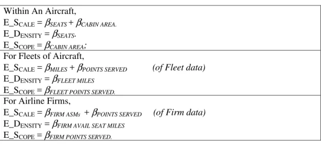
Table 2 - Cost Elasticies of Scale

Within An Aircraft,

E_SCALE = βSEATS+ βCABIN AREA.

E_DENSITY = βSEATS.

E_SCOPE = βCABIN AREA;

For Fleets of Aircraft,

E_SCALE = βMILES + βPOINTS SERVED (of Fleet data)

E_DENSITY = βFLEET MILES

E_SCOPE = βFLEET POINTS SERVED.

For Airline Firms,

E_SCALE = βFIRM ASMs + βPOINTS SERVED (of Firm data)

E_DENSITY = βFIRM AVAIL SEAT MILES

E_SCOPE = βFIRM POINTS SERVED.

2.3 Model Key Point – An Effort to Model Individual Flights, through Quarterly

fleet Aggregates

The Hicks Composite Commodity Theorem states that, “if the prices of a group of goods

move in parallel, then that group of goods can be treated as a single good.” This implies that

it is desirable to model costs below the firm level. It is unlikely that firm-wide statistics will

have the same cost elasticities of operational parameters, scale, and so on, as for its

component fleets. Therefore, the firm-wide production process ought not to be treated as a

single production function. Instead, using disaggregated data at the fleet level is more

desirable. Meaningfully, equipment-specific data will ensure that the cost function does not

mis-state the fleet level cost elasticities, which could occur without warning in the context of

conventional firm-level aggregation, whose metrics are most often averaged by departure

I use typical flights which are the average departure-weighted journey for each fleet. Fleets

usually are directed to fairly narrow bands of operations, to capitalize on the relative strengths

of each aircraft type. The mean distance per flight should have low variation within these

fleets – certainly a lower variation than when attempting firm-wide analysis. By using

quarterly data, a researcher is partway to an engineering-based cost model. Operationally

similar flying should have similar costs, regardless of which particular cities are involved.

This is because the laws of physics acting upon the aircraft are uniform, airports contestable,

and a parameter for airway congestion can be included in the model.

Consider this hypothetical example in Table 3:

Table 3 - Example of Assignment-Driven Cost Efficiency Differential

Aircraft Type Seats Stage Quarterly

Departures

Quarterly Operating Cost

Cost per Available Seat Mile

A319 120 375 mi 900 $8 million $0.198

A319 120 1,500 mi 360 $9 million $0.139

This sort of data display can be used to isolate the frontier of operational feasibility. Firms

that operate in a particular way would be expected to have particular costs by virtue of their

schedule, and its interactions with other factors. The efficient frontier of production can best

be found by examining fleet-level data. The vastly different Cost per Available Seat Mile

(CASM) in the above pair could obscure the idea that both came from the same cost function.

They may be equally efficient in terms of some underlying physical model. Their schedules

largely dictate the average speed at which the fleets operate, which directly results in

“outputs” such as ASMs that a model would expect can be produced by such fleets. We must

take care that the costs are modeled realistically, noting that each fleet has a particular

operational cost frontier.

The LHS of our regression will be the total cost of a subfleet’s operations quarterly. This is

reminiscent of a micro model of individual flights, in a Morrison/Swan engineering sense, as

if the subfleet is iterating many identical average flights. Unfortunately, in the typical

heterogeneous flight schedule, this assumption of flight uniformity is a gross simplification

that is nonetheless required, since the cost data themselves are aggregates to some extent. It is

the micro flights from fleet data. Then the fleet average operational metrics could

approximate the metrics of individual flights, upon which the laws of physics are likely to

exert a role in terms of fuel and time requirements, and therefore cost.

This is a second-best method compared to actual flight modeling. We do not have data points

for each of the roughly 10 million commercial passenger flights in the USA annually. The

dataset compares fleet level data for several hundred fleets over the period 2000-2007

(comprising 2,660 usable observation points).

3. Data and Empirical Strategy

3.1 Data Overview

This project uses US DOT Form 41 data for the years 2000-2007, an eight-year panel of

operational, financial, equipment and macro environment data. This is a large data source

with high presumed reliability and completeness. Its metrics include quarterly data for each

aircraft subfleet (such as Boeing 737-300, Airbus A319, etc) for each airline included in the

sample. The sample includes most of the major players that comprise the US commercial

market, as shown in Table 4.

Table 4 - Airlines in Sample, by Category

Legacy Carriers

Alaska Continental Northwest

Aloha Delta United

American Hawaiian US Airways

America West Midwest

Major Low-Cost Carriers

AirTran JetBlue Southwest

ATA Frontier Spirit

“Regional” Airlines

(<100 Seats / aircraft)

American Eagle Pinnacle SkyWest

Comair Mesa Air Wisconsin

This sample is diverse in equipment types, fleet counts, and styles of utilization. The data

source is time series panel data with about 8000 observations, of which about 2500 are

complete. The most commonly missing variable in dataset completeness has been network

size (points served), for which certain values could not be obtained. Other values were

manually corrected or deleted by the author if obviously false. Some included erratic

numbers in connection with extremely small operational levels.

The Form 41 data source includes fleet specific direct operating costs (DC) such as pilot

wages, fuel, etc, but does not include indirect costs (IC) like advertising and headquarters

salaries. Indirect costs are only available at the aggregate corporate level (summing the fleets

for each firm.) While corporate level Total Cost data are available on Form 41 Schedule P-12,

subfleet level data must be simulated based on a linkage assuming that overhead costs (= TC

– Direct Costs) are distributed uniformly across the firm’s produced units. For now, we say

overhead costs are distributed evenly across Aircraft Miles. This allows us to have realistic

total operating costs (TC) for each fleet, in addition to the detailed operational data.

A representative data observation is described in Table 5, and the data are summarized in

Table 6.

Table 5 - A Representative Data Observation from the Sample

Airline Aircraft Type

Quarter Departures Seats Available Avg Length of Haul Seat Capacity Available Seat Miles Gallons of Fuel Crew Costs American Airlines

MD-80 Q2 2003 112,681 17,352,000 856 mi 129 12.94 Billion

260.5 Million

$150.5 Million

Table 6 - Data summary, with Arithmetic and Weighted Means

N=2660 Mean Std Dev Minimum Maximum Weighted Mean

(ASMs) FleetMi 16,249,217 16,466,421 7,944 114,559,245 31,684,496

ACPoints 34.444 24.651 2 132 43.037

ACSeats 158.019 76.622 30 430 178.210

ACCabinArea 124.168 80.460 27.195 380 143.502

ACFlightDist 1357.54 1122.62 137.49 6570.79 1605.851

ACPilotWage 481.70 348.37 2.01 9903.38 519.923

FuelPrice 36.16 12.867 18.494 70.325 36.522

CapMPrice 5293.75 2717.54 863.15 50530.4 5816.6

TechAge 14.668 8.702 1 40 15.205

FirmASMs 20355210153 14072344362 75669086 45920502143 27411965363

FirmPoints 111.67 41.00 5 163 121.12

The dataset was assembled in Microsoft Excel using raw data from the US Department of

Transportation Bureau of Transportation Statistics online sources (www.bts.gov). Panels

were merged into quarterly, fleet specific numbers for operations and direct costs of operation

from Form 41 T2, T100. Lastly, the data were fed into SAS 9.1.3 for further data

manipulation and econometrics processing.

3.2 Model Regression Variables

For both the first-order translog and translog cost models, the dependent variable was a

calculation of Total Operating Costs. This was the sum of itemized direct costs and

synthetically disaggregated indirect costs, by fleet, in 1997 dollars.

The 13 explanatory variables are:

• Fleet Aircraft Miles • Mean Flight Distance • Equipment Design Age • Fleet Network Points • Cockpit Wage • Firm Production Quantity

• Seat Capacity • Oil Price • Firm Network Size

• Cabin Area • Capital, Materials Price • Year

(Firm identity – carrier-specific fixed effects.)

Cockpit wage is included in the regressions because, as noted by Wei and Hansen (2003),

“pilots flying larger aircraft are paid more than those flying smaller aircraft, and these

‘diseconomies’ of pilot cost offset the ‘technical’ economies of aircraft size (…)” Therefore,

I explicitly itemize the cost of the pilot factor in each fleet, from the item “Pilots and

Copilots” of quarterly operational costs on Form 41. This allows us to treat pilot wages as

essentially exogenous by entering the data. This removes bias from the coefficients on

operational choices (aircraft types and statistics), removing potential bias of the estimators

that were hiding pilot wage.

Is it reasonable to treat pilot wages as an exogenous correction of the model, but aircraft least

rates as implicit? The rationale is the liquidity of aircraft, compared to the pools of airline

pilots, which are fundamentally illiquid due primarily to unionization. But aircraft cannot

unionize. From the data, similar airlines display stark wage disparities, both over time within

firms, and among firms during constant time. This persistent illiquidity of factors is presumed

A key data omission to mention again is aircraft capital costs. I seek to omit aircraft costs by

assuming that depreciation and rent parameters are economic equals.

Rent = Amortization = Economic Depreciation of Equipment. (12)

While maintenance costs are explicitly available in Form 41, the purchase, ownership

opportunity costs, or lease arrangements are not especially amenable to direct comparison.

This becomes a serious problem if equipment cost items are only partially specified in the

model, leading to problems with the adding-up restriction across many diverse firms with

different equipment procurement or repair behaviors. Confusing the bookkeeping, a firm

could try to maximize depreciation booked on such assets for tax purposes, or engage in

accounting logic that deviates from economic realities. Rent may, consequently, be a

problematic variable in our cost function. By instead focusing on operational parameters, as

in the Morrison and Swan theory, we build equipment costs into the intercept of the equation.

Or, in our case, it could form an amorphous “ready aircraft” commodity that we can build into

Capital-Materials pricing. Firm identity variables might capture any remaining special nature

of aircraft cost. This is based on the assumption of a liquid secondhand market for aircraft

and continuous operating decisions on repairs vs. replacement of new aircraft.

4. Estimation Results

The cost model implies an industry-wide cost model and, therefore, an industry-wide

production function. The industry’s cost and production data are put into a model. The

model yields estimated coefficients for the cost elasticities of various factors and styles of

production. The degree of statistical confirmation of these estimates is reflected in the

closeness of fitment of cost outcome estimation to real cost data – i.e., the R2 for the estimated

linear regressions.

By estimating a disaggregated model, the hope is that the most appropriate estimate takes

place, which represents firm costs with respect to the type of machines employed. These

machines represent, over time, variable decision-management units that might be subject to

actual decisions or variations of production based on variables (such as seats per aircraft)

elasticity – without, and then with second-order interactions – of that type of decision upon

existing fleets. Therefore, the empirical model is historically meaningful, and also has

something to say about the effects might be of actions taken by market actors. So, the model

could reasonably be used for simulation.

The restricted model is:

ln[Total Cost] =

β0 + β1ln[Fleet Aircraft Miles] + β2ln[Fleet points served] + β3[Seat Capacity] +

β4ln[Cabin Area] + β5[Mean Flight Distance] + β6[Cockpit Wage] +

β7[Oil Price] + β8[Capital-Materials Price] + β9[Design Age] + β10[Firm Quantity] +

β11[Firm Scope] + β12[Year] + βi[firm identities].

The less resricted, translog-style model is:

ln[Total Cost] =

α0+αYlnY+ βilnWi+ φilnZi

i

∑

i

∑

2δYY(lnY)

2+

1 2

i

∑

i

∑

j

∑

j

∑

ρYilnYlnWi +

i

∑

i

∑

j

∑

i

∑

Firms

∑

4.1 First-order, Restricted Specification

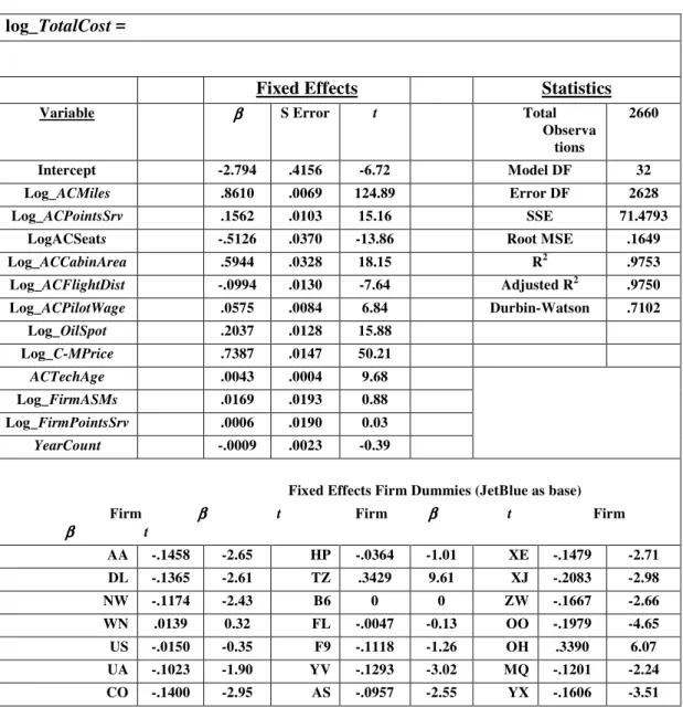
Table 7 - Subfleet First Order Total Cost Regression, 2000-2007 (1997 dollars)

log_TotalCost =

Fixed Effects Statistics

Variable ββββ S Error t Total Observa

tions

2660

Intercept -2.794 .4156 -6.72 Model DF 32

Log_ACMiles .8610 .0069 124.89 Error DF 2628

Log_ACPointsSrv .1562 .0103 15.16 SSE 71.4793

LogACSeats -.5126 .0370 -13.86 Root MSE .1649

Log_ACCabinArea .5944 .0328 18.15 R2 .9753

Log_ACFlightDist -.0994 .0130 -7.64 Adjusted R2 .9750

Log_ACPilotWage .0575 .0084 6.84 Durbin-Watson .7102

Log_OilSpot .2037 .0128 15.88

Log_C-MPrice .7387 .0147 50.21

ACTechAge .0043 .0004 9.68

Log_FirmASMs .0169 .0193 0.88

Log_FirmPointsSrv .0006 .0190 0.03

YearCount -.0009 .0023 -0.39

Fixed Effects Firm Dummies (JetBlue as base)

Firm ββββ t Firm ββββ t Firm

ββββ t

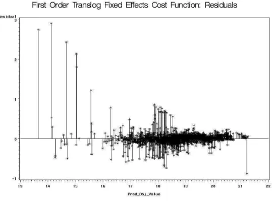
The first order translog model appears to be a good specification (according to Figure 3) and

enjoys easy interpretability. The coefficients represent fleet-level cost elasticities. Holding

all else equal, this regression allows us to interpret the economies of density and scope, cost

effects of increasing aircraft size, seat density, or oil costs and cockpit crew wages. While

prohibiting interactions among the coefficients may be a bit simplistic, this regression does

give some clear results that can be reported.

As shown in Table 8, cost elasticity of scale is approximately one (CRS is not rejected). In

practical terms, this means that a firm could expand a particular fleet with constant unit costs.

So, this means that firms have exploited available economies of scale, and attained efficient

scale. This is not unexpected, considering the contestability of markets asserted.

The cost elasticity of aircraft scale is a bit new, but also well worth examination. The

physical size of aircraft should engender greater efficiency, at least to a point. The coefficient

on cabin area suggests that total costs increase with cabin area with an elasticity of

approximately 0.594 (SE 0.33). This is so after controlling for seat count and operational

style, including length of haul. Hence, aircraft have increasing returns to scale. See Table 8

(below) for this breakdown. Returns to scale in terms of the firm are measured to be

insignificant. The coefficient on FirmASMs and FirmPointsSrv suggest that attributes of the

overall firm do not directly impact costs accrued to the fleets, which is my topic of concern.

Therefore the firm size, irrespective of fleets (which themselves have sizes), appears to carrly

little or no predictive power over costs. We might say that there are no economies, positive or

negative, associated with firm size after specifying fleet size. That’s surprising, because the

firms’ fixed costs are allocated into the fleet costs, so we would expect economies of firm size

to be visible. Also, no time trend is visible (all cost numbers are inflation-adjusted by

Figure 2 - First Order Restricted Fixed Effects: Residuals

Table 8 - Cost Elasticities of Scale and Scope12

Fixed Effects Restricted Model:

Cost Elasticities of Scale and Scope

Coeffs SE

Fleet Miles 0.861 .070

Fleet Scope 0.156 .010

⇒ Fleet Scale ⇒ 1.017 ⇒ .080

Aircraft Seats -.513 .037

Aircraft Scope .594 .033

⇒ _{Aircraft Scale}13 _⇒

0.082 ⇒ .070

12

Note: “Fleet Scale” refers to economies from more or wider operations of a given fleet; “Aircraft Scale” refers to larger or smaller aircraft.

13

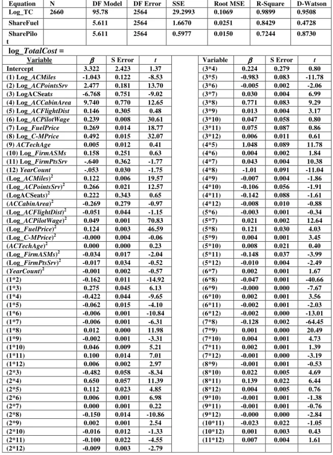
4.2 Translog Style Regression Results

Table 9 - Subfleet Translog Style Total Cost Regression, 2000-2007 (1997 dollars)

Equation N DF Model DF Error SSE Root MSE R-Square D-Watson Log_TC 2660 95.78 2564 29.2993 0.1069 0.9899 0.9508 ShareFuel 5.611 2564 1.6670 0.0251 0.8429 0.4728 SharePilo

t

5.611 2564 0.5977 0.0150 0.7244 0.8730

log_TotalCost =

Variable ββββ S Error t Variable ββββ S Error t Intercept 3.322 2.423 1.37 (3*4) 0.224 0.279 0.80 (1) Log_ACMiles -1.043 0.122 -8.53 (3*5) -0.983 0.083 -11.78 (2) Log_ACPointsSrv 2.477 0.181 13.70 (3*6) -0.005 0.002 -2.06 (3) LogACSeats -6.768 0.751 -9.02 (3*7) 0.030 0.004 6.99 (4) Log_ACCabinArea 9.740 0.770 12.65 (3*8) 0.771 0.083 9.29 (5) Log_ACFlightDist 0.146 0.305 0.48 (3*9) 0.013 0.004 3.17 (6) Log_ACPilotWage 0.239 0.008 30.61 (3*10) 0.047 0.058 0.80 (7) Log_FuelPrice 0.269 0.014 18.77 (3*11) 0.075 0.087 0.86 (8) Log_C-MPrice 0.492 0.015 32.07 (3*12) 0.006 0.011 0.61

(9) ACTechAge 0.005 0.012 0.41 (4*5) 1.048 0.089 11.78

(10) Log_FirmASMs 0.158 0.251 0.63 (4*6) 0.004 0.002 1.84 (11) Log_FirmPtsSrv -.640 0.362 -1.77 (4*7) 0.043 0.004 10.38 (12) YearCount -.053 0.030 -1.75 (4*8) -1.01 0.091 -11.04 (Log_ACMiles)2 0.122 0.006 19.57 (4*9) -0.007 0.004 -1.86

(Log_ACPointsSrv)2 0.266 0.021 12.57 (4*10) -0.106 0.056 -1.91

(LogACSeats)2 0.222 0.343 0.65 (4*11) -0.142 0.088 -1.61

(ACCabinArea)2 -0.269 0.279 -0.97 (4*12) -0.008 0.010 -0.88

(Log_ACFlightDist)2 -0.051 0.044 -1.15 (5*6) -0.003 0.001 -0.34 (Log_ACPilotWage)2 0.049 0.001 70.83 (5*7) 0.021 0.002 12.64 (Log_FuelPrice)2 0.124 0.003 46.59 (5*8) 0.121 0.030 4.03 (Log_C-MPrice)2 -0.000 0.004 -0.06 (5*9) 0.004 0.001 3.45

(ACTechAge)2 0.000 0.000 0.23 (5*10) 0.008 0.021 0.40

(Log_FirmASMs)2 -0.034 0.017 -2.04 (5*11) -0.148 0.037 -3.99 (Log_FirmPtsSrv)2 -0.017 0.034 -0.52 (5*12) -0.010 0.004 -2.49

(YearCount)2 -0.001 0.002 -0.57 (6*7) 0.002 0.001 1.67

Table 9 Continued - Subfleet Translog Style Total Cost Regression, 2000-2007

(1997 dollars)

Fixed Effects Firm Dummies

Firm ββββ t Firm ββββ t Firm ββββ t

AA 0.134 2.36 TZ 0.100 3.37 ZW -0.142 -2.38 DL 0.149 2.83 FL -0.019 -0.63 OH 0.284 5.31 US 0.141 3.90 F9 0.009 0.14 MQ -0.088 -1.49 UA 0.177 3.34 YV -0.110 -2.38 AS 0.013 0.43 CO 0.128 2.92 XE -0.108 -1.93 YX -0.175 -4.27 HP 0.034 1.19 XJ -0.422 -5.48 NW 0.116 2.54 B6 (base) 0 OO -0.224 -4.85 WN -0.096 -2.37

Figure 3 - Unrestricted Translog Style Regression: Residuals

Translog style regression results (in Table 9) can be at first difficult to interpret since

second-order effects (particularly with output) may obscure the first-second-order effects of the coefficients.

For example, the inclusion of quadratics decomposes the first order interpretability we had in

the first-order translog function. While CCT reported near-exact matches between first-order

translog and first-order coefficients from the full translog regressions, it does not occur here.

The most interesting aspects of the translog results occur in observing the sign and

positively correlated with older aircraft designs. Knowing this can lead to more realistic

analysis and simulation.

The interaction of output (AC Miles) with inputs or characteristics also yielded interesting

information. For bigger fleet outputs, the cost efficiency has been improving over time. With

a coefficient of .006 (.002), as each year will have passed, growth of AC Miles will have had

had a cost elasticity closer to unity. The cost economy available from growing a fleet has

diminished over time.

4.3 Returns to Scope, Scale

4.3.1 Fleets

The initial first-order translog total cost model suggests that fleets have constant returns to

fleet scale (AircraftMi), with cost elasticity of density (SE) of 0.861 (.007), and cost elasticity

of fleet network size [scope] .156 (.010). Cost elasticity of total scale may be unity, and CRS

cannot be rejected. The interpretation is, it appears that most firms operate their fleet at sizes

large enough that further cost economies of scale are beyond reach.

As expected, the coefficient on mean Flight Distance is negative; as a flight distance doubles,

costs will fall by 7.6%. This is because Aircraft Miles have remained fixed, and as such,

longer flights will be cheaper, with fewer departures, higher average speeds, and better

productivity, as this model understands it.

Evidently, costs also increase with the design age of the fleets. Total costs rise by 0.43% (SE

.0004) for each year older an aircraft fleet’s mechanical design may be (these data were

compiled by the author). The YearCount dummy (measuring annual changes in cost

efficiency) is insignificant in itself in the TL style model, ignoring the issue of fleet design

aging.

4.3.2 Firms

In the context of the fleet costs, the model does question whether firm total output quantity

(ASMs) or firm geographic scope (PointsSrv, for the whole company) affect fleet costs. It

The economy of scope (additional airports served) suggests it is quite cheap for firms to

expand a given fleet’s geographical “footprint,” with an elasticity of only 0.156 (SE .01) for

adding new network points while maintaining service quantity. This suggests an existing fleet

could serve an additional city, or group of cities, rather cheaply. This, in turn, aids the

argument that the overall market is contestable.

4.3.3 Aircraft

With respect to physical aircraft size, IRS are seen. The coefficient on ACCabinArea

suggests that as we double aircraft interior space, costs rise by 59%. This suggests positive

economies of scale.

While the coefficient on ACSeats appears to suggest more seats result in actual cheaper

flying, this is only an artifact of the context of fixed cabin size. This is probably because

higher density seating configurations may be correlated with generally lower-cost firms,

somehow missed despite our control for firm identities. Correspondingly, if a fleet within a

firm were higher density, there may be unobserved traits about such a fleet that make it

cheaper to operate (perhaps being an experimental subsidiary airline such as Metrojet, Song

or TED, whose operations are included in this study under their corporate parents). This

might explain, in part, why we see costs apparently falling as seat counts rise. An alternative

model, with seating density in place of count, also produced this.

4.4 Energy Cost Share and Response to Perturbation

The sum of cost shares of Pilot Wages, Oil and Capital-Materials were constrained to unity in

the regression using SUR in PROC SYSLIN (for the restricted model), and later in PROC

MODEL (for the full TL style model). Their computed cost shares are 5.8%, 20.4% and

73.9% respectively. It should be noted again that the first-order translog functional form does

not allow these cost shares to vary across the diversity of our sample, or even across time. A

more flexible cost function specification allow them to move within their constraints.

The unrestricted translog style results show that energy cost share varies negatively with

output scope and density; negatively with cabin area; and positively with flight distance. This

In an unexpected energy shock, the returns to “green technology” rise would more steeply

than anticipated, providing a windfall for those who invested in efficient machinery vs. their

own forecasts. Conversely, those with the oldest technology will face an unexpected

competitive problem. Typically, in a clearing market with risk neutral entities, we would

expect that:

Σ(costs new / green technology) = Σ(costs of old technology); (13)

E[marginal rent on new aircraft] = E[added fuel cost in old aircraft].

Yet, we can see from our translog style results that apparently old machinery does not unduly

penalize their operators. As oil prices rise, the coefficient on the interaction between log (Oil

Price) and Tech Age was not significant in this study. Total costs of the airline are not

exacerbated by the presence of older equipment, or minimized by the use of new equipment.

Unexpected shifts in fuel cost seem to maintain the pure cost equivalence I assumed between

new and old aircraft. However, it is worth remembering that older aircraft are more costly to

run, according to the unrestricted model’s TechAge coefficient.

The movements of oil prices are exogenous to the airline industry. But rolling expectations of

oil prices may guide fleet procurement. From the data and the cost function measured here,

we can describe what total costs would have been for the sample group of firms, between

2000-2007, at various fuel prices. This does not include feasibility conditions or capacity

readjustments. A trend toward energy efficiency can be seen, as, although output has

remained relatively constant, fuel burn has fallen and, hence, the industry is more robust to an

oil price spike in 2007 than it was in 2000. The cost function is undefined at oil price = $0,

which is why the curve appears to join the origin. This graphic (Fig. 4) uses the translog style

cost function from this project to extrapolate various costs for each observation in the data.

The projected costs are then summed across the industry to get a total.

Similar to literature such as Thompson (2006), we can find energy cost share by Shephard’s

Lemma: