SYNTHESIS OF AN LMI-BASED FUZZY CONTROL SYSTEM WITH
GUARANTEED COST PERFORMANCE: A PIECEWISE LYAPUNOV
APPROACH
Natache S. D. Arrifano
∗ [email protected]Vilma A. Oliveira
∗ [email protected]L ´ucia V. Cossi
† [email protected]∗Departamento de Engenharia El´etrica, Universidade de S˜ao Paulo
Av. Trabalhador S˜ao Carlense, 400 CEP 13566-590, S˜ao Carlos, SP, BRASIL
†Departamento de Matem´atica, Universidade Federal da Para´ıba
Cx. Postal 5080
CEP 58051-970, Jo˜ao Pessoa, PB, BRASIL
ABSTRACT
A new stability analysis and design of a fuzzy switching control based on uncertain Takagi-Sugeno fuzzy systems are proposed. The fuzzy system adopted is composed by a fam-ily of local linear uncertain systems with aggregation. The control design proposed uses local state feedback gains ob-tained from an optimization problem with guaranteed cost performance formulated in the context of linear matrix in-equalities and a fuzzy switching scheme built from local Lya-punov functions. The global stability is guaranteed by con-sidering a class of piecewise quadratic Lyapunov functions. Examples are given to illustrate the applicability of the pro-posed approach.
KEYWORDS: Switching fuzzy control, Guaranteed cost
fuzzy control, Uncertain Takagi-Sugeno fuzzy systems, Piecewise quadratic Lyapunov functions.
Artigo submetido em 28/11/2002 1a. Revis ˜ao em 26/06/2003 2a. Revis ˜ao em 18/03/2004 3a. Revis ˜ao em 29/05/2006
Aceito sob recomendac¸ ˜ao do Editor Associado Prof. Cairo Lucio Nascimento Jr
RESUMO
Neste trabalho, uma nova an´alise de estabilidade e projeto de controle fuzzy chaveado baseado em sistemas fuzzy Takagi-Sugeno com incertezas s˜ao propostos. O sistema fuzzy ado-tado ´e composto por uma fam´ılia de sistemas lineares in-certos locais com agregac¸˜ao fuzzy. O projeto de controle proposto utiliza ganhos de realimentac¸˜ao de estado locais obtidos da soluc¸˜ao de um problema de otimizac¸˜ao com sempenho de custo garantido formulado em termos de de-sigualdades matriciais lineares e um esquema de chavea-mento fuzzy baseado em func¸˜oes de Lyapunov, que s˜ao usa-das quando a trajet´oria do estado do sistema est´a na fronteira de subespac¸os definidos do espac¸o de estado. A estabili-dade global ´e garantida considerando uma classe de func¸˜oes de Lyapunov quadr´aticas por partes. Exemplos ilustram a aplicac¸˜ao da abordagem proposta.
PALAVRAS-CHAVE: Controle fuzzy chaveado, Controle
1
INTRODUCTION
Takagi-Sugeno (TS) fuzzy-model-based control has been successful used to control nonlinear systems in several ap-plications (Tanaka et al., 1999; Feng et al., 1997; Wang et al., 1996). Most of the techniques of robust control have been used in the TS fuzzy-model-based control due to the fact that the TS fuzzy systems can be interpreted as differential inclusions (Jadbabaie et al., 1998a; Cao et al., 1997; Tanaka et al., 1996). However, when treating uncer-tain nonlinear systems, we need to distinguish nonlinear-ity from uncertainty, otherwise, the results obtained are in general conservatives. Several approaches have appeared to the robust stabilization of uncertain nonlinear systems (Lee et al., 2001; Cao et al., 2001; Teixeira and ˙Zak, 1999; Tanaka et al., 1996). In the framework of TS fuzzy systems, paramet-ric uncertainty can be represented by norm-bounded or poly-topic uncertain sets. Different robust control solutions for the TS fuzzy system with norm-bounded and polytopic un-certainty representations can be found in Tanaka et al. (1996) and Lee et al. (2001), and Cao et al. (2001), respectively.
Stability is one of the most important issues when analyzing control systems. Most of the methods of fuzzy-model-based control yields stability analysis and design procedures by means of the parallel distributed compensation (PDC) using a common quadratic Lyapunov function (Teixeira et al., 2000; Tanaka et al., 1998; Tanaka et al., 1997). This approach requires a common positive definite matrix that is a solu-tion of all the Lyapunov inequalities built from the local lin-ear systems of the global feedback TS fuzzy system, which are usually formulated in terms of linear matrix inequalities (LMI’s) in both the state feedback gain and Lyapunov matrix. However, when applied to uncertain nonlinear systems, this approach may not provide feasible results because it is not possible to find a common positive definite Lyapunov ma-trix as a solution of several Lyapunov inequalities. To re-move this deficiency, recently, attractive stability results for the TS fuzzy-model-based control using piecewise quadratic Lyapunov functions appeared (Zhang et al., 2001; Johansson et al., 1998). These results explore the gain-scheduled na-ture of the fuzzy controllers and have found application in the stability analysis of systems whose dynamics depends on the subspace of the state space their trajectory is.
This paper presents a fuzzy switching controller for uncer-tain nonlinear systems which are represented by a class of TS fuzzy systems with uncertainties. The controller pro-posed uses local guaranteed cost control laws and a switching scheme based on local quadratic Lyapunov functions when the state is on the boundary of defined subspaces of the state space. A sufficient condition for the stability of the uncertain nonlinear system with state feedback is given in terms of a piecewise quadratic Lyapunov function. This approach
pro-duces less conservative results than those obtained with the fuzzy blending controller for TS fuzzy systems with uncer-tainties. In addition, this approach may be applied to con-trol highly nonlinear systems, where available robust concon-trol techniques are not successful.
The remainder of the paper is organized as follows. In Sec-tion 2, the fuzzy system modeling for a class of uncertain nonlinear systems, the fuzzy switching control and the guar-anteed cost control design are presented. The stability anal-ysis of the feedback fuzzy system is the subject of the Sec-tion 3. In SecSec-tion 4, simulaSec-tion results are presented to illus-trate the effectiveness of the proposed approach. Finally, the paper concludes with brief remarks in Section 5.
2
FUZZY SYSTEM MODELING AND
CON-TROL
We consider a class of uncertain nonlinear dynamic systems which are described by the differential inclusion
˙
x∈Co{fk(x) +gk(x)u}, x(0) =x0, (1)
wherexis the system state vector,uis the input vector,Co
denotes the convex hull, fk(·), gk(·) are smooth nonlinear functions which define the called vertex systems,fk(0) = 0,
gk(0) = 0, andv is the number of vertexes,k = 1,2, ..., v, with fk : Rn → Rn and gk : Rn → F(Rm,Rn) for F(Rm,Rn) ={h:D(h)→Rn:D(h)⊆Rm.
Considering an uncertain parameter vectorp ∈ Rs, a poly-topic representation of (1) has the form
˙
x=
v
X
k=1
ηk(p)(fk(x) +gk(x)u), (2)
where ηk : Rs → R with ηk(p) ≥ 0, k = 1,2, ..., v,
Pv
k=1ηk(p) = 1.
2.1
Fuzzy system modeling
rule is given by
Rulei:
Ifx1isF1iandx2isF2iand . . .xnisFni
Thenx˙ =Ai(p)x+Bi(p)u
i= 1,2, . . . , r, (3)
whereFi
j,j = 1,2, . . . , nare fuzzy sets, r is the number
of inference rules, and matricesAi(p) ∈ M(Rn,Rn)and
Bi(p))∈ M(Rn,Rm)have a polytopic representation, that is,Ai(p) =Pkv=1ηk(p)Aik andBi(p) = Pvk=1ηk(p)Bik, forηk(p) ≥ 0,k = 1,2, ..., v,Pvk=1ηk(p) = 1. Matrices
Ai(p)andBi(p), i = 1,2, . . . , rcan be obtained from (2) using the linearization formula proposed by Teixeira and ˙Zak (1999), which yields a good linear approximation of nonlin-ear systems in the vicinity of an operating point even if it is not an equilibrium point. The Teixeira & ˙Zak linearization formula used in this paper is presented in Appendix A.
Given the pair(x, u), the overall fuzzy system with uncer-tainties is inferred as a weighted average of all local uncertain linear approximations(Ai(p), Bi(p)),i= 1,2, . . . , rof (3), which is given by
˙
x=
r
X
i=1
αi(x)(Ai(p)x+Bi(p)u), (4)
where
αi(x) =
Qn
j=1Fji(xj)
Pr
i=1
Qn
j=1Fji(xj)
(5)
denotes the normalized membership function, withFi j(xj)∈
[0,1]the grade of membership ofxj,j = 1,2, . . . , n, in the fuzzy setFi
j. Considering the fact that in (5)Fji(xj) ≥ 0,
i= 1,2, . . . , randj = 1,2, . . . , n, we haveαi(x)≥0and
Pr
i=1αi(x) = 1,∀t≥0.
2.2
Fuzzy switching control
In this section we propose a switching scheme so that local controllers are switched according to the subspace that the state vectorxenters. For this purpose, letS◦
i denote theith subspace in the state space
S◦
i :={x|αi(x)> αℓ(x);i6=ℓ;i, ℓ= 1,2, . . . , r}, (6)
where the superscript◦ inS
idenotes an open subspace, let
∂Siℓdenote the transition subspace in the state space
∂Siℓ:={x|αi(x) =αℓ(x);i6=ℓ;i, ℓ= 1,2, . . . , r}, (7)
and letSi = Soi
S∂S
iℓ. Using (6) and (7), we define the switching scheme for each rulei
Rulei:
If x∈S◦
i Then βi(x) = 1
If x∈∂SiℓandVi(x)≤Vℓ(x) Then βi(x) = 1andβℓ(x) = 0
i6=ℓ, i, ℓ= 1,2, . . . , r, (8)
whereVi(x) = xTPixis a local quadratic Lyapunov func-tion, withPi=PiT,Pi>0andβi(x)∈ {0,1}a crisp func-tion which changes asxleaves subspaceS◦
i following the membership function changes. Thus,βi(x) = 1only when
x∈Si=Si◦∪∂Siℓandβi(x) = 0, otherwise. Additionally,
Pr
i=1βi(x) = 1,∀t≥0.
Adopting (8) and following the idea of the PDC scheme, we propose the fuzzy switching control as
u=−
r
X
i=1
βi(x)Kix, (9)
whereKi ∈ M(Rm,Rn),i= 1,2, . . . , rare the state feed-back gains to be designed for rulei. In order to obtain the state feedback fuzzy system, we substitute (9) in (4), which gives
˙
x =
r
X
i=1
αi(x)
Ai(p)−
r
X
j=1
βj(x)Bi(p)Kj
x
r
X
i=1 r
X
j=1
αi(x)βj(x) (Ai(p)−Bi(p)Kj)x. (10)
Recalling that from (8)βi(x) = 1only whenx∈Si, we can write (10) as
˙
x=
r
X
i=1
αi(x)(Ai(p)−Bi(p)Ki)x. (11)
The state feedback fuzzy system (11) is recognized as an ag-gregation ofrlocal feedback uncertain systems described in a polytopic form.
2.2.1 Guaranteed cost control design
Definition 1 The ith feedback uncertain linear system of (11) is said to be asymptotically stable, if there exists a stabi-lizing controlu=−Kix,i= 1,2, . . . , r, such that an upper bound on the quadratic performance index
Ci(x0, u) =
Z ∞
0
(xTQix+uTRiu)dt, x0∈Si◦, (12)
along the system trajectory is minimized, withQi ∈Rn×n,
Ri ∈ Rm×m, Qi > 0, andRi > 0 weighting symmetric matrices which are chosen to yield the desired performance.
Definition 2 If there exist a stabilizing control law u =
−Kix,i = 1,2, . . . , r and a positive scalarCˆi, such that,
Ci(x0, u) ≤ Cˆi along the system trajectory, then Cˆi is a guaranteed cost anduis a guaranteed control law.
Proposition 1 Consider theith uncertain linear system of (4), control lawu = −Kix, i = 1,2, . . . , r and cost per-formance (12). If there exist symmetric positive definite ma-tricesXiand matricesYi,i = 1,2, . . . , rof appropriate di-mensions satisfying the LMI’s
Qi>0, Ri>0, Xi>0,
Uik Zi
ZT
i −W
<0,
∀i= 1,2, . . . , r;k= 1,2, . . . , v, (13)
where
Uik = XiATik+AikXi−YiTBikT −BikYi,
Zi=
h
XiQ1i/2 YiTR 1/2 i
i
,
W = diag
In, Im ,
Xi= Pi−1,
Yi= KiXi,
then u = −Kix, with Ki = YiXi−1, i = 1,2, . . . , r is a guaranteed control law and the cost given by Cˆi =
xT
0Xi−1x0 is a guaranteed cost for the ith feedback uncer-tain system of (11).
Proof: Consider a local quadratic Lyapunov function
candi-date as
Vi(x) =xTPix, (14)
which is a continuous-time function along the trajectory of (11) in the subspaceS◦
i. Taking its derivatives, it results
˙
Vi(x) = x˙TPix+xTPix,˙
= xTnα i(x)
h
(Ai(p)−Bi(p)Ki)TPi
+Pi(Ai(p)−Bi(p)Ki)]}x,
= xT
( v X
k=1
αi(x)ηk(p)
h
(Aik−BikKi)TPi
+Pi(Aik−BikKi)]}x. (15)
Now assume that there exist symmetric positive definite ma-trices Pi = Xi−1 and matrices Ki = YiXi−1 satisfying LMI’s in (13). Then, using the Schur complement (Boyd et al., 1994) after performing some algebraic manipulations, (13) can be reduced to
(Aik−BikKi)TPi+Pi(Aik−BikKi)
+Qi+KiTRiKi<0,
i= 1,2, . . . , r, k= 1,2, . . . , v. (16)
UsingPv
k=1ηk(p) = 1, after some algebraic manipulations, (16) can be written as
v
X
k=1
ηk(p)
h
(Aik−BikKi)TPi+Pi(Aik−BikKi)
i
+Qi+KiTRiKi<0,
i= 1,2, . . . , r. (17)
Using (17) in (15), as αi(x) ≥ 0, we have V˙i(x) < 0, ∀x 6= 0,x ∈ S◦
i. Now, substituting (9) in (12) and using the fact thatβi(x)βj(x) = 0,i 6= j, i, j = 1,2, . . . , rand
βi(x)βi(x) = 1, forx∈Si◦it results
Ci(x0, u) <
Z ∞
0
xT(Q
i+KiTRiKi)x dt
<
Z ∞
0
˙
Vi(x)dt
= xT0Pix0. (18)
The results then follows by Definitions 1 and 2. ✷
The optimal quadratic guaranteed cost control problem in-volves the minimization of the cost bounds given by Cˆi =
xT
0Pix0, i = 1,2, . . . , rwhich depends on the initial
con-dition x0 ∈ Si◦. To remove this dependence on x0 one may assume it is a zero mean random variable satisfying
E[xT
0x0] = 1and consider the minimization ofT r(Pi)as
E[Ci]≤E[xT0x0] =T r(Pi), withE[·]the expectancy oper-ator andT r(·)is the trace (Jadbabaie et al., 1998b; Petersen and Macfarlane, 1994). Instead, we construct an optimiza-tion problem for the guaranteed cost control by minimizing an upper bound on the guaranteed costCˆi.
Lemma 1 IfCˆi is a guaranteed cost for theith state
feed-back uncertain linear system of (11) under performance in-dex (12) then forx0∈S◦i
ˆ
CBi=λmax[Xi−1]kx0k2, (19)
i= 1,2, . . . , r, is a guaranteed cost for theith state feedback uncertain linear system of (11) and an upper bound for (12), withλmax[·]the maximum eigenvalue andk·kthe Euclidean
Proof: Using singular value decompositions the result
fol-lows straightforward. ✷
Using both Proposition 1 and Lemma 1, we can construct the generalized eigenvalue problem (GEVP) (Boyd et al., 1994) for the guaranteed cost control design as
min
Xi,Yi
γisubject toIn ≤γiXiand(13). (20)
If (20) is feasible, we have γi > λmax[Xi−1] and Ki =
YiXi−1,i= 1,2, . . . , r.
3
STABILITY ANALYSIS
In Section 2 an approach to obtain the feedback gains and the quadratic Lyapunov functions associated is presented. Now, we establish a condition for the global stability of the feed-back fuzzy system (11) by considering a class of piecewise quadratic Lyapunov functions and the fuzzy switching con-trol proposed.
Theorem 2 The equilibriumx= 0of the global feedback TS fuzzy system with uncertainties (11) is asymptotically stable in the large if each uncertain linear system of (4) is locally stabilizable by the fuzzy switching controller (9) withβi(·)
as defined in (8) andKi resulting from (20), which is time
continuous in the open subspaceS◦
i.
Proof: Let
V(x) =
r
X
i=1
βi(x)Vi(x) (21)
be a piecewise quadratic Lyapunov function candidate with
Vi(x)as in (14) andPi =Xi−1,Xiresulting from (20) for each subspace S◦
i of the state space. In order to evaluate the derivative of (21) along the system trajectory, we replace
˙
V(·)by the Dini derivativeD∗V(·), where the superscript∗
inDV(·)represents any of the four Dini derivatives (Rouche et al., 1977). At any point whereV˙(·)exists, all four Dini derivatives have a common value equal to the derivativeV˙(·)
at that point. See Apendix B for more details on the Dini derivatives. Let us consider the stability at the switching time. In the sequence, we usex(t)to emphasize the anal-ysis.
Suppose that for some particular time t, x(t) ∈ S◦
i which yieldsβi(x(t)) = 1using (8). Also, suppose that the sys-tem equilibriumx(t) = 0does not exclusively belong toS◦
i, otherwise there might be no switching of controllers. Af-ter a period of time, a switching occurs, say att = t1, and
x(t)leaves the subspaceS◦
i and enters theℓth subspaceSℓ◦. We can thus writelimt→t−
1 βi(x(t)) = βi(x(t1)) = 1and
limt→t+
1 βℓ(x(t)) =βℓ(x(t1)) = 1
. The corresponding up-per and lower Dini derivatives of (21) in the transition region
∂Siℓare thus as
D+V(x(t1)) =D+V(x(t1)) = lim
ǫ→0+
0< t−t1≤ǫ
sup
1
t−t1 r
X
ℓ=1
[βℓ(x(t))Vℓ(x(t))−βℓ(x(t1))Vℓ(x(t1))],
(22)
D−V(x(t
1)) =D−V(x(t1)) = lim
ǫ→0−
ǫ≤t−t1<0
sup
1
t−t1 r
X
i=1
[βi(x(t))Vi(x(t))−βi(x(t1))Vi(x(t1))].
(23)
To haveV(·)decreasing along the system trajectory any of the four Dini derivatives must be negative definite on the open subspaceS◦
i (see Corollary 7 in Appendix B). By the switching scheme (8),D+V(·)in (22) is equal toV˙
ℓ(·)which is negative definite asx∈S◦
ℓ. Then, asβi(·)is a crisp func-tion associated to each subspaceS◦
i,i= 1,2, . . . , r, we can write
D+V(x(t)) =
r
X
i=1
βi(x) ˙Vi(x)
=
r
X
i=1
βi(x)[ ˙xTPix+xTPix˙]. (24)
Now, using (11) we can write (24) as
D+V(x(t)) =
r
X
i=1
βi(x)xT
( r X
i=1 v
X
k=1
αi(x)ηk(p)
[(Aik−BikKi)TPi+Pi(Aik−BikKi)] x, (25)
withKi=YiXi−1,XiandYi,i= 1,2, . . . , rresulting from (20). Using the proof of Proposition 1, forβi(·)given by (8) we haveD+V(x)<0,∀x,x6= 0, which assures that system (11) is stable.
We proceed with the proof showing the stability in the large. Let us define
−Nik := (Aik−BikKi)TPi+Pi(Aik−BikKi), (26)
where Nik = NikT, Nik > 0. For x ∈ Si◦, x 6= 0,
i= 1,2, . . . , r, we haveV˙i(x)<−ρVi(x)whereρis a posi-tive number defined byρ := min
i {λmin[Nik]/λmax[Pi]},
eigenvalues, respectively. By the well-known Gronwall-Bellman lemma (Khalil, 1996) we can show that forx0∈Si◦,
Vi(x)≤Vi(x0)e−ρt. Thus, from (24), it follows that
D+V(x(t)) =
r
X
i=1
βi(x) ˙Vi(x)
≤ −ρ
r
X
i=1
βi(x)Vi(x)
≤ −ρ
r
X
i=1
βi(x0)Vi(x0)e−ρt
= −ρV(x0)e−ρt (27)
asβi(·)is a crisp function associated to each subspaceSi◦,
i= 1,2, . . . , r, which completes the proof. ✷
Remark 1 In order to compare the results given, we include
in Appendix C, a fuzzy blending control approach which is also formulated as an optimal quadratic guaranteed cost control problem but adopting a common quadratic Lyapunov function (Arrifano and Oliveira, 2002).
Remark 2 To consider the stability of an uncertain
nonlin-ear system for the case the originx = 0is not the equilib-rium, one should perform a change of coordinates to make it the equilibrium, before designing the fuzzy switching control (9) withβi(·)as defined in (8). This change of coordinates is important because real systems, in general, have equilib-rium different from the origin and the control design pro-posed considers asymptotic stability around the equilibrium
x= 0.
4
SIMULATION RESULTS
In this section, the usefulness of the switching fuzzy control is illustrated. We consider the stabilization of a magnetic sus-pension system and a mass-spring-damper system using the optimal quadratic guaranteed cost control. A feasible solu-tion for the latter system can be obtained with the blending fuzzy control by means of a common Lyapunov function (see Appendix C) but no feasible solution is found for the former system.
Example 3 Nonlinear magnetic suspension system. We consider the same example as in Costa and Oliveira (1999), a nonlinear magnetic suspension system depicted by
˙
xr1= xr2
˙
xr2= g−
Lbo(xr1)
2am
xr3
1+(xr1)/a
2
˙
xr3= −
Rb
Lb
xr3+
1 Lb
ur,
(28)
Table 1: Magnetic suspension system parameters.
g M Rb Lb Lb0 a
9.81 2.26×10⁻² 19.91 470 0.0245 6.07×10⁻³
wherexr1is the ball vertical position [m],xr2is the ball ver-tical speed [m/s],xr3is the coil current [A],uris the coil ap-plied voltage [V],gis the acceleration due to gravity [m/s2],
mis the ball mass [Kg],Lbis the coil inductance [H],Rbis the coil resistance [Ω],ais a constant [m], andLb0expresses the relationship between the inductance and the ball vertical position [H]. Table 1 shows the numerical values of phys-ical parameters. Note that the equilibrium of (28)(xe, ue) is not the origin. As mentioned in Remark 2, it is neces-sary to perform a change of coordinates to bring the equilib-rium of the system to the origin. For this purpose, we adopt
z =xr−xeandv =u−ue, withxe = [0.010 0 0.8775] andue= 17.4621the equilibrium of (28). Using these new coordinates, we may write (28) as
˙
z1= z2+xe2
˙
z2= g−
L
b0(z1+xe1)
2am
z3+xe3
1+(z1+xe1)/a
2
˙
z3= −
Rb
Lb
(z3+xe3) +
1 Lb
(v+ue).
(29)
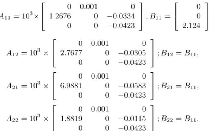
The uncertain linear systems are obtained using the lineariza-tion formula given in Appendix A considering Lb0 as the uncertain parameter with deviations of about ±80%from its nominal value. Adopting r = 2 as the number of lin-earization points chosen andx¯(r=1)= [0.005 0 0.6045]and
0 0.002 0.004 0.006 0.008 0.01 0.012 0.014 0.016 0.018 0.02 0
0.2 0.4 0.6 0.8 1
x
r1(t) [m]
0 0.2 0.4 0.6 0.8 1 1.2 1.4 1.6 1.8 0
0.2 0.4 0.6 0.8 1
xr3(t) [A]
Subspace S1 Subspace S
2
Subspace S2 Subspace S1
Figure 1: Membership functions adopted with “-” theF1 j(xj) and “· · ·”F2
¯
x(r=2) = [0.015 0 1.1505]as the linearization points, we found the matrices representing the extreme linearized sys-tems of each vertex system as
A11= 10
3
× 2
4
0 0.001 0
1.2676 0 −0.0334
0 0 −0.0423
3
5, B11=
2
4
0 0 2.124
3
5,
A12= 10
3
× 2
4
0 0.001 0
2.7677 0 −0.0305
0 0 −0.0423
3
5;B12=B11,
A21= 10
3
× 2
4
0 0.001 0
6.9881 0 −0.0583
0 0 −0.0423
3
5;B21=B11,
A22= 10
3
× 2
4
0 0.001 0
1.8819 0 −0.0115
0 0 −0.0423
3
5;B22=B11.
Figure 1 shows the membership functions adopted forxr1∈
[0, 0.020]andxr3 ∈ [0, 1.5]. Following, we present sim-ulation results which are organized in two cases: (Case 1) Lb0(xr1) = Lb0 as in Costa and Oliveira (1999) and (Case 2) Lb0(xr1) = Lb0(0.85 + 0.5/(1 + xr1/a)), with
Lb0 = 0.0245H, the nominal value for Lb0(·). The pro-posed approach is systematically accomplished by using the Matlab LMI solver as well as the ordinary differential equa-tion (ODE) solver. We adopt the initial condiequa-tion as x0 =
[0.005 0 0.6045].
In Case 1 we adopt the weighting matrices
Qi=
2
4
106 0 0
0 1 0
0 0 1
3
5andRi= 0.05,fori= 1,2
as in Costa and Oliveira (1999). In Case 2 we adopt the weighting matrices
Q1=
2
4
105 0 0
0 1 0
0 0 1
3
5;Q2=
2
4
5×10⁴ 0 0
0 1 0
0 0 1
3
5;
R1= 0.001andR2= 0.05.
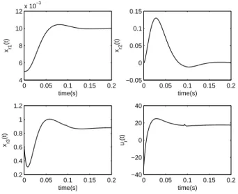
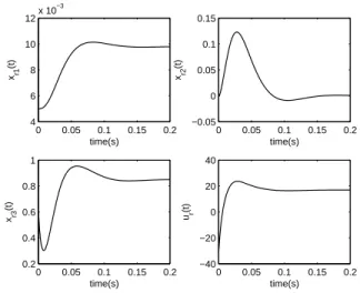
The numerical results are summarized in Table 2 and 3 for Cases 1 and 2, respectively. Figures 2 and 3 show the re-sponses of system (28) for Case 1 and Figures 4 and 5 present the responses for Case 2. Using the fuzzy switching control approach, the switching in the control law can be flattered by adjusting the width and the type of the membership functions adopted as well as the matricesQiandRi,i = 1,2, . . . , r. Therefore, the proposed solution can yield smother solutions than the one given in Costa and Oliveira (1999) using attrac-tion domains for the switching control scheme. Other charac-teristic of this approach is that the switching is related to the smaller value of the associated Lyapunov function when the
Table 2: (Case 1) Numerical results of the control design.
SubspaceS1
K1= 104× −1.4059 −0.0271 0.0080
xT
0P1x0= ˆC1= 9.103×10⁻¹ Upper bound:CB1= 3.2452×10⁴
SubspaceS2
K2= 104×
−4.1134 −0.0700 0.0181
xT
0P2x0= ˆC2= 2.9634 Upper bound:CB2= 1.0585×10⁵
Table 3: (Case 2) Numerical results of the control design.
SubspaceS1
K1= 104×[−2.1864 −0.0388 0.0100]
xT
0P1x0= ˆC1= 7.15×10⁻² Upper bound:CB1= 1.7002×10³
SubspaceS2
K2= 104×[−3.5301 −0.0608 0.0167]
xT
0P2x0= ˆC2= 1.5781 Upper bound:CB2= 7.5344×10³
state is on the boundary of the defined subspaces, but the sys-tem solution always returns to the subspace that better repre-sents the dynamics of the nonlinear system. After the state vector enters the subspace where the equilibrium pointxe is, the switching occurs if the resulting Lyapunov functions have not reached the origin or if the system are subjected to perturbations.
Example 4 Nonlinear mass-spring-damper system. We
con-sider now the same example as in Tanaka et al. (1996), a nonlinear mass-spring-damper system with an uncertain pa-rameter, which is described as
My¨+g(y,y˙) +f(y) =φ( ˙y)u, (30)
whereM is the mass [Kg],uis the force [N],yis the verti-cal position [m],y˙is the speed [m/s],g(y,y˙) = c1y+c2y˙,
f(y) = c, and φ( ˙y) = 1 +c5y˙3 are the nonlinear or un-certain terms with respect to the spring, the damper and the input system, respectively. The control purpose is to achieve the equilibrium(x, u) = (0,0)with the minimization of an upper bound on the guaranteed cost. Considering the param-eters M = 1, c ∈ [c3, c4], c1 = 0,c2 = 1, c3 = 0.5,
c4= 1.81andc5= 0.13, and definingx:= [y y˙]T, we can write (30) in the state space representation
˙
x1
˙
x2
=
−1 −c
1 0
x1
x2
+
1 + 0.13x3 1
0
u.
0 0.05 0.1 0.15 0.2 4
6 8 10
12x 10
−3
xr1
(t)
time(s)
0 0.05 0.1 0.15 0.2
−0.05 0 0.05 0.1 0.15
xr2
(t)
time(s)
0 0.05 0.1 0.15 0.2
0.2 0.4 0.6 0.8 1 1.2
xr3
(t)
time(s)
0 0.05 0.1 0.15 0.2
−40 −20 0 20 40
ur
(t)
time(s)
Figure 2: (Case 1) Magnetic suspension system statexrand controlu.
As system (31) presents one uncertain parameter, we have two vertexes in the polytopic description. We adoptr = 2
and again we obtain the uncertain linear systems using the linearization formula for the following linearization pointsx¯:
¯
x(r=1) = [1.9740 0]T andx¯(r=2)= [−1.9740 0]T, which gives
A11 =
»
−1 −0.5
1 0
–
, B11=
»
1.4387 0
– ,
A12 =
»
−1 −1.81
1 0
–
, B12=B11,
A21 = A11, B21=
»
0.5613 0
– ,
A22 = A12, B22=B21.
The performance of the proposed approach can be verified adoptingα1(x) = 0.5 +x31/6.75,α2(x) = 0.5−x31/6.75 andc= 1.155 + 0.655 cos(3x10 sin(x1)
2 )forx1∈[−1.5, 1.5] andx2 ∈ [−1.5, 1.5]. The control design is systematically developed by solving the optimization problem (50). We chooseQ = I2 andR = 0.07 for both rules and adopt initial conditionx0 = [−0.5 −1.0]T. Using the Matlab LMI solver, we obtain the main results summarized in Table 4. Figure 6 shows the feedback uncertain nonlinear system responses. The proposed approach is comparable to the one given in Tanaka et al. (1996). Its advantage is that it follows a systematic procedure and minimizes an upper bound on the quadratic performance cost.
5
CONCLUSION
In this paper we propose a fuzzy switching control design to stabilize a class of uncertain nonlinear systems represented
0 0.05 0.1 0.15 0.2 0
1 2 3 4 5
t[s] 0.085 0.09 0.095 0.1 0.105 0
1 2 3 4 5x 10
−3
0 0.05 0.1 0.15 0.2 −10
−5 0 5
t[s] 0.085 0.09 0.095 0.1 0.105 −0.1
0 0.1 0.2 0.3 0.4
Switching instant
Switching instant V
1(t)
V
2(t)
V(t)
dV
1/dt
dV
2/dt
dV/dt
Figure 3: (Case 1) Lyapunov functions and their derivatives along the system trajectory.
Table 4: Numerical results of the control design.
K1= [1.60 1.08]
K2= [4.10 2.77]
xT
0P x0= ˆC= 1.7885 Upper bound:CB = 1.7947
0 0.05 0.1 0.15 0.2 4
6 8 10 12x 10
−3
xr1
(t)
time(s)
0 0.05 0.1 0.15 0.2 −0.05
0 0.05 0.1 0.15
xr2
(t)
time(s)
0 0.05 0.1 0.15 0.2 0.2
0.4 0.6 0.8 1
xr3
(t)
time(s)
0 0.05 0.1 0.15 0.2 −40
−20 0 20 40
ur
(t)
time(s)
Figure 4: (Case 2) Magnetic suspension system statexrand controlur.
ACKNOWLEDGEMENTS
The authors thank the anonymous referees by the useful com-ments and suggestions. This work was supported by the Fundac¸˜ao do Amparo `a Pesquisa do Estado de S˜ao Paulo (FAPESP) under grant 00/05060-1 and by the Conselho de Desenvolvimento Cient´ıfico e Tecnol´ogico (CNPq) under grant 301982/03-1.
A
LOCAL LINEAR APPROXIMATIONS OF
THE UNCERTAIN NONLINEAR
SYS-TEMS
Consider the uncertain nonlinear systems in its polytopic de-scription as defined in (2). Following, we present the lin-earization formula used to obtain the uncertain linear approx-imations of the nonlinear functions which are the vertexes of the polytope. For this purpose, letx¯ denote a linearization point, which is not necessarily an equilibrium point. The objective is to obtain matrices Ak andBk such that in the vicinity of¯xwe have
fk(x) +gk(x)u≈Akx+Bku
and
fk(¯x) +gk(¯x)u≈Akx¯+Bku,
withfk(·),gk(·),xanduas defined before. Sinceuis arbi-trary, we havegk(¯x) =Bk. Thus, the procedure reduces to finding matricesAksuch that, in the vicinity ofx¯, we have
fk(x)≈Akx (32)
and
fk(¯x)≈Akx.¯ (33)
0 0.05 0.1 0.15 0.2 0
1 2 3 4 5
t(s) 0.075 0.08 0.085 0.09 0.095 0
0.5 1 1.5
2x 10
−3
0 0.05 0.1 0.15 0.2 −10
−5 0 5
t[s] 0.075 0.08 0.085 0.09 0.095 −0.1
−0.05 0 0.05 0.1 0.15 0.2
Switching instant
Switching instant V
1(t)
V
2(t)
V(t)
dV1/dt
dV
2/dt
dV/dt
Figure 5: (Case 2) Lyapunov function and their derivatives along the system trajectory.
Following (Teixeira and ˙Zak, 1999), let aT
jk denote thejth row of matrixAk. Then, conditions (32) and (33) can be written as
fjk(x)≈aTjkx (34)
and
fjk(¯x)≈aTjkx¯ (35)
respectively, wherefjk(·) : Rn → Ris thejth component offk(·)forj= 1,2, . . . , n. Expanding the left hand side of (34) over¯xand neglecting the second and higher order terms we obtain
fjk(¯x) +∇Tfjk(¯x)(x−x¯)≈aTjkx, (36)
where∇fjk(·) :Rn →Rnis the gradient, a column vector offjk(·)computed with respect tox. Now, using (35) and (36), we have
∇Tfjk(¯x)(x−x¯)≈aTjk(x−x¯), (37)
wherexis arbitrary but “close” tox¯. Finally, we obtain a constant vectorajkas close as possible to∇fjk(¯x)satisfying
aT
jk¯x=fjk(¯x)solving the constrained optimization problem
min
ajk
E= 1
2k∇fjk(¯x)−ajkk
2
2 subjecto toa T
ikx¯=fik(¯x).
According to Teixeira and ˙Zak (1999), the first order condi-tions to solve this optimization problem are
∇ajkE+λ∇ajk[a
T
0 2 4 6 8 10 −0.4
−0.2 0 0.2 0.4 0.6 0.8 1
x1
(t)
t(s)
0 2 4 6 8 10 −1.2
−1 −0.8 −0.6 −0.4 −0.2 0 0.2
x2
(t)
t(s)
0 2 4 6 8 10 −1
−0.5 0 0.5 1 1.5
u(t)
t(s)
Figure 6: Mass-spring-damper system statexand controlu.
and
aTjkx¯=fjk(¯x), (39)
whereλin (38) is the Lagrange multiplier and the subscript
ajkin∇ajk indicates that the gradient∇is computed with
respect to ajk. Performing the required differentiation in (38), it yields
ajk− ∇fjk(¯x) +λx¯= 0. (40)
Pre-multiplying (40) byx¯T and using (39), we obtain
λ= x¯
T∇f
jk(¯x)−fjk(¯x)
kx¯k2 . (41)
Now, substituting (41) in (40), we obtain
ajk=∇fjk(¯x) +fjk(¯x)−x¯ T∇f
jk(¯x)
kx¯k2 x,¯ x¯6= 0, (42)
which are the columns of the vertex matrixAk. This formula produces linear approximations instead of affine approxima-tions, which are in general obtained by the Taylor lineariza-tion formula given by
Ak=∇fk(¯x) := ∂fk(x)
∂x
x=¯x
, (43)
and the approximation offk(x)aroundx¯is
fk(x)≈fk(¯x) +∇fk(¯x)(x−x¯).
Note that forfk(¯x)6= 0, this approach produces affine sys-tems instead of linear ones, as mentioned before. Using (42), several linear approximations of the uncertain linear system (2) can be obtained for different linearization points, even if these points are not equilibrium points.
B
THE DINI DERIVATIVES
The Dini derivatives are a generalization of the classical derivative and inherit some important properties from it. Be-cause the Dini derivatives are point-wise defined, they are more suited than some more modern approaches to general-ize the concept of a derivative like Sobolev Space or Distri-butions. The Dini derivatives are defined as follows (Rouche et al., 1977).
Definition 3 Let ]a, b[ ⊂ R and consider a function
f : ]a, b[→Rand a pointt0∈]a, b[.
(i) Lett0 be a limit point of]a, b[ ∩]t0,+∞[. Then the right-hand upper Dini derivateD+offatt
0is given by
D+f(t0) := lim sup t→t+
0
f(t)−f(t0)
t−t0
=
lim
ǫ→0+
sup
t ∈]a, b[∩]t0,+∞[
0< t−t0≤ǫ
f(t)−f(t0)
t−t0
,
and the right-hand lower Dini derivateD+off att0is given by
D+f(t0) := lim inf t→t+
0
f(t)−f(t0)
t−t0
=
lim
ǫ→0+
inf
t ∈]a, b[∩]t0,+∞[
0< t−t0≤ǫ
f(t)−f(t0)
t−t0
wheret →t+1 means simply that one considers, in the limiting processes, only the values oft > t1. A similar meaning is attached tot→t−1.
(ii) Lett0 be a limit point of]a, b[∩]− ∞, t0[. Then the left-hand upper Dini derivateD−off att
0is given by
D−f(t0) := lim sup t→t−
0
f(t)−f(t0)
t−t0
=
lim
ǫ→0−
sup
t ∈]a, b[∩]− ∞, t0[
ǫ≤t−t0<0
f(t)−f(t0)
t−t0
,
given by
D−f(t0) := lim inf t→t−
0
f(t)−f(t0)
t−t0
=
lim
ǫ→0−
inf
t ∈]a, b[∩]t0,+∞[
ǫ≤t−t0<0
f(t)−f(t0)
t−t0
In the framework of the elementary calculus, iff :]a, b[→R
is a function from a non-empty open subset]a, b[⊂Rinto
R andt0 ∈ ]a, b[, then all four Dini derivativesD+f(t0),
D+f(t0),D−f(t0), andD−f(t0)off at the pointt0exist. This means that if]a, b[ is a non-empty open interval, then the functionsD+f,D
+f,D−fandD−f :]a, b[→R¯, where
¯
R:=R ∪ {−∞} ∪ {+∞}, are all defined in the canonical form. In this case, the classical derivativedf /dt :]a, b[→R
exists, if and only if the Dini derivatives are all real valued andD+f =D
+f =D−f =D−f.
Remark 3 We have the inequality forlim sup lim sup
t→t+ 0
[f(t) +g(t)]≤lim sup
t→t+ 0
f(t) + lim sup
t→t+ 0
g(t)
in which a derivative defined in this form is not a linear op-eration at all; notwithstanding, if the right-hand limit of the functiongexists, then
lim sup
t→t+ 0
[f(t) +g(t)] = lim sup
t→t+ 0
f(t) + lim
t→t+ 0
g(t).
These results also hold forlim inf.
The latter equality leads to the following lemma.
Lemma 5 Let f and g be real valued functions, the domains of which are subsets of R and let D∗ ∈ {D+f, D
+f, D−f, D−f}be a Dini derivative. Lett0 ∈ R
be such that the Dini derivativeD∗f(t
0)is properly defined;
that isD∗f(t
0)∈Randgis differentiable att0in the
clas-sical sense. Then
D∗[f(t
0) +g(t0)] =D∗f(t0) +
dg(t0)
dt .
Theorem 6 Let I be a non-empty interval in R, C be a countable subset ofIandf : I→ Rbe a continuous func-tion. LetD∗∈ {D+f, D
+f, D−f, D−f}be a Dini deriva-tive and letJ be an interval such thatD∗f(t) ∈ J for all
t∈I/C. Then
f(t1)−f(t2)
t1−t2
∈J,
for allt1, t2∈I,t16=t2.
Corollary 7 Let I be a non-empty interval inR, C be a countable subset ofI,f : I →Rbe a continuous function, andD∗ ∈ {D+f, D
+f, D−f, D−f}be a Dini derivative. Then
D∗f(t)≥0for allt ∈I/Cimplies thatf is increasing on
I,
D∗f(t)>0for allt∈I/Cimplies thatfis strictly increas-ing onI,
D∗f(t)≤0for allt∈I/Cimplies thatf is decreasing on
I,
D∗f(t) < 0 for allt ∈ I/C implies thatf is strictly de-creasing onI.
C
FUZZY BLENDING CONTROL
For the purpose of comparison, we present a fuzzy blending control which is also used to stabilize (4). This stabilizing control approach is given in terms of the PDC scheme and a common quadratic Lyapunov function using the guaranteed cost control optimization problem in the context of the con-vex analysis using LMI’s (Arrifano and Oliveira, 2002).
According to the PDC scheme, a fuzzy blending control shares the same structure of (3) in its premise part. As in (4), this fuzzy control is also inferred as a weighted average of all feedback gainsKi,i= 1,2, . . . , rwhich is given by
u=−
r
X
i=1
αi(x)Kix, (44)
withαi(·) as in (5). In order to obtain the state feedback fuzzy system, we substitute (44) in (4), which gives
˙
x=
r
X
i=1 r
X
j=1
αi(x)αj(x) (Ai(p) +Bi(p)Kj)x. (45)
DefiningGi(p) :=Ai(p)−Bi(p)KiandHij(p) :=Ai(p)−
Bi(p)Kj+Aj(p)−Bj(p)Ki,i, j= 1,2, . . . , r, after some algebraic manipulations using Pr
i=1αi(x) = 1, we can write (45) as
˙
x=
r
X
i=1
α2
i(x)Gi(p)x+ r
X
i<j
αi(x)αj(x)Hij(p)x. (46)
In (46),Pr
i<j means, for instance forr = 3,
P3
i<jaij ⇔
C.1
Guaranteed cost control design via
LMI’s
In this section we summarize the optimal quadratic guaran-teed cost control problem for the fuzzy blending control de-sign.
Definition 4 The fuzzy system (4) is said to be stable if there
exists a stabilizing control law as in (44) such that an upper bound on the quadratic performance index
C(x0, u) =
Z ∞
0
(xTQx+uTRu)dt, (47)
along the feedback fuzzy system trajectory is minimized with
Q∈Rn×n,R∈Rm×m,Q >0, andR >0weighting
sym-metric matrices which are chosen to yield the desired perfor-mance.
Definition 5 If there exist a stabilizing control law as in (44)
and a positive scalarCˆ such thatC(x0, u) ≤ Cˆ along the feedback fuzzy system trajectory thenCˆis a guaranteed cost and (44) is a guaranteed control law.
Proposition 2 Consider the fuzzy system (4), the fuzzy
blending control (44) and the performance index (47). If there exist a common symmetric positive definite matrixX
and matricesYi,i = 1,2, . . . , rof appropriate dimensions satisfying the LMI’s
Q >0, R >0, X >0,
Uik Z
ZT −W
<0,
∀i= 1,2, . . . , r, k= 1,2, . . . , v,
Vijk Z
ZT −W
<0,
∀i < j, i, j= 1,2, . . . , r, k= 1,2, . . . , v ,
(48)
where
Uik= XATik+AikX−YiTBikT −BikYi,
Vijk= XATik+AikX−YjTBikT −BikYj,
+XAT
jk+AjkX−YiTBjkT −BjkYi,
Z =
XQ1/2 YT
1 R1/2 Y2TR1/2 . . . YrTR1/2
,
W = diag
In, Im, Im, . . . , Im
Yi= KiX,
X = P−1.
then (44) withKi = YiX−1, i = 1,2, . . . , r is a guaran-teed control law and the cost given byCˆ =xT
0X−1x0 is a guaranteed cost.
Proof: The proof can be obtained following the proof of
Proposition 1, considering a common quadratic Lyapunov
function candidate as
V(x) =xTP x, (49)
along the feedback fuzzy system trajectory. ✷
As in Section 2.2.1, using both Proposition 2 and Lemma 1, we can construct the following GEVP for the guaranteed cost control design to the feedback fuzzy system (46):
min
X,Yi
γ subject to In ≤γXand(48). (50)
If (50) is feasible, we have γ > λmax[X−1] andKi =
YiX−1fori= 1,2, . . . , r.
REFERENCES
Arrifano, N. S. D. and Oliveira, V. A. (2002). Guaranteed cost fuzzy controllers for a class of uncertain nonlin-ear dynamic systems, XIV Congresso Brasileiro de
Au-tom´atica, pp. 1873–1877.
Boyd, S., Ghaoui, L. E., Feron, E. and Balakrishnan, V. (1994). Linear Matrix Inequalities in System and
Con-trol Theory, SIAM, Philadelphia, PA.
Cao, S. G., Rees, N. W. and Feng, G. (1997). Further results about quadratic stability of continuous-time fuzzy con-trol systems, International Journal of Systems Science
4(28): 397–404.
Cao, S. G., Rees, N. W. and Feng, G. (2001). H∞control of uncertain fuzzy continuous-time systems, Fuzzy Sets
and Systems 115(2): 171–190.
Costa, E. F. and Oliveira, V. A. (1999). Gain scheduled controllers for dynamic systems with sector nonlineari-ties, 14th IFAC World Congress, Vol. E, Beiging, China, pp. 357–362.
Costa, E. F. and Oliveira, V. A. (2002). On the design of guaranteed cost controllers for a class of uncertain lin-ear systems, Systems & Control Letters 46(1): 17–29.
Feng, G., Cao, S. G., Rees, N. W. and Chack, C. K. (1997). Design of fuzzy control systems with guaranteed stabil-ity, Fuzzy Sets and Systems 85(1): 1–10.
Jadbabaie, A., Abdallah, C. T., Farmularo, D. and Dorato, P. (1998b). Robust, non-fragile and optimal controller design via linear matrix inequalities, American Control
Conference, Philadelphia, PA, pp. 2842–2846.
Jadbabaie, A., Jamshidi, M. and Titli, A. (1998a). Guar-anteed cost design of continuous-time takagi-sugeno fuzzy controllers via linear matrix inequalities, IEEE
International Conference on Fuzzy Systems, Vol. 1,
Johansson, M., Rantzer, A. and Arz´en, K. (1998). Piecewise quadratic stability of fuzzy systems, IEEE Transactions
on Fuzzy Systems 7(6): 713–722.
Khalil, H. (1996). Nonlinear Systems, Prentice-Hall, Upper Saddle River, NJ.
Lee, K. R., Jeung, E. T. and Park, H. B. (2001). Robust fuzzy
H∞control for uncertain nonlinear systems via state feedback: an LMI approach, Fuzzy Sets and Systems
120(1): 123–134.
Petersen, I. R. and Macfarlane, D. C. (1994). Optimal guaranteed cost control and filtering for uncertain lin-ear systems, IEEE Transactions on Automatic Control
39(9): 1971–1977.
Rouche, N., habets, P. and Laloy, M. (1977). Stability Theory
by Lyapunov’s Direct Method, Springer-Verlag, New
York, NY.
Takagi, T. and Sugeno, M. (1985). Fuzzy identification of systems and its application to modeling and control,
IEEE Transactions on Systems, Man and Cybernetic 15(1): 116–132.
Tanaka, K., Hori, T., Yamafugi, K. and Wang, O. H. (1999). An integrated fuzzy control system design for nonlinear systems, 38th IEEE Conference on Decision and
Con-trol, Vol. 5, Phoenix, Arizona, pp. 4349–4354.
Tanaka, K., Ikeda, T., and Wang, H. O. (1997). Fuzzy control system design via LMI, American Control Conference, Vol. 5, Albuquerque, NM, pp. 2873–2877.
Tanaka, K., Ikeda, T. and Wang, H. O. (1996). Robust stabilization of a class of uncertain nonlinear systems via fuzzy control: quadratic stabilizability, H∞
con-trol theory and linear matrix inequalities, IEEE
Trans-actions on Fuzzy Systems 4(1): 1–13.
Tanaka, K., Ikeda, T. and Wang, H. O. (1998). Fuzzy regu-lators and fuzzy observers: relaxed stability conditions and LMI-based designs, IEEE Transactions on Fuzzy
Systems 8(2): 250–265.
Tanaka, K. and Wang, H. O. (2001). Fuzzy Control Systems
Design and Analysis: a Linear Matrix Inequality Ap-proach, John Wiley and Sons, New York, NY.
Teixeira, M. C. M., Pietrobom, H. C. and Assunc¸˜ao, E. (2000). Novos resultados sobre a estabilidade e cont-role de sistemas n˜ao-lineares utilzando modelos fuzzy e LMI, Controle & Automac¸˜ao: Revista da Sociedade
Brasileira de Autom ´atica 11(1): 37–48.
Teixeira, M. C. M. and ˙Zak, S. H. (1999). Stabilizing controller design for uncertain nonlinear systems us-ing fuzzy models, IEEE Transactions on Fuzzy Systems
15(1): 116–132.
Wang, H. O., Tanaka, K. and Griffin, M. F. (1996). An approach to fuzzy control of nonlinear: stability and design issues, IEEE Transactions on Fuzzy Systems
4(1): 14–23.