OPERATIONAL ANALYSIS AND LIMITATIONS OF THE VSI-BASED
MULTI-LINE FACTS CONTROLLERS
R.L. Vasquez-Arnez
∗L.C. Zanetta Jr.
∗∗LSP/PEA - Electric Power and Automation Engineering Department
University of São Paulo CEP 05508 900 - São Paulo, SP
ABSTRACT
In this paper, the operational analysis and the main lim-itations of the VSI-based multi-line FACTS controllers, namely: the GIPFC (Generalized Interline Power Flow Con-troller) and the IPFC (Interline Power Flow ConCon-troller), are analyzed. The GIPFC & IPFC are amongst the newest vices within the FACTS technology. By utilizing these de-vices an enhanced and nearly instantaneous controllability over independent transmission systems, can be obtained. The steady-state analysis of a GIPFC & IPFC controlling two bal-anced independent AC systems, is initially modeled. The use of the instantaneous power theory along with thed−q
orthogonal co-ordinates showed to be appropriate tools for assessing the GIPFC response towards the operation of both controlled systems. Yet, to observe its dynamic behavior and simultaneously validate the previous steady-state analysis, a phase-shift VSI-based GIPFC was implemented in the ATP program. Where applicable, a comparative evaluation be-tween the GIPFC and the IPFC, is also presented.
KEYWORDS: FACTS, GIPFC, IPFC, Power Flow Control, VSI.
Artigo submetido em 29/10/2005 1a. Revisão em 07/02/2006 2a. Revisão em 19/06/2006
Aceito sob recomendação do Editor Associado Prof. Carlos A. Castro
1
INTRODUCTION
Commonly, power systems present an inadequate line flow control which may result in overloaded lines, while other parts of the system, even the case of some neighboring lines, could be operating under an idle-like state. Hence the need for a better control of the power flow, thus, provide the net-work a higher degree of flexibility.
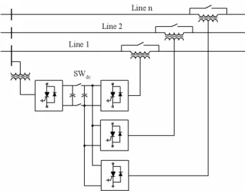
Recently, some new devices have been put forward within the FACTS technology, namely: the IPFC (Interline Power Flow Controller) and the GIPFC (Generalized Interline Power Flow Controller). By utilizing these devices, an indepen-dent controllability over each transmission line of a multi-line system, can be achieved. With the cost of the high power semiconductors and converters declining steadily, both the GIPFC and the IPFC (Figure 1) appear as a stand out solu-tion for the power flow control of multi-line systems, instead of using individually controlled UPFCs (Unified Power Flow Controller) in each line.
Despite the existence of some references on this subject (Gyugyi et alii, 1998; Hingorani and Gyugyi, 1999; Far-daneshet alii, 2000; Jianhonget alii, 2002; Diez-Valencia et alii, 2002 and Strzeleckiet alii, 2002) the control ability that these devices present comes also accompanied with a certain degree of complexity in its structure, control system and the possible indirect effects that they may cause upon the network.
(Voltage-Figure 1: Generic representation of a GIPFC (SWdc=ON) and an IPFC & STATCOM (SWdc=OFF)
Sourced Inverter) within the GIPFC is in charge of fulfill-ing the real power demand established by the series invert-ers through the DC link, as well as to support the voltage of the bus where it is connected (Song and Johns, 1999; Sen and Stacey, 1998; Bianet alii, 1996). The series voltage in-jected to each line can be controlled in both its magnitude (0≤ Vc_i ≤ Vcmax_i )and phase angle (0≤θc_i ≤360˚). The subscriptiin these voltage and angle ranges refers to any of the series converters present in the whole system.
The GIPFC & IPFC steady-state operation also requires that the sum of the active power, exchanged by the total num-ber of converters, be zero. Under certain conditions such as when no voltage support in the substation bus is required, the shunt converter can be dispensed with and the GIPFC (now an IPFC) will be basically constituted by SSSCs (Static Synchronous Series Compensators) connected one to another through a common DC capacitor. In this case, the real power required for varying the angular position of the series volt-ages, will have to be supplied from one of the compensated AC systems. Under both configurations (GIPFC & IPFC), the primary inverter(s) or assisted system(s), will have prior-ity over the secondary inverter (within the assisting system) in achieving its set-point requirements.
2
GIPFC & IPFC MODELING AND
ANALY-SIS
The steady-state analysis developed in this section consid-ers a GIPFC linking two balanced independent AC systems (Figure 2). For ease of analysis, the equivalent sending and receiving-end sources in both systems were regarded as stiff AC sources (infinite buses). It was also assumed that
Sys-Figure 2: Elementary GIPFC system used in the analysis
tems 1 and 2 (or primary and secondary systems, respec-tively) have identical line parameters, although in practice they would usually be different. For heavy and simultaneous compensation in both systems, the shunt converter will have to be properly rated so as to attend the requirements of all the series inverters in operation. Another assumption regarded in this section is that each converter behaves as a shunt or series source operating with fundamental frequency and character-ized by ideal sinusoidal waveforms (Uzunovicet alii, 1998; Vasquez-Arnez and Zanetta, 2005a).
The developed model makes use of the instantaneous power theory (Akagiet alii, 1984) and theds−qsorthogonal co-ordinates (Keriet alii, 1999). Both tools proved to be suitable for the steady-state analysis, as they facilitated the control of the direct and quadrature magnitudes of the ideal sources representing the inverters.
The power equality between the shunt and the series invert-ers, so as not to absorb nor to generate active power from or to the AC system, was strictly applied to the model. Thus, it can initially be established that:
Psh= m X
i=1
Pse_i (1)
In (1), m stands for the total number of series converters. In our case m=2, therefore, using the ds −qs orthogonal components ofIshandV22for the real powerPsh(derived from busV22), it can be written:
Psh=V22dIshd+V22qIshq (2)
Pse1 =Vc1dI14d+Vc1qI14q (3)
Pse2 =Vc2dI24d+Vc2qI24q (4)
Likewise, the reactive power injected (or absorbed, depend-ing on the mode of operation) by the shunt converter can be expressed as:
Qsh=V22dIshq−V22qIshd (5)
So, from Figure 2 the following relations for Systems 1 and 2 can be written:
V22(d,q)+Vc2(d,q)=Z24I24(d,q)+V24(d,q) (6)
V12(d,q)+Vc1(d,q)=Z14I14(d,q)+V14(d,q) (7)
Regarding the shunt current,Ish, as being derived from bus
V22:
I21(d,q)=Ish(d,q)+I24(d,q) (8)
also,
V21(d,q)−V24(d,q)+Vc2(d,q)=Z21I21(d,q)+Z24I24(d,q) (9)
similarly for System 1,
V11(d,q)−V14(d,q)+Vc1(d,q)= (Z11+Z14)I14(d,q) (10)
Equations (6) through (10) are represented in a simple way only to shorten the set of equations. In order to relate them to eqs. (1) and (5), they should also be written in theirds−qs components, which in this case coincide with the real and imaginary axis. By manipulating equations (1) through (10), it will be obtained a set of 10 equations (some of them non-linear) that can be solved using any iterative method. Once computed the unknown variables (i.e. theds−qscomponents ofV12,V22,Ish,I14,I24), the power flow in the
receiving-end of Systems 1 and 2, with or without the series and shunt compensation effect, can be easily calculated through (11). The horizontal line above each variable in (11) and (12) de-notes that such variables are phasors.
S1= (P1+jQ1) = ¯V14I¯14∗; (11)
S2= (P2+jQ2) = ¯V24I¯24∗
In this model, the inclusion of the series transformers’ cou-pling reactance Xse(1,2) within impedances Z14 and Z24,
was only done to shorten the system equations. Once com-puted the line current (I14), the voltage V13 can be
calcu-lated through (12). The bus voltageV23(System 2) can be
obtained through a similar procedure.
¯
V13= ¯V12+ ¯Vc1−jXse1I¯14 (12)
The GIPFC mathematical model developed in this section is also valid for the case of a classical IPFC configuration. Since the shunt VSI is no longer present in the secondary (assisting) system, some of the variables in the above equa-tions will have to be zeroed (i.e.Ishd=0,Ishq=0 andQsh=0). Under this configuration, System 1 (master) will have two independently controlled variables (i.e. Vc1, θc1).
Con-versely, System 2 (slave) will have to provide the series real power demanded by System 1, thus, leaving only one vari-able (Vc2q)to be independently controlled. The above de-scription implies that for the case of a classical IPFC scheme, the real power exchange of converter 2 is pre-defined (i.e. there exists a constraint for System 2) and therefore, only its series reactive compensation can utterly be utilized to control the power flow in this line (similar to the action of an SSSC).
3
SIMULATION RESULTS
In order to assess the effect and control ability of the GIPFC and the IPFC, it will be examined the behavior of the active power flow (which will follow the behavior of its respective line current) at the receiving-end of both systems.
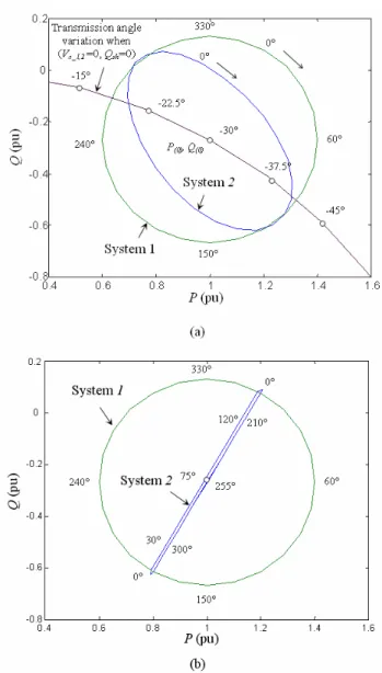
TheP −Qplane results shown in Figure 3 were obtained using the mathematical model developed in Section 2. Each series angle (θc1, θc2)corresponding to Vc1 and Vc2 were
simultaneously varied from 0 to 360 degrees. The regions inside the ideal circle and inside the ellipse, correspond to the controlled area provided byVc1 and Vc2, respectively.
Among the reasons responsible for the obtention of the pat-tern showed in Figure 3(a), are: firstly, the real power de-mand of the series converter in System 1 (which must be ful-filled by the shunt converter) imposes a voltage variation to busV22, mainly to those series angles comprised in the range
θc1 ≈330˚→60˚ and 150˚→240˚, in whichPse1demands
a substantial amount of the exchanged real power. Secondly, the location of the shunt converter (i.e. modification ofZ21)
in relation to the sending-end bus (V21)was also observed to
Figure 3:P−Qplane at the receiving-end of Systems 1 and 2: (a) GIPFC withVc1=0.2 pu &Vc2=0.15 pu (b) IPFC case
(Vc1=0.2 pu) &Vc2=f(Vc1)
Should the shunt VSI be connected to an independent line, both Systems 1 and 2 will ideally present a circular con-trol region as none of them will affect the other’s voltage or power characteristics. A similar result will be obtained whenZ11 = Z21 ∼=0, as in this case, voltagesV11 &V21
(stiff sources) will take over from voltagesV12 &V22,
re-spectively.
Also in this case (Figure 3a), no shunt reactive power (Qsh=0) was applied to busV22. During the uncompensated
condition (i.e. when Vc1 = Vc2=0) the real and reactive
power in each system (receiving-end) were equal toP1(0) =
P2(0) = 1.0pu andQ1(0) =Q2(0) = −0.2679pu,
respec-tively. For all the simulated cases, the sending and receiving-end sources in both systems were set to V11 =V21=1.06 0˚
andV14=V24=1.06 -30˚ pu.
Figure 3(b), shows the power flow behavior of a two-inverter IPFC in whichVc2, due to the IPFC inherent operation,
be-comes a function of voltageVc1(specified). The straight line
observed in this result represents the power flow variation experienced by System 2 on account of the help provided to System 1 for manipulating its power flow.
The latter statement does not imply that inverter VSI-2 (Sys-tem 2) will be unable to compensate simultaneously to its own line. It can execute local compensation with its available series reactive power. Under these conditions the straight line observed in Figure 3(b) will be shifted to the left (in-ductive mode) or to the right (capacitive mode of compen-sation), thus, establishing a square-like skewed area whose control region will again be limited by the capacity of the in-verter. Recall that, quadrature voltage injection with respect to the line current, has predominant effect upon the line’s real power flow. In-phase voltage injection has predominant ef-fect on the line’s reactive power flow and it is associated to the real power exchange between the converters (Vasquez-Arnez and Zanetta, 2005b).
Notice that, asVc1approaches to the quadrature position with
respect to the line current (in our caseθc1=75˚, 255˚) bothP2
andQ2on System 2 (Figure 3b), return to the uncompensated
condition (i.e. P2(0)&Q2(0)). This is due to the less
(even-tually null) demand in the exchanged power (Pse1)between
the series-connected VSIs (i.e. voltageVc1 is in quadrature
with respect toI14).
So, it can be stated that while the power flow in System 1 (P1) can be set to operate in an uncompensated mode
at P1(0)=1.0 pu, with solely System 2 being compensated
throughVc2, the opposite operative condition (i.e. System 1
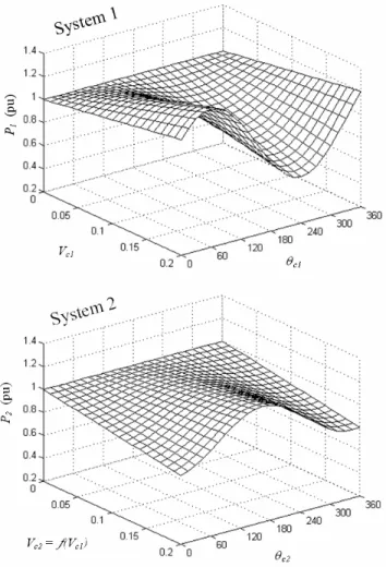
being compensated and System 2 kept unaltered) will present a drawback. That is, it is not possible to maintain unaltered the power flow over System 2 atP2(0)=1.0 pu, when solely
System 1 is being compensated. This fact can be better ob-served in Figure 4. As the module of the series voltage in System 1 is increased (Vc1=0 →0.2 pu) controlling
effec-tively the real power (P1), the active power flow in System
2 (P2)becomes proportionally affected. Recall thatVc2and
Pse2are related through (4), in turnPse2andPse1are related
through (1).
This voltage and power flow degradation that System 2 expe-riences was observed to occur in both FACTS devices. Yet, in the GIPFC configuration, the voltage variation that busV22
experiences, while helping to manipulate the series voltage
Vc1, can be largely controlled through the shunt converter’s
Figure 4: Power flow control in System 1 and its effect upon System 2 (uncompensated) whenVc1= 00.2pu (IPFC
con-figuration)
As for the IPFC configuration, it was also observed that in-dependently of the inverters’ position along the line, the ef-fect of converter VSI-1 upon VSI-2 (unless the real power exchanged between them be zero), will occur.
The algorithm built in MatlabR, related to the model pre-sented in Section 2, enabled to explore and test some other operative conditions. For example, it was observed the con-dition whenVc1<Vc2(e.g. Vc1=0.10 pu or less andVc2kept
constant atVc2=0.15 pu). Under this condition, System 1 (as
expected) maintained its circular pattern within the ellipse. As for System 2, the conditionVc1<Vc2(whenVc1=0.15→
0.0 pu) drew a lesser ellipticalP2−Q2region proportional
to the value ofVc1. DespiteVc1=0, the operative region in
System 2 did not draw a perfectly circular area, as inverters VSI-2 and VSIsh(Figure 5) will still be operating as a UPFC (Keriet alii, 1999 ), unless the series converter be modeled as an ideal source able to supply (or absorb) independently
Figure 5: GIPFC scheme linking Systems 1 and 2
active and reactive power to (or from) the line.
3.1
GIPFC & IPFC Overall Control System
The ATP program built to simulate the GIPFC scheme shown in Figure 5 is based upon the work published by Vasquez-Arnez and Zanetta (2005a), where it was presented a UPFC using similar control techniques and features. The wave-forms generated with the GIPFC scheme were obtained us-ing a 12-pulse 3-level converter configuration that utilized the phase-shift control technique, with GTOs (Gate Turn-Off thyristors) as switching devices. In this ATP program, both equivalent AC systems were assumed to operate at a rated voltage of 230 kV. The shunt converter’s rated power was set to±200 MVA, a fair amount to fulfil the maximum real power demand from both series VSIs (each with a rated power of 100 MVA) and to compensate, through its avail-able shunt reactive power, the bus voltageV22. The coupling
transformers were chosen regarding firstly, the rated power of each converter and secondly, the DC link rated voltage which in our case was equal to 25 kV.
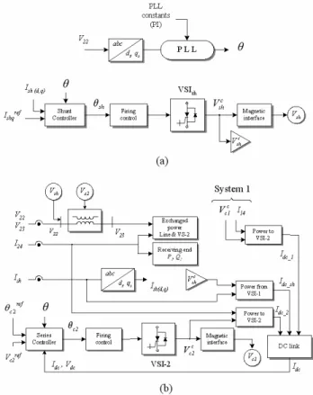
The GIPFC control system illustrated in Figure 6, used to built the ATP program, is based upon PI (Proportional-Integral) controllers. For the sake of space limitations, it will be assumed that the sequence of the whole control block dia-gram presented can effortlessly be followed. Therefore, only the internal operation of the shunt and series controllers (con-trol boxes) depicted in Figures 6(a) and (b), will be described.
Within the shunt controller illustrated in Figure 6(a) an error between the quadrature component of the measured (Ishq) and the specified (Ishqref)shunt current, is initially established. This error is translated into an angle, which when added to
Figure 6: Control block diagrams of the: (a) shunt converter, (b) series converter
system is used to control the dc link voltage. The voltage
Vc
sh generated by VSIsh will present a raw waveform, so before inserting it to busV22 it should be properly shifted
(thus improved) by the magnetic interface (Vasquez-Arnez and Zanetta, 2002).
As for the series controller operation illustrated in Figure 6(b) the addition ofθ andθrefc2 result in a preliminary
an-gle. This angle, along with the so called dead angle (period between the positive and negative waveform and which de-termines the operation of an inverter either as a 3-level or 2-level inverter) obtained from the relation betweenVcref2 and
Vdc, will constitute the phase angle used in the firing control of the series converter (Sen and Stacey, 1998). The control block diagram of the series converter in System 1, will be simpler than the control system presented for System 2. Re-call that in the former, the shunt converter is dispensed with from the arrangement. Note also that in the ATP program used, unlike the program written in MatlabR, it was speci-fiedIshq instead ofQsh.
Care must be taken during the implementation of the DC cir-cuit which establishes the dependence between the shunt and the series inverters, as there must exist a continuous exchange between both converters. Neither unbalanced nor systems
Figure 7: Control block diagram used in the IPFC configura-tion
having a high harmonic content can be accurately studied us-ing the developed models, as they are based upon balanced system conditions and sinusoidal (or quasi sinusoidal) volt-age and current waveforms. These aspects and conditions are left for further research.
The control system of the two-inverter IPFC illustrated in Figure 7, presents some differences in relation to the GIPFC case. Each VSI in the IPFC scheme is usually synchronized to its own line current through independent PLLs. By doing so, each VSI can independently supply series reactive com-pensation to its own line. That will also make possible the operation of any of the VSIs during contingency conditions when either converter (or system) is out of service.
Briefly, each angleθ1andθ2(calculated by its own PLL) are
used to transform the input variables to theirds−qs (orthog-onal) components. The error betweenVcref1(d,q)andVc1(d,q)
(primary system) is amplified to calculate the module and angle of the preliminary series voltage. The final series angle used in the VSI-1 firing logic, is obtained from the addition ofθ1+θc1. The real powerPse1demanded by this inverter
(VSI-1), which appears as a demand to be fulfilled by in-verter VSI-2, is calculated using the instantaneouspqpower theory.
The negative sign of Pse2 stems from the constraint
(Pse1+Pse2) = 0. As the value ofPse1 is imposed by
the primary (master) system, then the Vc2d component can be obtained through (4). Recall that in the secondary (slave) system the Vc2q component can be specified. Similarly to the case of System 1, the final series angle to be used by the converter’s firing logic is obtained from (θ2+θc2).
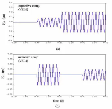
Figure 8: GIPFC power flow control over Systems 1 & 2,
Vc1 = 0.106 60˚ at t1= 0.1s,Vc1= 0.206 60˚ at t2= 0.2s,
Vc2 = 0.106 240˚ at t1 = 0.1s,Vc2 = 0at t2 = 0.2sand
Vc2= 0.056 240˚ at t3= 0.3s.
flow control sequence over both systems can be summed up as follows: due to system requirements at t=0.1 sP2 is
re-duced, whereasP1 (System 1) is increased. Subsequently,
the power flow reduction effect ofP2is cancelled out (t=0.2
s) whereasP1, on account of an hypothetical greater demand,
is increased even more. The final control action occurs at t=0.3 s whenP2 is, due to a system requirement too, once
again forced to reduce its transmitted power.
The amplitude variation of the series voltages injected (Vc1,
Vc2) characterizing the effect of the power flow behavior
shown in Figure 8, can be observed in Figure 9.
On the other hand, Figure 10 shows the referred slight power flow degradation (∆P2)experienced by System 2 and which
was mentioned in Section 3. The small oscillations observed at the beginning of each control action (points A & B in Fig-ure 10) are due to the PI (Proportional-Integral) controller adjustment and can be set and improved manually.
The GIPFC implemented in ATP provided to each line a high degree of controllability, as the transmitted power was simul-taneously (and almost instansimul-taneously) reduced or increased according to the operative needs of either system.
It should be noted that the multi-line FACTS controllers an-alyzed herein are primarily aimed to the power flow con-trol. Nowadays, the FACTS technology offers various types of devices to cope with the various needs and applications within a power system, most of them still in the research stage, though. Problems existing within two independent asynchronous systems (or systems having different frequen-cies), for example, may well be tackled by using two shunt-connected VSIs whose DC sides are mutually shunt-connected (similarly to a back-to-back HVDC configuration). Still, some other problems such as system dynamic disturbances can be dealt with using series-connected VSIs, such as the
Figure 9: Series voltages(Vc1, Vc2injected to Systems 1 and
2
IPFC (Noroozianet alii, 1997).
4
OPERATIONAL CONSTRAINTS
Despite the benefits brought by the FACTS devices studied herein, there are also a number of operative constraints and limitations that should be accounted, like those described and explored in this section.
Figure 10: Power flow control over System 1,Vc1=0.106 60˚
4.1
Line Voltage Limitations
During steady-state, certain system restrictions can give place to limitations in the operative areas of both FACTS devices (GIPFC and IPFC). Such sub-areas, which will be referred to as NOAs (Non-Operative Areas), are due to the boundaries of voltagesV12,V13,V22 andV23shown in
Fig-ure 2 (which should not be violated).
Briefly, the module of each series voltage in the model pre-sented in Section 2, was set toVc1=Vc2= 0.2 pu and rotated
along the 360˚. While doing so, there appeared values of
V12,V13,V22andV23 which were out of the operative
volt-age range imposed, thus, producing the NOA areas.
Figure 11, shows the NOA areas stemming from these volt-age boundaries established (±10% of the nominal voltvolt-age in the referred buses, i.e. 0.9 ≤Vi2&Vi3 ≤1.1pu) which
will in turn modify the ideally circular operative region of the series voltages injected. Although in our case voltagesV12
&V22are internal voltages, in classical schemes they might
represent the substation voltage. The smaller NOAs obtained for System 2 (Figure 11b), are because the bus voltage (V22)
was compensated by the reactive power (Qsh)from the shunt VSI (capacitive mode), thus, improving its voltage limits.
As the series voltage magnitude (Vc1orVc2)is increased, and
if no other parameter in the system is altered, there will exist a trend among the NOA parabolic curves to cross each other, thus, increasing the NOA areas.
On the other hand, if voltagesV13 andV23 would be more
flexible in their voltage operation range, it could contribute to the reduction of the NOAs. Of course, this should be in ac-cordance with the specifications of the line’s maximum volt-age withstanding capacity.
4.2
Shunt Converter Rating Constraint
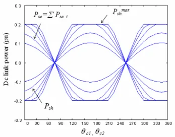
An effect similar to that shown in Figure 11 (creation of non operative areas) will also occur in cases when the assisting converter’s capacity (VSIshin the GIPFC case or the sec-ondary system inverter in the IPFC configuration) can not fulfill the demand of the series VSIs. In that case, the shaded areas (NOAs) will slide further downwards in relation to the positions shown in Figure 11. The shunt converter’s capacity is commonly determined by:
M V Ashunt= v u u t
m X
i=1
Pse_i !2
+ (Qshunt)2 (13)
In a work published by Songet alii(2000), it is suggested that whenever a limit is going to be violated by a variable,
it would be preferably to set the violated variable (in the re-maining computation process) at its limiting value in order to achieve the highest efficiency of the compensator.
So, in line with the above statement and because the shunt VSI has a limited capacity, it was established that whenever
Figure 11: GIPFC Non-Operative Areas (NOA) correspond-ing to: (a) System 1, (b) System 2 withQsh=0.1 pu.
the maximum rated real power was going to be surpassed, the exceeding value would be limited to its maximum value (e.g.Pmax
sh =±0.2 pu as seen in Figure 12).
Figure 12, also shows the power balance between the shunt and the series inverters. Notice that any Pse curve (total power demanded by the series VSIs) along the full range of the series angles (θc1,θc2)has an identical, but opposite,
be-havior (if losses within the inverters are neglected) than the real power supplied by the shunt converter (Psh). ThePshmax limitation will impose a detrimental effect upon the series in-verters’ active power and thus onVc1andVc2, creating non
operative regions like those presented in Section 4.1. For the IPFC configuration, the real power limitation due to the sec-ondary system’s inverter rating, showed a similar result.
4.3
Maximum Power Exchange through
the DC-Link
The maximum real power transferred through the dc-link by the inverter in the secondary system, can impose another re-striction to the operation of the GIPFC and IPFC. Therefore, it is important to identify which will be the steady-state max-imum power that can be exchanged through the dc-link to fulfill the demand of the series inverter(s). The power enter-ing each series inverter (see the dc-link circuit of Figure 5), can be written as:
Pdc1=VdcIdc1 ; Pdc2=VdcIdc2 (14)
Also, the AC side real power coming out from each inverter, can be expressed as:
Pse1=ℜe V¯c1I¯14∗
; Pse2=ℜe V¯c2I¯24∗
(15)
If the losses within the inverters are neglected, then (14) can be equated to (15). On the other hand, the line current over System 1 can be written as:
¯
I14=
¯
V11+ ¯Vc1−V¯14
jX
(16)
where: X represents the equivalent series reactance of the line.
Manipulating equations (15) and (16), yield,
Pse1=
Vc1
X [V11(sinδ11cosθc1−cosδ11sinθc1) + V14(cosδ14sinθc1−sinδ14cosθc1)] (17)
Similarly for System 2,
Pse2=
Vc2
X [V21(sinδ21cosθc2−cosδ21sinθc2) +
V24(cosδ24sinθc2−sinδ24cosθc2)] (18)
Notice that, due to an earlier assumption, the equivalent line reactance in (18) is similar to that of System 1. As for the IPFC analysis, the shunt VSI should be disconnected from the scheme (Figure 5). The derivative of (17) with respect to
θc1will allow us to calculateθc1, thus to obtain the maximum
power (Pmax
se1 )corresponding to inverter 1.
dPse1
dθc1
= d
dθc1
V c1
X [V11(sinδ11cosθc1−cosδ11sinθc1) +
V14(cosδ14sinθc1−sinδ14cosθc1)]}= 0 (19)
θc1=tan−1
V14cosδ14−V11cosδ11
V11sinδ11−V14sinδ14
(20)
So, regarding the assumption made earlier on (in this section) about the converter losses, it can be considered that this max-imum power will correspond to the power transferred via the DC link to the series inverter in System 1. As for the GIPFC configuration, a similar procedure, regarding the derivative ofPse2 with respect toθc2 and the substitution ofθc2 into
(18), will have to be realized for System 2. Finally, the to-tal maximum power transferred by the shunt VSI will result from the addition of them(in our case two) series inverters’ real power, as stipulated in (1).
5
CONCLUSIONS
Finally, to evaluate the dynamic response and validate the initially developed fundamental frequency analysis, a 12-pulse phase-shift VSI-based GIPFC, was also elaborated in the ATP program. The simulations performed and their re-sults supported the steady-state model initially presented, as well as showed in a more stringent way the GIPFC capabili-ties and its associated drawbacks.
REFERENCES
Akagi, H.; Kanazawa, Y. and Nabae, A. (1984). Instan-taneous Reactive Power Compensators Comprising Switching Devices without Energy Storage Compo-nents, IEEE Trans. on Power Industrial Applications, Vol. 20, No. 3, pp. 625-631.
Bian, J.; Ramey, D.G.; Nelson, R.J. and Edris, A. (1996). A Study of Equipment Sizes and Constraints for a Unified Power Flow Controller (UPFC).Proc. IEEE/PES-1996 Transmission and Distribution Conference, L.A., Cali-fornia, pp. 332-338.
Diez-Valencia, V.; Annakkage, U.D.; Gole, A.M.; Dem-chenko, P. and Jacobson D. (2002). Interline Power Flow Controller (IPFC) Steady State Operation.Proc. Canadian Conference on Electrical and Computer En-gineering, IEEE CCECE 2002, Vol. 1, pp. 280-284.
Fardanesh, B.; Shperling, B.; Uzunovic, E. and Zelingher, S. (2000). Multi-converter FACTS Devices: the General-ized Unified Power Flow Controller (GUPFC). Proc. IEEE Power Engineering Society Summer Meeting, 2000, Vol. 2, pp. 1020 - 1025.
Gyugyi, L.; Sen, K.K. and Schauder, C. D. (1998). Inter-line Power Flow Controller Concept: A New Approach to Power Flow Management in Transmission Systems, IEEE Transactions on Power Delivery, Vol. 14, No. 3, pp. 1115-1123.
Hingorani, N.G. and Gyugyi, L. (1999). Understanding FACTS: Concepts and Technology of Flexible AC Transmission Systems, IEEE Press, N.Y.
Jianhong, C.; Lie, T.T. and Vilathgamuwa D.M. (2002). Basic Control of Interline Power Flow Controller. Proc. IEEE Power Engineering Society, Winter Meet-ing 2002, Vol. 1, pp. 521-525.
Keri, A.J.F.; Mehraban, A.S.; Lombard, X.; Eiriachy, A.; Edris, A.A. (1999). Unified Power Flow Controller (UPFC): Modeling and Analysis,IEEE Transactions on Power Delivery, Vol. 14, No. 2, pp. 648-654.
Noroozian, M.; Angquist, L.; Ghandari, M. and Ander-son, G. (1997). Improving Power System Dynamics by
Series-Connected FACTS devices,IEEE Trans. Power Delivery, Vol. 12, pp. 1635–1641.
Sen, K.K. and Stacey, E.J. (1998). UPFC-Unified Power Flow Controller: Theory, Modeling and Applications, IEEE Transactions on Power Delivery, Vol. 13, No. 4, pp. 1953-1960.
Song, Y.H. and Johns, A.T. (1999).Flexible AC Transmission Systems - FACTS, IEE Press, London.
Song, Y.H.; Liu, J.Y. and Mehta, P.A. (2000). Strategies for Handling UPFC Constraints in Steady-State Power Flow and Voltage Control,IEEE Transactions on Power Systems, Vol. 15, No 2, pp. 566-571.
Strzelecki, R.; Benysek, G.; Fedyczak, Z. and Bojarski, J. (2002). Interline Power Flow Controller-Probabilistic Approach.Proc. IEEE 33rdAnnual Power Electronics Specialists Conference, PESC, Vol. 2, pp. 1037-1042.
Sun, J.; Hopkins, L.; Shperling, B.; Fardanesh, B.; Gra-ham, M.; Parisi, M.; MacDonald, S.; Bhattacharya, S.; Berkowitz, S.; Edris, A. (2004). Operating Char-acteristics of the Convertible Static Compensator on the 345 kV Network.Proc. IEEE-PES Power Systems Conf. and Exp., Vol. 2, pp. 732-738.
Uzunovic, E.; Cañizares, C. and Reeve, J. (1998). Fun-damental Frequency Model of Unified Power Flow Controller.Proc. North American Power Symposium -NAPS 1998, Cleveland, Ohio, pp. 294-299.
Vasquez Arnez, R.L. and Zanetta Jr. L.C. (2002). 48-Pulse Based SSSC (Static Synchronous Series Compensator) an Evaluation of its Performance. Proc. WSEAS In-ternational Conferences on: System Science, Applied Mathematics & Computer Science and Power Engi-neering Systems, Rio de Janeiro.
Vasquez-Arnez, R.L. and Zanetta Jr, L.C. (2005a). Compen-sation Strategy of Autotransformers and Parallel Lines Performance, Assisted by the UPFC, IEEE Transac-tions on Power Delivery, Vol. 20, No. 2, pp. 1550-1557.
Vasquez-Arnez, R.L. and Zanetta Jr, L.C. (2005b). Multi-Line Power Flow Control: An Evaluation of the GIPFC (Generalized Interline Power Flow Controller). Proc. 6th International Conf. on Power Systems Transients – IPST’05, Montreal,