Discretization and event triggered digital output feedback control of LPV systems

Contents lists available atScienceDirect

Systems & Control Letters

journal homepage:www.elsevier.com/locate/sysconle

Discretization and event triggered digital output feedback control of

LPV systems

Márcio F. Braga

a

, Cecília F. Morais

a

, Eduardo S. Tognetti

b

, Ricardo C.L.F. Oliveira

a

,

Pedro L.D. Peres

a,∗

a_{School of Electrical and Computer Engineering, University of Campinas — UNICAMP, 13083-852, Campinas, SP, Brazil}

b_{Department of Electrical Engineering, University of Brasilia — UnB, 70910-900, Brasília, DF, Brazil}

a r t i c l e i n f o

Article history:

Received 1 December 2014 Received in revised form 11 August 2015 Accepted 12 October 2015 Available online 11 November 2015

Keywords:

Discretized linear systems Networked control systems Taylor series expansion Output feedback control Time varying parameters Linear matrix inequalities

a b s t r a c t

This paper investigates the problem of discretization and digital output feedback control design for continuous-time linear parameter-varying (LPV) systems subject to a time-varying networked-induced delay. The proposed discretization procedure converts a continuous-time LPV system into an equivalent discrete-time LPV system based on an extension of the Taylor series expansion and using an event-based sampling. The scheduling parameters are continuously measured and modeled as piecewise constant. A new transmission of the measured output to the controller is triggered by significant changes in the parameters, yielding time-varying transmission intervals. The obtained discretized model has matrices with polynomial dependence on the time-varying parameters and an additive norm-bounded term representing the discretization residual error. A two step strategy based on linear matrix inequality conditions is then proposed to synthesize a digital static scheduled output feedback control law that stabilizes both the discretized and the LPV model. The conditions can also be used to provide robust (i.e., independent of the scheduling parameter) static output feedback controllers. The viability of the proposed design method is illustrated through numerical examples.

©2015 Elsevier B.V. All rights reserved.

1. Introduction

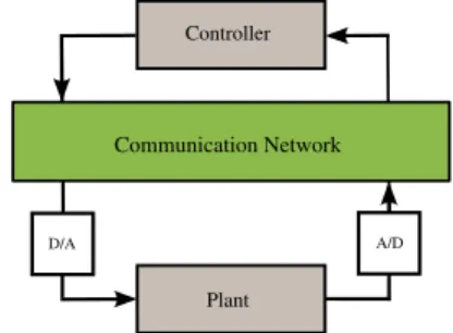
Due to technological advances, in many practical applications, the use of communication channels to implement control projects has considerably increased [1]. For instance, the exchange of data between control system components can be done by employing a networked control system (NCS) architecture. Some advantages of this framework are the use of plug-and-play devices, ease of system maintenance and diagnosis, increased system agility, and reduction in system wiring. However, despite of those benefits, some well known NCS drawbacks, like packet dropouts, multiple-packet transmission, bandwidth requirements, and network-induced delay [2,1] can restrict its use. Such disadvantages have received considerable attention from the control community, which is continuously looking for solutions to overcome the difficulties arising from the use of an NCS architecture [3–7].

In an NCS framework, the control strategy usually comprises a continuous-time plant controlled by a discrete-time controller

∗_{Corresponding author.}

E-mail address:peres@dt.fee.unicamp.br(P.L.D. Peres).

interfaced by analog-to-digital (A/D) and digital-to-analog (D/A) devices. This structure gives rise to two important matters that must be jointly dealt with: first, the continuous-time system can be affected by uncertainties, which occur owing to parameter variations, external perturbations, noises, the inaccuracy of sensors and actuators or related to hidden dynamics [8]; and, second, the necessity to design a digital controller that assures the stability of the closed-loop hybrid system (continuous-time plant and digital controller).

For the first problem, a possible solution is the employment of the linear parameter-varying (LPV) system theory, see [9,10] and references therein. LPV modeling has increasingly evolved in the last years, mainly to represent non-linear systems in terms of a family of linear models and to describe systems whose dynamic is affected by parameters that can vary arbitrarily fast or have known bounds on the their rate of variation [11]. The second issue, generally, requires a procedure to discretize the continuous-time equations which represent the plant model (see [12] for a more detailed discussion on different ways to design digital controllers). An important observation regarding this issue is that most of the discretization approaches can only deal with plants free of uncertainties (i.e., precisely known systems) [13], or use

approximated numerical methods that neglect the discretization error [14].

An interesting digital control approach that deals with impul-sive systems and hybrid methods considering the inter-sampling behavior is presented in [15]. Following similar lines, a simpli-fied assumption of control design for continuous-time LPV systems is employed in [16] for a class of piecewise constant parameters under constant and minimum dwell-time. Nevertheless, in the lit-erature, there are only a few works that cope with the discretiza-tion of LPV systems. For instance, in [17,18], the authors provide conditions to design, respectively, state and output feedback dig-ital controllers for LPV systems with desired performance speci-fications by employing the lifting technique [19]. Other examples can be found in [20,21], where a digital controller or filter is de-signed through the same approach, assuming the time-varying pa-rameters are piecewise constant. Those papers assume that both the discretization procedure and the design of the controller or fil-ter are performed in real time, that is, the time-varying parame-ters are continuously read and, at each sample, a new discrete-time model related to the continuous-time plant for the current param-eter is computed, and the synthesis conditions are re-evaluated. In this framework, the plant is an LTI system and the discrete-time model is exact, because, for each fixed parameter, the continuous-time system becomes precisely known. Nevertheless, this tech-nique presents, as drawback, a large processing burden for its implementation, since the discrete-time model is computed and the design conditions are solved in real time.

This paper proposes a discretization procedure, based on an extension of the Taylor series expansion of an arbitrary degree

ℓ, which converts a continuous-time LPV model with piecewise

constant parameters and a time-varying network-induced de-lay into an equivalent discrete-time LPV system. The accuracy of the discrete-time representation is strongly related to the in-crease of degree

ℓ. An event-based sampling of the output

asso-ciated to the changes of the time-varying parameters is assumed. Thus, as discussed in [18], by considering the hypothesis of a time-varying sampling interval that depends on the system parameter measurements, it is possible to treat a broad class of problems, such as engines, manufacturing systems and telerobotic systems. For instance, one can cite an internal combustion engine whose sampling interval is variable and depends on the engine speed [18]. Differently from the discretization procedure proposed in [22] for uncertain time-invariant systems, the new method pre-sented in this paper considers that the network-induced delay in the continuous-time LPV system can be time-varying. The ob-tained discretized model, with bounds on the rate of variation of the parameters, is described by homogeneous polynomial matri-ces of degree

ℓ

on the time-varying parameters, which belong to the Cartesian product of simplexes (called a multi-simplex [23]), plus a norm-bounded term related to the approximation error. The norm-bounded term depends on the degree of Taylor series expan-sion, the sampling time, the network-induced delay, and the origi-nal continuous-time uncertainty domain. Estimates for the bounds of the discretization residual error terms are computed through a grid in the uncertainty domain. To establish a valid discrete-time LPV representation, the discrete-time-varying parameters considered in the continuous-time model are supposed piecewise constant and, therefore, the parameters do not change between two consec-utive samples. Considering that the parameters are continuously monitored and have known bounds on their rate of variation, a new transmission is triggered to sample the output and the sched-uled parameters whenever a significant change occurs. Otherwise, a new sample is acquired when a prescribed upper bound on the transmission interval is reached. In this scheme, the assump-tion that, during the sampling interval, the parameter variaassump-tions are insignificant and can be neglected is valid, as considered in

Fig. 1. Illustration of the networked control system investigated. [16–18,20,21]. The value of the upper bound on the rate of vari-ation of the parameters is used to specify a lower bound for the sampling period and to prevent the so-called Zeno behavior [24].

Therefore, the proposed methodology can be viewed as a parameter-based event sampling technique that can be used to deal with a wide variety of LPV systems. Compared to the usual strategy that imposes a constant small sample period to cope with abrupt variations, requiring a large bandwidth and increasing the network traffic load, the approach proposed in this paper repre-sents an important contribution in the context of NCS.

Additionally, new conditions for state and output feedback con-trol design of discrete-time polynomial systems with time-varying parameters are proposed in terms of linear matrix inequalities (LMIs). The conditions are solved by LMI relaxations that take into account the bounds on the rates of parameter variations. An ex-tension of the two stage strategy [25–28] is used to provide a stabilizing static output feedback control law: initially, a parameter-dependent state feedback gain is synthesized; then the outcome is applied in the second step, where a parameter-dependent output feedback controller is determined. To implement the scheduled output feedback control law, it is assumed that the time-varying parameters of the continuous-time plant can be measured or esti-mated in real time. If this is not the case, the conditions can also be used to determine a robust control law (parameter-independent). The use of polynomial parameter-dependent Lyapunov matrices and slack variables of arbitrary degrees in the proposed LMI relax-ations can reduce the conservativeness of the synthesis conditions. The applicability of the proposed method is illustrated through nu-merical examples.

The remainder of the paper is structured as follows. Section2

presents the notation, the proposed discretization technique and the event-triggered control modeling employed in this paper. Sec-tion3introduces the main results for the state and output feedback control design procedure. Section4provides numerical examples and, finally, Section5summarizes the paper.

2. Problem statement

Consider a continuous-time time-varying linear system trolled through a network communication channel by a digital con-troller, as illustrated inFig. 1.

For control purposes, the following continuous-time LPV model with piecewise constant parameters is used



_˙

_x

₍

_t

₎

₌

_E

_(α

1

(

t

))

x

(

t

)

+

F

(α

1

(

t

))

u

(

t

−

τ (

t

))

y

(

t

)

=

G

(α

1

(

t

))

x

(

t

)

t

≥

0, x

(0)

=

0, u

(

V

₎

=

0, V

∈ {−

τ (

t

),

0

}

,

(1)

Rnx×nx_,F

_(α

₁

₍

_t

₎₎

_∈

Rnx×nu_{, andG}

_(α

₁

₍

_t

₎₎

_∈

Rny×nx_are parameter-dependent and can be written as a convex combination of N1 known vertices

(

E

,

F

,

G

)(α

1

(

t

))

=

N1



i=1

α

1i

(

t

)(

Ei

,

Fi,Gi

)

(2)

where

α

1

(

t

)

=

(α

11

(

t

), . . . , α

1N1

(

t

))

is assumed to be a piecewise

constant parameter vector belonging to the unit simplex, given by

ΛNm=



(ζ1, . . . , ζNm)∈R Nm_:

Nm



i=1

ζi=1, ζi≥0,i=1, . . . ,Nm



.(3)

The main objective of this paper is to synthesize an output feedback digital controller that stabilizes system(1). In order to implement the digital control law, it is necessary to define a technique to sample the output signaly

(

t

)

and the time varying-parameters

α

1

(

t

).

The next subsection details the sampling scheme employed in this paper.

2.1. Event-based sampling technique

Consider a parameter vector

ρ(

t

)

of a typical LPV system that varies continuously and is measured in real-time. The absolute value of the time derivative of

ρ(

t

)

is upper bounded by

σ >

0, that is,

∥ ˙

ρ(

t

)

∥ ≤

σ. Whenever a significant change of

ρ(

t

)

occurs, that is,

∥

1

ρ(

t

)

∥ ≥

ϵ, where

1

ρ(

t

)

=

ρ(

t

)

−

ρ(

tk),tis the current instant,tk

<

t is the last sampling instant of

ρ(

t

), and

ϵ >

0 is chosen by the designer, a new sample ofy

(

t

)

and

ρ(

t

)

is sent through the network. The parameter vector

α

1

(

t

), considered in

the continuous-time model(1), is defined as

α

1

(

t

)

=

ρ(

tk),

∀

t

∈

[

tk,tk+1

). Thus, by choosing a convenient value for

ϵ, the parameter

variations during the sampling interval are insignificant and can be neglected [17,18,20,21]. Since

∥ ˙

ρ(

t

)

∥ ≤

σ

, the minimum value of the elapsed time between two consecutive samples,T

(α

2

(

t

)), is

given by1

Tmin

=

ϵ

σ

,

(4)

because

d

ρ(

t

)

dt

≃

1

α

1

(

kT

(α

2

(

t

)))

T

(α

2

(

t

))

≤

ϵ

Tmin

=

σ

where

1

α

1

(

kT

(α

2

(

t

)))

= ∥

α

1



(

k

+

1)T

(α

2

(

t

))



−

α

1



kT

(α

2

(

t

))



∥ ≤

ϵ.

(5) If no significant changes of

ρ(

t

)

occurs, a new sample is triggered after time Tmax is elapsed from the previous sample. The threshold Tmax, chosen by the designer, is related with the maximum allowable transmission interval [29]. Thus, T

(α

2

(

t

))

varies inside the interval [Tmin

,

Tmax] and

α

2

(

t

)

is a piecewise constant parameter belonging to the unit simplexΛN2,N2

=

2.

In this paper,T

(α

2

(

t

))

is supposed to be greater than

τ (

t

)

and, as the network-induced delay lies inside the interval

[

τ

1

, τ

2

]

, it can be rewritten as

τ (α

3

(

t

))

=



2i=1

α

3i

(

t

)τi, where

α

3

(

t

)

is a piecewise constant parameter belonging to the unit simplexΛN3,

N3

=

2. ThusT

(α

2

(

t

))

≥

τ (α

3

(

t

)),

∀

α

2

(

t

),

∀

α

3

(

t

).

Based on these assumptions, a discretization procedure is proposed in the following subsection.

1 Note that, due to the sampling scheme adopted in this paper, the effect of chattering can be avoided, sinceTmindepends on a parameterϵchosen by the designer. Additionally, the Zeno Behavior phenomenon [24], i.e., the sampling period tending to zero, does not occur.

2.2. Discretization procedure

This paper proposes an equivalent discrete-time LPV model for system(1), as accurate as possible, represented by2



x

(

k

+

1)

=

A

(α(

k

))

x

(

k

)

+

B

(α(

k

))

u

(

k

)

+

Bd(α(k

))

u

(

k

−

1)

y

(

k

)

=

C

(α(

k

))

x

(

k

).

(6) Since the time-varying parameters are considered piecewise constant they do not vary between two consecutive sampling instants, that is,

α(

t

)

=

α(

k

),

∀

t

∈ [

tk, tk+1

), matrices

A

(α(

k

)),

B

(α(

k

))

andBd(α(k

))

can be written as

A

(α(

k

))

=

eE(α1(t))T(α2(t))

B

(α(

k

))

=



Υ(α2,α3)

0

eE(α1(t))s_ds



F

(α

1

(

t

))

Bd(α(k

))

=

eE(α1(t))Υ(α2,α3)



τ (α3(t))

0

eE(α1(t))s_ds



F

(α

1

(

t

)),

(7)

whereΥ

(α

2

, α

3

)

=

T

(α

2

(

t

))

−

τ (α

3

(

t

)).

The time-varying parameters affecting the system, the sam-pling interval and the delay can be gathered in a vector

α(

k

)

=

(α

1

(

k

), α

2

(

k

), α

3

(

k

))

that belongs to the multi-simplex domain ΛN, given by the Cartesian product of the unit simplexesΛNm

,

m

=

1,2,3, as defined below.

Definition 1(Multi-Simplex [23]). A multi-simplex ΛN is the Cartesian productΛN1

×· · ·×

ΛNrof a finite numberrof simplexes

ΛN1

, . . . ,

ΛNr. The dimension of theΛNis defined as the indexN

=

(

N1

, . . . ,

Nr

). For ease of notation,

RNdenotes the spaceRN1+···+Nr. A given element

α

∈

ΛN is a vector belonging toRN and can be decomposed as

(α

1

, α

2

, . . . , αr

)

according to the structure ofΛN and, subsequently, each

αm

(being inΛNm

⊂

R

Nm_),m

₌

_{1, . . . ,r,} is decomposed in the form



αm

1

, αm

2

, . . . , αmN

m



.

To circumvent the difficulty of dealing with the exponential of parameter-dependent matrices, a systematic procedure based on Taylor series expansion is proposed to compute, as accurate as possible, the expressions in(7). Therefore, the matrices of system

(6)can be written as3

A

(α)

=

Aℓ

(α)

+

1Aℓ

(α),

B

(α)

=

Bℓ

(α)

+

1Bℓ

(α),

Bd(α)

=

Bdℓ

(α)

+

1Bdℓ

(α)

C

(α)

=

G

(α

1

)

(8)

with

Aℓ

(α)

=

ℓ



j=0

E

(α

1

)

j

j

!

T

(α

2

)

j ₍₉₎

Bℓ

(α)

=

ℓ



j=1

E

(α

1

)

j−1

j

!

Υ

(α

2

, α

3

)

j_F

_(α

1

)

(10)

Bdℓ

(α)

=

ℓ



i=0

ℓ



j=1

E

(α

1

)

iE

(α

1

)

j−1

i

!

j

!

Υ

(α

2

, α

3

)

i

_{τ (α}

3

)

jF

(α

1

)

(11)

and

1Aℓ

(α)

=

eE(α1)T(α2)

−

Aℓ

(α)

2 For simplicity of notation, the instantkT(α2(t))is denoted byk.

1Bℓ

(α)

=



Υ(α2,α3)

0

eE(α1)s_ds



F

(α

1

)

−

Bℓ

(α)

(12)

1Bdℓ

(α)

=

eE(α1)Υ(α2,α3)



τ (α3)

0

eE(α1)s_ds



F

(α

1

)

−

Bdℓ

(α

1

)

where1Aℓ

(α),

1Bℓ

(α)

and1Bdℓ

(α)

are the residues of the

ℓ-order

Taylor series expansion.

Using the definitions related toN-tuples and multinomial series presented inA, one can write(9)as

Aℓ(α)=I+T(α2)E(α1)+ T(α2)2

2 E(α1)

2_{+ · · · +}T(α2)ℓ

ℓ! E(α1)

ℓ

=

ℓ 

s=0

_N

1



i=1

α1i ℓ−s ₂



i=1

α2i ℓ−s

T(α2)s s! E(α1)

s

= 

k∈K_N

1(ℓ)×K2(ℓ)×K₂(0) αk ×        ℓ 

j=0



ˆ

k∈K_N

1(ℓ−j)×K2(ℓ−j)×K2(0)

k≽ˆk



˜

k∈K_N(j)×K₂(j)×K₂(0)

k−ˆk≽˜k v∈R(k˜1)

((ℓ−j)!)2

ˆ k! ˜k2!

Tk˜2Ev

       , 

k∈K_N

1(ℓ)×K2(ℓ)×K₂(0) αkAk

= 

k1∈K_N

1(ℓ)



k2∈K₂(ℓ) 

k3∈K₂(0) αk1

1 α

k2 2 α

k3

3Ak1k2k3, (13)

matrix(10)can also be written as

Bℓ(α)=Υ(α2, α3)F(α1)+

Υ(α2, α3)2

2 E(α1)F(α1)

+ · · · +Υ(α2, α3)

ℓ

ℓ! E(α1)

ℓ−1_F(α 1)

=

ℓ 

s=1

_N

1



i=1

α1i ℓ−s

2



i=1

α2i ℓ−s ₂



i=1

α3i ℓ−s

Υ(α2, α3)s s!

×E(α1)s−1F(α1)

= 

k∈KN(ℓ1) αk         ℓ 

j=1



ˆ

k∈K_N((ℓ−j)1)

k≽ˆk



i∈{1,...,N1}

k1−ˆk1−ei≽0 

˜

k∈K_N 1(j)×K4(j)

k−ˆk≽˜k v∈R(k˜1−ei)

×

(−1)k3−ˆk3−˜k3_((ℓ−j)!)3 2

 i=1 ˜ k2i

2

 i=1 ˜ k3i

ˆ

k! ˜k2! ˜k3!(k2− ˆk2− ˜k2)!(k3− ˆk3− ˜k3)! T_k

2−ˆk2−˜k2τk3−ˆk3−˜k3EvFi

        ,  k1∈K_N

1(ℓ)



k2∈K₂(ℓ) 

k3∈K₂(ℓ) αk_B

k

= 

k1∈K_N

1(ℓ)



k2∈K₂(ℓ) 

k3∈K₂(ℓ) αk1

1 α

k2 2α

k3

3Bk1k2k3, (14)

and, finally,(11)can also be written as Eq.(15)given inBox I, where

eiis defined as a null vector withith component equal to one,1is the vector

(1,

1,1), andAk,Bk, andBdkare the coefficients of the discretized system polynomial matricesAℓ

(α),

Bℓ

(α), and

Bdℓ

(α),

respectively.

2.3. Modeling of the parametric domain

When dealing with time-varying parameters lying in the unit simplex, many researches assume that the parameters can vary

arbitrarily fast. A less conservative result was proposed in [30], where the rate of variation of the parameters is supposed to be limited by ana prioriknown boundb

∈

R_{, such that}

−

b

≤

1

αmi(

k

)

≤

b

,

fori

=

1, . . . ,Nm, m

=

1,2,3 (16) where1

αmi(

k

)

=

αmi(

k

+

1)

−

αmi(

k

)

andb

∈ [

0,1

]

. In this paper, the value ofbis given by

ϵ

defined by(5).

Since

αm(

k

)

∈

ΛNm, it is possible to prove that

Nm



i=1

1

αmi(

k

)

=

Nm



i=1

αmi(

k

+

1)

−

Nm



i=1

αmi(

k

)

=

0. (17)

Vectors

αm(

k

)

and 1

αm(

k

)

are gathered and lifted into an augmented space, called

γ

-space and the region where the vector

(αm(

k

),

1

αm(

k

))

assumes values can be modeled by the polytope

Γb

=



δ

∈

R2Nm

_:

_δ

_∈

_co



_z1

_{, . . . ,}

_zMm



_,

zi

=



fi hi



,

fi

∈

RNm

_,

_hi

_∈

_RNm

_,

Nm



j=1

hi_j

=

0 and Nm



j=1

f_ji

=

1, withf_ji

≥

0,

∀

j

=

1, . . . ,Nm,

∀

i

=

1, . . . ,Mm



(18)

defined as the convex combination ofMmvectorszi, whereMmis the number of vertices of themth unit simplex in

γ

-space. The vectorsfi _{and h}i _{of the set Γ}

b are obtained following the lines presented in [30,31]. The following convex characterization relates

α

and

γ

domains

(αm(

k

),

1

αm(

k

))

=

Mm



i=1



fi hi



γmi(

k

)

=



F_m H_m



γm(

k

)

(19)

withF_m

= [

f1

_{· · ·}

_fMm

_]

_,H_m

= [

h1

_{· · ·}

_hMm

_]

_and

_γm(

_k

₎

_∈

_Λ Mm. The time-varying parameter

γ (

k

)

=

(γ

1

(

k

), γ

2

(

k

), . . . , γr

(

k

))

belongs to the multi-simplex domainΛM, whereM

=

(

M1

,

M2

, . . . ,

Mr)

∈

Nr_{, given by the Cartesian product of the unit simplexesΛM}

m

,

m

=

1, . . . ,r.

Suppose that each time-varying parameter

αi(

k

)

has limited variation. Then, there exists a linear relation

αi

=

F_{iγi, with} F_i

∈

RNi×Mi_,

_αi

_∈

_ΛN

i and

γi

∈

ΛMi, for alli

=

1, . . . ,r. In this case, given a homogeneous polynomial matrixR

(α)

of degree

p

=

(

p1

,

p2

, . . . ,

pr

)

∈

Nron variable

α

∈

ΛN,

R

(α)

=



s∈K

N(p)

α

sRs

=



s1∈KN1(p1)



s2∈KN2(p2)

· · ·



sr∈KNr(pr)

α

s1

1

α

s₂ 2

· · ·

α

sr

r Rs1s2···sr

,

(20)

there exists an equivalent homogeneous polynomial



R

(γ )

=



t∈K_M(p)

γ

t



Rt

=



t1∈K_M 1(p1)



t2∈K_M 2(p2)

· · ·



tr∈K_Mr(pr)

γ

t1

1

γ

t2

2

· · ·

γ

tr

r



Rt1t2···tr (21)

of degree p, such that R

(α)

≡

R

(

F

_{γ )}

≡



R

(γ ), with

F

=

(

F₁

_,

F₂

_{, . . . ,}

F_r

). Thus, adapting for the multi-simplex domain the

development presented in [31, A.2], the coefficients



Rtof



R

(γ )

can be constructed from the coefficientsRsofR

(α), using the following

linear combination



Rt

=



Rt1t2···tr

=



s1∈K_N 1(p1)



s2∈K_N 2(p2)

· · ·



Bdℓ

(α)

=



I

+

Υ

(α

2

, α

3

)

E

(α

1

)

+ · · · +

Υ

(α

2

, α

3

)

ℓ

ℓ

!

E

(α

1

)

ℓ

 

τ (α

3

)

F

(α

1

)

+

τ (α

3

)

2

2 E

(α

1

)

F

(α

1

)

+ · · · +

τ (α

3

)

ℓ

ℓ

!

E

(α

1

)

ℓ−1_F

_(α

1

)



=

ℓ



s=0

ℓ



q=1 s



p=0



_N

1



i=1

α

1i



2ℓ−s−q



₂



j=1

α

2j



ℓ−s+p



₂



j=1

α

3j



2ℓ−p−q

(

−

1)p

p

!

(

s

−

p

)

!

q

!

T

(α

2

)

s−p

_{τ (α}

3

)

p+qE

(α

1

)

s+q−1F

(α

1

)

=



k∈K_N

1(2ℓ)×K2(ℓ)×K2(2ℓ)

α

k



_

ℓ

s=0

ℓ



q=1 s



p=0

(

−

1)p

p

!

(

s

−

p

)

!

q

!

×



ˆ

k∈K

N1(2ℓ−s−q)×K2(ℓ−s+p)×K

2(2ℓ−p−q)

k≽ˆk



i∈{1,...,N1}

k1−ˆk1−ei≽0

v∈R(k1−ˆk1−ei)



_

2

i=1

k2i

− ˆ

k2i



!



_

2

i=1

k3i

− ˆ

k3i



!

ˆ

k

!

(

k2

− ˆ

k2

)

!

(

k3

− ˆ

k3

)

!

×

(2ℓ

−

s

−

q

)

!

(ℓ

−

s

+

p

)

!

(2ℓ

−

p

−

q

)

!

T_k−ˆk

2

τ

k−ˆk3EvFi



,



k∈K

N1(2ℓ)×K2(ℓ)×K2(2ℓ)

α

kBdk

=



k1∈KN1(2ℓ)



k2∈K2(ℓ)



k3∈K2(2ℓ)

α

k1

1

α

k2

2

α

k3

3 Bdk1k2k3 (15)

Box I.

×



k1∈K

M_1N 1(s1)

N₁



j=1

k_1j=t₁



k2∈K

M_2N 2(s2)

N₂



j=1

k_2j=t₂

· · ·



kr∈K

M_{r Nr}(sr)

Nr



j=1kr j =tr



_r



i=1

si

!

ki

!



×

r



v=1



_N

v



i=1 Mv



j=1

F_v

₍

_i

_,

_j

₎

kvij



Rs, (22)

where the notation



ki∈K_M iNi(si) Ni



j=1kij =ti

(23)

implies that in this summation overki

∈

KM_iNi

(

pi), only those

terms should be considered for whichti

=



Ni

j=1kij, for alli

=

1, . . . ,r, where the vectorM_iNi

=

(

Mi

,

Mi, . . . ,Mi)

∈

NNiand the setK_M

iNi

(

si

)

denotes the Cartesian product K_M

iNi

(

si)

=

KMi

(

si1

)

×

KMi

(

si2

)

× · · · ×

KMi

(

siNi

).

To simplify the LMI conditions presented in this paper, only the parameters related to the dynamic matrices of the continuous-time system are considered to have limited variation, while

α

2

(

k

)

and

α

3

(

k

), associated respectively to the sampling interval and

the network-induced delay, are supposed to vary arbitrarily fast. Such choices are due to: (1) the event that triggers the sampling is associated to the maximum known variation of

ρ(

t

); (2) the

elapsed time between two consecutive samples can vary arbitrarily inside the interval

[

Tmin

,

Tmax

]

since, as soon as the previous sampling has occurred, T

(α

2

)

can assume the minimum value, when

∥

1

α

1

(

t

)

∥ =

ϵ, or the maximum value, when the variation

of

ρ(

t

)

is insignificant in the interval1t

<

Tmax; and (3) although it is possible to obtain the maximum and minimum bounds of the network-induced delay, usually, the behavior of

τ

between two samples cannot be easily estimated, thus, no assumptions are made about the time derivative of

τ (α

3

(

t

)). In cases (2) and (3), as

discussed in [32], the parameters in the advanced instantk

+

1 are independent of the current instantk and belong to distinct simplexes, that is

α

2

(

k

+

1)

=

β

2

(

k

)

and

α

3

(

k

+

1)

=

β

3

(

k

).

Therefore, the change of variables(22)can be adapted to cope with all the above cases, by introducing two new simplexes to deal with the advanced time instants of parameters

α

2and

α

3.



Rt

=



Rt1t2t3t4t5

=



s1∈KN1(p1)



s2∈K2(p2)



s3∈K2(p3)



s4∈K2(p4)



s5∈K2(p5)

×



k₁∈K_M

1N₁(s1) N_1

j=1

k1j=t1



k₂∈K_M

22(s2) 2 

j=1

k_2j=t₂



k₃∈K_M

32(s3) 2 

j=1

k_3j=t₃



kr∈K_M

42(s4) 2 

j=1

k_4j=t₄

×



k5∈K

M₅₂(s5)

2 

j=1

k5j=t5

5



i=1

si

!

ki

!

×





N1

i=1 M1



j=1

G

₍

_i

_,

_j

₎

k1ij



×

5



v=2



₂



i=1 2



j=1

I

(

i

,

j

)

kvij



Rs,

∀

t

∈

K_M(p

),

(24)

whereI is an identity matrix and the argument

(

i

,

j

)

indicates, respectively, the row and column of the matrix element. In the case where matrixRdepends on the current time instantk, the degree is given byp

=

g

=

(

g1

,

g2

,

0,g3

,

0)andG

=

F1obtained by(19). On the other hand, when matrixRdepends on the advanced time instantk

+

1,p

=

g

=

(

g1

,

0,g2

,

0,g3

)

andG

=

F1

+

H1withF1 andH_{1computed by(19). Note thatR}

_(α)

_{depends polynomially on}

parameters

α

1,

α

2, and

α

3with degreesg1,g2, andg3, respectively.

3. Stabilization

To design digital stabilizing controllers for system(1), consider that(6)is rewritten as an augmented discrete-time model given by

(25), fork

∈

N,



z

(

k

+

1)

=

A

_(α)

_z

₍

_k

₎

₊

B_u

₍

_k

₊

₁₎

y

(

k

)

=

C

_(α)

_z

₍

_k

₎

(25)

whereA

_(α)

=

A_ℓ

_(α)

+

1A_ℓ

(α),

A_ℓ

_(α)

=



_A

ℓ

(α)

Bℓ

(α)

Bdℓ

(α)

0 0 0

0 I 0

1A_ℓ

_(α)

=



_1A

ℓ

(α)

1Bℓ

(α)

1Bdℓ

(α)

0 0 0

0 0 0



,

B

=



₀

I

0



,

C

_(α)

=



_C

_(α)

′ 0 0



′

,

z

(

k

)

=



_x

₍

_k

₎

u

(

k

)

u

(

k

−

1)



.

The additive term1A_ℓ

_(α)

_{represents the discretization}

resid-ual error, and can be bounded by

∥

1A_ℓ

_(α)

∥ ≤

δ, defined as

δ

=

sup α∈ΛN

∥

1A_ℓ

_(α)

∥

.

(26)

The upper bound for the discretization error can be computed, for instance, using interval analysis methods [33,34], but the obtained value of

δ

is usually very conservative. In this paper, estimates of this bound are calculated by performing a search in a grid of values of

α

∈

ΛN(inner approximation). For the examples presented in the paper, tight outcomes have been obtained by making the grid points increasingly dense inside the domain. Although such procedure augments the computational burden, all the calculations are done off-line.

MatrixA_ℓ

(α), with level

ℓ

∈

Nof Taylor series expansion, has elementsAℓ

(α),

Bℓ

(α)

andBdℓ

(α)

with different degrees in

α,

requiring a homogenization procedure,4

ˆ

A_ℓ

_(α)

=



k∈K_N

1(2ℓ)×K2(ℓ)×K2(2ℓ)

α

k1



_A

11 A12 Bdk

0 0 0

0 I ₀



=



k∈K_N

1(2ℓ)×K2(ℓ)×K2(2ℓ)

α

k1A_{k, (27)}

with

A₁₁

=



˜

k∈K N₁(ℓ)×K

2(0)×K

2(2ℓ) k≥˜k

ℓ

!

(2ℓ)

!

˜

k

!

Ak−˜k

,

A₁₂

=



˜

k∈K_N

1(ℓ)×K2(0)×K2(ℓ)

k≥˜k

(ℓ

!

)

2

˜

k

!

Bk−˜k

,

I

₌

(2ℓ)

!

ℓ

!

(2ℓ)

!

k

!

I

.

The representation ofC

_(α)

_{in the multi-simplex domain is}

C

_(α)

=



k∈K_N

1(1)×K2(0)×K2(0)

α

k1_Ck.

In some applications, the states of the system may not be available for feedback due to, for instance, high cost of implementation related to a large number of sensors or, when the states cannot be directly measured. Consequently, a more effective technique is the design of output feedback gains, which is accomplished in this paper using the two stage approach [25–28]. In this technique, firstly, a scheduled state feedback controller is synthesized as described in Section3.1, then this gain is employed as an input in the second step presented in Section3.2, where a parameter-dependent output feedback controller is determined.

Therefore, new LMI based conditions for synthesis of stabilizing state and output feedback controllers for polynomially parameter-dependent discrete-time systems with additive norm-bounded uncertainties are proposed in the next subsections.

4 All monomials of the polynomial matrix are set to have the same degree.

3.1. State feedback design conditions

Consider the problem of designing a stabilizing parameter-dependent state feedback control law

u

(

k

)

=

K

(α)

z

(

k

)

(28)

by means of sufficient LMI conditions presented inTheorem 1. Note that, in the two stage strategy, the parameter-dependent state feedback gainK

(α)

is employed only as an intermediate step in the search for an output feedback gain.

Theorem 1. The parameter-dependent state feedback gain K

(α)

=

Z

(α)

Y−1_{, stabilizes system(25)or(6), and, consequently,(1), if there}

exist symmetric matrices Pk

∈

R(nx+2nu)×(nx+2nu), k

∈

KN

(

g1

,

g2

,

g3

)

,

matrices Zk

∈

Rnu×(nx+2nu), k

∈

KN(h1

,

h2

,

h3

)

, and Y

∈

R(nx+2nu)×(nx+2nu)_{, a scalar variable}

_λ

_{, Pólya’s relaxation degrees d}

₌

(

d1

,

d2

,

d3

,

d4

,

d5

)

∈

N5, and

δ

computed by(26), such that the

following LMIs hold

Ω1

+



¯

k∈K M(w−g) k≥¯k

Ω2

+



k′∈K M(w− ¯g) k≥k′

Ω3

+



ˆ

k∈K M(w−h) k≥ˆk

Ω4

+



˘

k∈K M(w−ℓv )

k≥˘k

Ω5

<

0,

∀

k

∈

KM(w) (29)

where

Ω1

=

w

!

k

!





λδ

2_I

_⋆

_⋆

0

−

Y

−

Y′

⋆

0 Y

−

λ

I





,

Ω2

=

(w

−

g

)

!

¯

k

!

diag







P_k0−¯k

0





,

Ω3

=

(w

− ¯

g

)

!

k′

_!

diag





− ¯

Pk−k

′ 0 0





,

Ω4

=

(w

−

h

)

!

ˆ

k

!





0

⋆

⋆



Z′

k−ˆkB ′ ₀

⋆

0 0 0





,

Ω5

=

(w

−

ℓ

v

)

!

˘

k

!





0

⋆

⋆

Y′



A′

k−˘k 0

⋆

0 0 0





,

ℓ

v

=

(2ℓ, ℓ,

0, ℓ,0), g

=

(

g1

,

g2

,

0,g3

,

0),g

¯

=

(

g1

,

0,g2

,

0,g3

)

,

h

=

(

h1

,

h2

,

0,h3

,

0)and

w

=

max

{

g

,

g

¯

,

h

, ℓ

v

} +

d. Matrices



A_k,



_Zk,



_{Pk, andP}

ˆ

_{kare the coefficients of the homogeneous polynomial}

matrices



A

_{(γ )}

,



Z

(γ )

,



P

(γ )

, andP

¯

(γ )

obtained by employing change of variables(24), with, respectively, Rs

=

Ak, p

=

ℓ

v, Rs

=

Zk, p

=

h,

Rs

=

Pk, p

=

g, and Rs

=

Pk, p

= ¯

g, whereAk, Zk, and Pkare the

coefficients of matricesA

ˆ

_ℓ

_(α)

, Z

(α)

, and P

(α)

.

Proof. First, note that



5_j=1



M_i=j₁

γmi



dj

=

1 for anydj

∈

N

,

j

=

1, . . . ,5 and m

=

1, . . . ,5. Defining the closed-loop matrix

Asf_ℓ

(γ )

=



A_ℓ

_{(γ )}

₊

B



_Z

_{(γ )}

_Y−1_{, and choosing}

Q

₌

_diag



_{− ¯}

_P

_{(γ )}

₊

_λδ

2_I

_,



_P

_{(γ ),}

₋

_λ

_I



_,

B

₌





A

sf ℓ

(γ )

−

I I





′

,

B⊥

₌





I 0

Asf_ℓ

(γ )

′ I

0 I





,

X

₌



₀

Y′

0



,

whereB⊥_{denotes a arbitrary base for the null space of}B_{, one has}

which is(29)multiplied by

γ

k, summed up fork

∈

K_{M(w). Such} conditions are equivalent to





¯

P

(γ )

−

λδ

2I

⋆

⋆



P

(γ )

Asf_ℓ

(γ )



P

(γ )

⋆

0



P

(γ )

λ

I





>

0, (31)

which was obtained from (30)by multiplying B⊥′ _{on the left,} B⊥on the right and applying Schur’s complement in the

(1,

1) element. If(31)is verified, then the following condition, obtained by applying the change of variables(24)and Schur’s complement, is also valid



_P

(α

+

1

α)

⋆

P

(α)

Asf_ℓ

(α)

′ P

(α)



−

λ



δ

I

0

 

δ

I

0



′

−

λ

−1



0

P

(α)

 

0

P

(α)



′

>

0. (32)

Next, employing the following expression [35], for a given positive scalar

λ,

XY

+

Y′X′

≤

λ

XX′

+

λ

−1Y′Y

,

(33)

and knowing that1A_ℓ

_(α)

1A_ℓ

_(α)

′

_{< δ}

2I, one obtains



P

(α

+

1

α)

⋆

P

(α) (

A_ℓ

_(α)

+

1A_ℓ

_(α)

+

BK

)

′ P

(α)



>

0. (34)

Finally, multiply(34)on the left byT′and on the right byT, with

T

₌



0 P

(α

+

1

α)

−1

P

(α)

−1 0



,

to obtain



P

(α)

−1

⋆

P

(α

+

1

α)

−1

(

A_ℓ

_(α)

₊

₁A_ℓ

_(α)

₊

B_K

₎

_P

_(α

₊

₁

_α)

−1



>

0,

or

(

A_ℓ

_(α)

+

1A_ℓ

_(α)

+

BK

)

′P

(α

+

1

α)

−1

×

(

A_ℓ

_(α)

+

1A_ℓ

_(α)

+

BK

)

−

P

(α)

−1

<

0,

which certifies the closed-loop stability of system (25) or (6), and, consequently, of (1), by the Lyapunov function

v(

x

, α)

=

x′_P

_(α)

−1_x.

Theorem 1 can be straightforward adapted to deal with a

constant network-induced delay

τ

, as shown below.

Corollary 1. The parameter-dependent state feedback gain K

(α)

=

Z

(α)

Y−1_{, stabilizes system(25)or(6), and, consequently,(1), with}

a constant network-induced delay, if there exist symmetric matrices Pk

∈

R(nx+2nu)×(nx+2nu)

,

k

∈

KN(g1

,

g2

)

, matrices Zk

∈

Rnu×(nx+2nu),

k

∈

K_N

₍

_h1

_,

_h2

₎

_{, and Y}

_∈

R(nx+2nu)×(nx+2nu)_{, a scalar variable}

_λ

_,

Pólya’s relaxation degrees d

=

(

d1

,

d2

,

d3

)

∈

N3, and

δ

computed

by(26), such that(29)hold with

ℓ

v

=

(2ℓ, ℓ,

0), g

=

(

g1

,

g2

,

0),

¯

g

=

(

g1

,

0,g2

)

, h

=

(

h1

,

h2

,

0)and

w

=

max

{

g

,

g

¯

,

h

, ℓ

v

} +

d. The matrices



A_k,



_Zk,



_{Pk, andP}

ˆ

_{kare the coefficients of the homogeneous}

polynomial matrices



A

_{(γ )}

_,



_Z

_{(γ )}

_,



_P

_{(γ )}

_{, and P}

¯

_{(γ )}

_{obtained by}

applying change of variables(24)excluding the last two simplexes, with, respectively, Rs

=

Ak, p

=

ℓ

v, Rs

=

Zk, p

=

h, Rs

=

Pk,

p

=

g, and Rs

=

Pk, p

= ¯

g, whereAk, Zk, and Pkare the coefficients

of matricesA

ˆ

_ℓ

_(α)

, Z

(α)

, and P

(α)

.

3.2. Output feedback design conditions

In the second stage, both

α(

k

)

andy

(

k

)

are supposed sampled and a parameter-dependent output feedback control law is defined as

u

(

k

)

=

L

(α)

y

(

k

)

=

L

(α)

C

_(α)

_z

₍

_k

_).

₍₃₅₎

Thus, the following theorem is formulated for the output feedback stabilization of system(25)or(6), and, consequently, of(1).

Theorem 2.The static parameter dependent output feedback gain L

(α)

=

H

(α)

−1_J

_(α)

_{robustly stabilizes system(25),(6)and,}

conse-quently,(1), if there exist symmetric matrices Pk

∈

R(nx+2nu)×(nx+2nu),

k

∈

K_N

₍

_g1

_,

_g2

_,

_g3

₎

_{, matrices Hk}

_∈

Rnu×nu _{and J}

k

∈

Rnu×ny, k

∈

K_N

_(v

₁

_{, v}

₂

_{, v}

₃

₎

_{, Yk}

∈

R(nx+2nu)×(nx+2nu)_{and F}

k

∈

R(nx+2nu)×(nx+2nu),

k

∈

K_N

₍

f

)

, with f

=

(

f1

,

f2

,

f3

,

f4

,

f5

)

∈

N5, a scalar variable

λ

,

Pólya’s relaxation degrees d

=

(

d1

,

d2

,

d3

,

d4

,

d5

)

∈

N5, given

ma-trices Kk

∈

Rnu×(nx+2nu), k

∈

KN(h1

,

h2

,

h3

)

, solutions ofTheorem1,

and

δ

computed by(26), such that the following LMIs hold

w

!

k

!

Ω1

+



k′∈K M(w−v) k≥k′

(w

−

v)

!

k′

_!

Ω2

+



ˆ

k∈K M(w−g) k≥ˆk

(w

−

g

)

!

ˆ

k

!

Ω3

+



˙

k∈K M(w− ¯g) k≥˙k

(w

− ¯

g

)

!

˙

k

!

Ω4

+



˘

k∈K M(w−f) k≥˘k

(w

−

f

)

!

˘

k

!

Ω5

+



k′∈K M(w−v−φ)

k≥k′



˜

k∈K(φ) k≥k′+˜k

(w

−

v

−

φ)

!

k′

_!

Ω6

+



k′∈K M(w−v−h)

k≥k′



¯

k∈K(h) k≥k′+¯k

(w

−

v

−

h

)

!

k′

_!

Ω7

+



˘

k∈K M(w−f−h)

k≥˘k



¯

k∈K M(h) k≥˘k+¯k

(w

−

f

−

h

)

!

˘

k

!

Ω8

+



˘

k∈K M(w−f−ℓv )

k≥˘k



˜

k∈K_{M(ℓv )} k≥˘k+˜k

(w

−

f

−

ℓ

v

)

!

˘

k

!

Ω9

>

0,

∀

k

∈

K_{M(w) (36)}

where

Ω1

=

diag



−

λδ

2I

,

0, 0, λI



,

Ω2

=

diag



0,0,

−



Hk−k′

−



H_k′_−k′

,

0



,

Ω3

=

diag





P_k−ˆk

,

0, 0,0



,

Ω4

=

diag



0,

− ¯

Pk−˙k

,

0, 0



,

Ω5

=









0

⋆

⋆

⋆

−

F_k−˘k Y_k−˘k

+

Y_k′_−˘k

⋆

⋆

−

B′F_k′_−˘k B′Y_k′_−˘k 0

⋆

F_k′_−˘k Y_k′_−˘k 0 0









,

Ω6

=







0

⋆

⋆

⋆

0 0

⋆

⋆



J_k−k′_−˜k



C_k˜ 0 0

⋆

0 0 0 0







,

Ω7

=







0

⋆

⋆

⋆

0 0

⋆

⋆

−



H_k−k′−¯k



Kk¯ 0 0

⋆

0 0 0 0







,

Ω8

=









−



K_k¯′B′F_k′_−˘k−¯k

−

F_{k−˘k−¯k}B



K¯k

⋆

⋆

⋆

Y_{k−˘k−¯k}B



_{K¯k 0}

_⋆

_⋆

0 0 0

⋆

0 0 0 0