A NEW TECHNIQUE IN MOBILE ROBOT SIMULTANEOUS LOCALIZATION
AND MAPPING
Vivek Anand Sujan
∗Marco Antonio Meggiolaro
†Felipe Augusto Weilemann Belo
‡∗Advanced Controls Division, Cummins Engine Company, Columbus, IN 47201, USA †Dept. of Mechanical and
‡Dept. of Electrical Engineering, Pontifical Catholic University of Rio de Janeiro Rua Marquês de São Vicente 225, Gávea, Rio de Janeiro, RJ - Brazil 22453-900
ABSTRACT
In field or indoor environments it is usually not possible to provide service robots with detaileda priorienvironment and task models. In such environments, robots will need to create a dimensionally accurate geometric model by moving around and scanning the surroundings with their sensors, while min-imizing the complexity of the required sensing hardware. In this work, an iterative algorithm is proposed to plan the vi-sual exploration strategy of service robots, enabling them to efficiently build a graph model of their environment without the need of costly sensors. In this algorithm, the information content present in sub-regions of a 2-D panoramic image of the environment is determined from the robot’s current loca-tion using a single camera fixed on the mobile robot. Using a metric based on Shannon’s information theory, the algo-rithm determines, from the 2-D image, potential locations of nodes from which to further image the environment. Using a feature tracking process, the algorithm helps navigate the robot to each new node, where the imaging process is re-peated. A Mellin transform and tracking process is used to guide the robot back to a previous node. This imaging, eval-uation, branching and retracing its steps continues until the
Artigo submetido em 02/06/2005 1a. Revisão em 19/04/2006
Aceito sob recomendação do Editor Associado Prof. Paulo Eigi Miyagi
robot has mapped the environment to a pre-specified level of detail. The effectiveness of this algorithm is verified exper-imentally through the exploration of an indoor environment by a single mobile robot agent using a limited sensor suite.
KEYWORDS: Service robots, visual mapping, self-localization, information theory, Mellin transform.
RESUMO
exploração. Uma transformada de Mellin é usada para guiar o robô de volta a um nó previamente explorado. Este pro-cesso continua até que todo o ambiente tenha sido explorado em um nível de detalhes pré-especificado. A eficácia do al-goritmo é verificada experimentalmente através da explora-ção de um ambiente interno por um agente robótico móvel dispondo apenas de um conjunto limitado de sensores.
PALAVRAS-CHAVE: Robôs móveis, mapeamento visual, auto-localização, teoria da informação, transformada de Mel-lin.
1
INTRODUCTION
In the past decade, mobile service robots have been intro-duced into various non-industrial application areas such as entertainment, building services, and hospitals. They are re-lieving humans of tedious work with the prospect of 24-hour availability, fast task execution, and cost-effectiveness. The market for medical robots, underwater robots, surveillance robots, demolition robots, cleaning robots and many other types of robots for carrying out a multitude of services has grown significantly (Thrun, 2003). Presently most service robots for personal and private use are found in the areas of household robots, which include vacuum cleaning and lawn-mowing robots, and entertainment robots, including toy and hobby robots. The sales of mobile robots are projected to exceed the sales of factory floor robots by a factor of four in 2010 (Lavery 1996).
The exploration of an indoor environment by mobile robot agents is a challenging problem that usually requires Simul-taneous Localization and Mapping techniques. The exist-ing SLAM algorithms typically require a relatively expen-sive sensor suite such as stereo vision systems. Commercial applications for service robots in large scale would only be possible after simplifications in hardware resources, which in turn would result in lower setup costs, maintenance costs, computational resources and interface resources. The basic sensor suite of a typical large-scale service robot should in-clude only a single monocular camera fixed to the base, con-tact (bump) switches around its periphery, and an odome-ter sensor (such as wheel encoders, subject to dead reckon-ing errors). Although there may be other application-specific sensors available onboard, these will not be included in this study. Low cost range sensors such as sonars could also be included in this typical system, however most of their func-tionality can be fulfilled by the combination of cameras and contact sensors. In addition, even low cost cameras can pro-vide more information than sonars.
Algorithm complexity has grown as a result from increased computational performance (Borenstein et al. 1990, Khatib 1999, Lawitzky 2000, Wong et al. 2000). This growth in
al-gorithm complexity has been in conjunction with growth in hardware complexity and costs, a discouraging factor when aiming for large markets. This economic drive has been seen in the last decade, where the performance of industrial and personal robots has radically increased while prices for ware with a given complexity have fallen. Although hard-ware costs have declined with respect to their sophistica-tion, this economic trend will still require the replacement of complex hardware architectures by more intelligent and cost-effective systems. Of particular interest here are the en-vironment sensing abilities of the robot, thus algorithms must be developed to facilitate this behavior.
Mobile robot environment mapping falls into the category of Simultaneous Localization and Mapping (SLAM). In SLAM, a robot localizes itself as it maps the environment. Researchers have addressed this problem for well-structured (indoor) environments and have obtained important results (Anousaki et al. 1999, Castellanos et al. 1998, Kruse et al. 1996, Leonard et al. 1991, Thrun et al. 2000, Toma-tis et al. 2001). These algorithms have been implemented for several different sensing methods, such as stereo cam-era vision systems (Castellanos et al. 1998, Se et al. 2002), laser range sensors (Tomatis et al. 2001), and ultrasonic sensors (Anousaki et al. 1999, Leonard et al. 1991). Sen-sor movement/placement is usually done sequentially (raster scan type approach), by following topological graphs, or us-ing a variety ofgreedyalgorithms that explore regions only on the extreme edges of the known environment (Anousaki et al. 1999, Leonard et al. 1991). Geometric descriptions of the environment are modeled in several ways, including generalized cones, graph models and Voronoi diagrams, oc-cupancy grid models, segment models, vertex models, and convex polygon models (Thrun et al. 2005). The focus of these works is only accurate mapping. They do not address mapping efficiency. Researchers have addressed mapping ef-ficiency to a limited amount (Kruse et al. 1996). However, sensing and motion uncertainties are not accounted for. Prior work also assumes that sensor data provides 3-D (depth) in-formation and/or other known environment clues from which this may be derived.
en-vironments with poor performance in textured enen-vironments. Others have used human intervention to identify landmarks (Thrun et al. 2000).
In this work, an unknown environment exploration and mod-eling algorithm is developed to accurately map and navi-gate the robot agent in a well-illuminated flat-floored en-vironment, subject to hardware limitations - using only in-formation from a single monocular camera, wheel encoders and contact switches. Therefore, this algorithm has the po-tential to significantly reduce the cost of autonomous mo-bile systems such as indoor service robots. The algorithm is based on determining the information content present in sub-regions of a 2-D panoramic image of the environment from the robot’s current location. Using a metric based on Shan-non’s information theory (Reza 1994), the algorithm deter-mines potential locations, represented as nodes in a graph, from which to further image the environment. The pro-posed algorithm, named here IB-SLAM (Information-Based Simultaneous Localization and Mapping), is unique in that it utilizes the quantity of information (entropy) of the environ-ment in order to predict high information yielding viewpoints from which to continue exploring the environment. This has been shown to result in a significantly more efficient and ro-bust exploration process as compared to other conventional approaches (Sujan et al. 2003, Sujan et al. 2004).
An analytical development of the IB-SLAM algorithm is pro-vided. The three primary components of the algorithm are developed and classified as: (i) potential child node iden-tification, (ii) traverse to unexplored child node, and (iii) traverse back to parent node. Experimental and simulation studies are conducted to demonstrate the validity of each pri-mary component. Finally, experimental results are presented to demonstrate the effectiveness of the entire algorithm.
2
INFORMATION-BASED SLAM
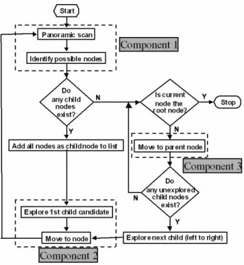
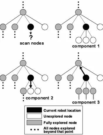
The proposed environment exploration and modeling algo-rithm consists of 3 primary components. The overall pro-cess is shown in Figure 1. The mobile robotic agent models the environment as a collection of nodes on a graph. The first component of the algorithm is to identify potential child nodes from a given location, see Figure 2. At each node the robot conducts a panoramic scan of the environment. This scan is done as a series of 2-D image snapshots using in-place rotations of the base by known angles. Next, an infor-mation theoretic metric, described in Section 3.1, is used to divide the panoramic image into regions of interest. If any region of interest has an information content above a speci-fied threshold, then it is identispeci-fied as a potential child node, which would then need to be explored.
After the list of child nodes is collated, each child node is
Figure 1: Algorithm overview.
explored sequentially. To explore a child node, the mobile agent must traverse to that node. The second component of the algorithm is to traverse to a child node from the current node (Figure 2). This is achieved by tracking the target node using a simple region growing tracker and a visual servo con-troller, using fiducial (auxiliary) points to improve accuracy. If the node cannot be reached by a straight line due to an ob-struction, then the point of obstruction is defined as the new child node. At each child node the process of developing a panoramic image, identifying the next level of child nodes, and exploring them continues.
Figure 2: Key components of the environment exploration and modeling algorithm.
the parent node pointed in the same direction, determines if the robot has reached the parent node.
These three components – imaging and evaluation, branching and retracing its steps – continue until the robot has mapped the environment to a specified level of detail. The level of detail is application-dependent and specified before the ex-ploration/mapping process is initiated. Therefore the space complexity of the algorithm can be limited by a characteris-tic parameter such as the robot size. Two nodes would then be considered as distinct whenever their distance is larger than such parameter. The set of nodes and the images taken at each node are combined into a graph to model the envi-ronment. By tracing its path from node to node, a service robot can then continue to navigate as long as there are no substantial changes to the environment (even though the pro-posed approach is relatively robust to such changes). Figure 3 shows the partial exploration of an indoor environment by a mobile robot using the IB-SLAM algorithm.
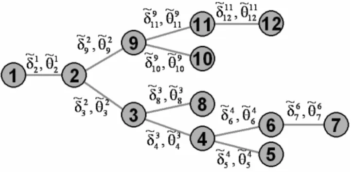
Each node on the graph consists of a panoramic scan at that node, while each branch on the graph consists of a heading and distance between the two connected nodes. The true
lo-Figure 3: Mapped environment, showing actual node loca-tions and orientaloca-tions (top view).
cation of the nodes within the environment is shown in Fig-ure 3. Note that the walls and obstacles were later added to this figure, because the robot cannot evaluate its distance from them due to the absence of range sensors or stereo cam-eras. Still, the robot can visually recognize the existence of such walls and localize itself within its surroundings using the generated nodal map. In this map, each node j is located at a distanceδijfrom its parent node i, at an angleθij(with re-spect to the original start angle). However, in this algorithm absolute distances and angles cannot be measured accurately, since they depend on odometry. Dead reckoning errors (due to wheel slip) do not allow for very accurate measurements in distance by a wheel odometer. These errors are dependent on the floor surface, so slippery surfaces would lead to larger heading uncertainties. The distance and angle of node j from its parent node i are represented by the estimates δ˜ij andθ˜ij respectively, see Figure 4. In the next sections, the details of the three key components of the algorithm are developed.
3
CHILD NODE IDENTIFICATION
cam-Figure 4: Generated graph model showing estimated node locations and orientations from Figure 3.
era (or camera field of view). The process of capturing and trimming images continues until a full 360˚ panoramic scan is achieved. Conventional image joining operations can then be used to fuse the panoramic image together. For example, two images may be joined by identifying fiducials common to both to find a transformation between them. An extensive study on the image joining techniques for mosaicing used in this work is shown in Belo (2006).
The key idea to identify potential child nodes is to reduce the acquired panoramic image using a quadtree decomposition method. In a quadtree decomposition, the image is divided into four equal quadrants. Each quadrant is evaluated to de-termine if further division of that quadrant is required based on a specific metric. In this work, the chosen metric is the information content in the image, described in the next sec-tion. This process continues until no further decomposition is required. This quadtree decomposition of the image may be used in a manner suitable to the application. Here the decom-position metric is the quantity of information in the quadrant. If the information in the quadrant exceeds a predefined value, then further decomposition is warranted. The goal of deter-mining the amount of information in the image is to identify regions where there are significant changes occurring in en-vironment. These changes would indicate the presence of a corner, an edge, a doorway, an object, and other areas worth exploring.
But highly textured surfaces (such as furniture, carpets, cur-tains, wallpaper) or noise may also be identified as regions with high information content. Clearly these are regions that need not be explored and mapped. Thus, before the quadtree decomposition process starts, the image is pre-processed to remove these high frequency effects. Pre-processing in-cludes a two step process. First, a low pass filter is applied to the image to remove the higher frequency effects. Second, an adaptive decimation process, described in Sujan et al. (2003) and Sujan et al. (2004), smoothes out patterns that exceed neighboring pattern variance. This is achieved by measuring
the rate of change of pattern variance across the image. The algorithm limits the rate of change of pattern variance within its neighborhood, by comparing pixel intensity variance in windows with respect to similar windows located in the im-mediate neighborhood (nearest neighbors). When the rate of change of pixel intensity variance exceeds a prescribed rate, then the window is gradually passed through a low pass filter until the rate of change decreases to within bounds. Cali-bration is required and it is task dependent to determine the prescribed rate of change of pixel intensity variance as well as maximum window size. Once the image has been prepro-cessed, the information content may then be evaluated.
3.1
Measures of Image Information
Con-tent
The information gained by observing a specific event among an ensemble of possible events may be described by the func-tion (Reza 1994)
H(q1, q2, ..., qn) =− n
X
k=1
qklog2qk, (1)
whereqkrepresents the probability of occurrence for thekth
event. This definition of information may also be interpreted as the minimum number of states (bits) needed to fully de-scribe a piece of data. Shannon’s emphasis was in describing the information content of 1-D signals. In 2-D, the gray level histogram of an ergodic image can be used to define a prob-ability distribution
qi =fi/Nfori= 1... Ngray, (2)
where fi is the number of pixels in the image with gray
leveli, N is the total number of pixels in the image, and Ngrayis the number of possible gray levels. With this
def-inition, the information of an image for which all theqi are
Lempel-Ziv-Welch (LZW) compression. An ideal compres-sion algorithm would remove all traces of any pattern in the data. Such an algorithm currently does not exist, however the LZW is well recognized to approach this limit. A thorough review is beyond the scope of this paper, but limited stud-ies have been carried out on several compression methods, with results presented in Sujan et al. (2006). Thus, the infor-mation content is evaluated using the compressed version of the acquired panoramic image instead of the original image. The smooth gradient example would result in a much smaller compressed file than the random image, leading to a smaller information content, as expected.
3.2
Information-Based Node
Identifica-tion
The information theory developed above is used to identify potential child nodes. The algorithm breaks down the en-vironment map into a quadtree of high information regions. The resulting image is divided into four quadrants. The infor-mation content of the compressed version of each quadrant is evaluated using Eqs. (1) and (2) and a lossless compres-sion algorithm. This information content reflects the amount of variation of the image in that quadrant (where higher in-formation content signifies higher variation in the image sec-tion). Quadrants with high information content are further divided into sub-quadrants and the evaluation process is con-tinued. This cutoff threshold of information is based on a critical robot physical parameter. This parameter can be, e.g., the wheel diameter, since terrain details much smaller than the robot wheels are irrelevant with respect to traversability. After the quadtree of the image is generated, a series of bi-nary image operations are carried out to identify the nodes. First, starting with an image template of zero intensity, the edges of every quad in the quadtree are identified and marked on in the template image. Next, the dimensions of the small-est quad are ascertained. All pixels falling within quads pos-sessing this minimum dimension are marked on in the tem-plate image. Next, an image opening operation is carried out on the template image to remove weak connectivity lines. The resulting image consists of distinct blobs. The centroids of each blob are identified as the potential nodal points. Fi-nally, the image coordinates of these nodal points are trans-ferred to the original panoramic scan to obtain the final nodal point.
The number of child nodes can be limited for each parent using a few heuristic rules - such as planar proximity - to speed up the mapping process. In addition, to avoid gener-ating child nodes at points that have already been explored, a uniqueness confirmation is carried out for every new child node identified. Given the intrinsic parameters of the cam-era, the direction of the identified child node from the current
node may be readily determined. Consequently, the direction to get back to the current node from the identified child node may be computed. The expected view from the child node in this direction may then be approximated. If any previously explored nodes have a similar view in the same direction (i.e., if both node images correlate within some user-defined toler-ance) then the identified child node is not considered unique and thus may be eliminated. The algorithm component to traverse to the unexplored child node is discussed next.
4
TRAVERSE TO UNEXPLORED NODE
The second component of the algorithm is to navigate the mobile robot to an unexplored child node from the current node. This is achieved by tracking one of the child (target) nodes obtained in the first component of the algorithm using a simple region growing tracker and a visual servo controller. The visual servo controller corrects for errors in heading of the mobile robot as it tracks the desired target. Target heading angleθis determined based on the camera focal length and the position of the target node on the imaging plane. The visual servo controller continues guiding the mobile robot until either the target node image vanishes across the image bottom (or top) edge, or the robot’s motions are ob-structed. At this point the child node is established, while its direction and odometric distance from the parent node are recorded. If the node cannot be reached by a straight line, then the point of obstruction is defined as the new child node, and the directionality of this obstruction is saved. When the child node list from Section 3 is compiled at this new node, then any nodes requiring motion in the direction of the ob-struction are eliminated from the list.
Improved accuracy may be obtained by concurrently track-ing multiple fiducials to determine the primary target head-ing, instead of tracking a single target point. This improved heading accuracy obtained through increased redundancy is a feature that can be turned on or off depending on how ac-curately one needs to move.
Let the estimated headingθ˜(computed on the imaging plane) be related to the true headingθˆby a non-linear function, h(θˆ). The measurement vector is corrupted by a sensor noise v of known variance, R:
˜
θ=h(θ)ˆ +v (3)
Hk = ∂h(θ)ˆ ∂θˆ
θˆ= ˆθ
k
(4)
The state (or computed heading) may then be estimated as follows:
Kk=PkHTk hHkPkHTk +Rki−1 ¯
θk+1= ¯θk+Kkhθ˜k−h(θˆk)i Pk+1=
1−KkHk
Pk
, (5)
where Pkis the uncertainty associated with the heading after
the kthfiducial is accounted for, and K
kis the gain associated
with the kthfiducial. This estimate is known as the Extended
Kalman Filter (Gelb 1974).
To maintain a measure of absolute error in heading of the robot at the current node with respect to the root node of the exploration tree, the uncertainty associated with each step in getting to the current node needs to be combined. This is achieved using a recursive method to determine the mean and uncertainty ofθ¯based on the previous i nodes as follows:
¯ θi+1 =
“ iθ¯
i+ ¯θi+1
”
i+1
Pθi¯+1=iP
¯ θ
i+hθ¯i
+1−
¯ ¯ θi
+1
ih
¯ θi
+1−
¯ ¯ θi
+1
iT i+1
(6)
Obtaining appropriate spatial points is now addressed. Spa-tial points are a visible set of fiducials that are tracked during sensor motion. As the sensor moves, the fiducials move rela-tive to the sensor, eventually moving out of the sensor view. This requires methods to identify and track new fiducials. While traversing to the child node, fiducials are selected au-tomatically from the image based on the visual contrast of the sampled point with its surroundings, giving a fiducial evalu-ation function (FEF) defined as:
FEF=g(C(u,v)), (7)
where g(C(u,v)) is the product of the contrast (C) and the window size (w), and contrast is defined as:
C(u,v)= I(x)¯−Iw¯
Iw , (8)
where I(x) is the 2-D image intensity value of the potential fiducial at x, I¯w is the average intensity of a window cen-tered at the potential fiducial in the 2-D image, and w is the
maximum window size after which the contrast starts to de-crease. A penalty is added if a potential fiducial is too close to other identified fiducials or too far from the tracked target. Note however that closeness of the fiducials cannot be guar-anteed because the single camera cannot provide 3-D data. Therefore, fiducials are automatically selected based on their apparent closeness in a 2-D sense. This is not an issue since fiducials are constantly being selected during the approach to the target node. Using the identified fiducials, sensor mo-tion can be identified. Fiducials can be tracked with simple methods such as region growing or image disparity corre-spondence.
Using both the measure of target heading as well as an odo-metric measure on distance traversed, the mobile robot gen-erates a graph similar to the one in Figure 4. Although these measures may be inaccurate, they serve as key parameters in estimating future movements along the graph. The process to return from a child node to its parent is described next.
5
TRAVERSE TO PARENT NODE
The third component of the algorithm is to move back to a parent node. Moving to a parent node requires a process quite different from the process of moving to an unexplored child node. The process is shown in Figure 5. It is important to note that the process described in this section is used to ap-proach any node that has been previously visited. Thus, once the map has been built, this process is used by the robot to navigate throughout the entire graph and around its environ-ment. It can be used to traverse either from child to parent or from parent to child, as long as both locations (landmarks) include previously taken panoramic images to be compared.
5.1
Identifying Parent Node Direction
Figure 5: Flow diagram to traverse to parent node.
There are several algorithms to correlate the images from the child and parent nodes. One approach is to use a polar co-ordinate representation of both images. Given a digitized bi-nary image in (x, y) coordinates along with the centroid of this image, P, a polar coordinate system can be easily gen-erated centered at P (with a maximum radius, r, equal to the maximum radius of the pixels). This image is then seg-mented both in the radial and angular directions. Counting the number of “dots” in each ring and each sector will give a radial vector Vrand angular vector Vθrespectively. If there
are M rings and N sectors in this polar coordinate, then the two vectors are M and N dimensional respectively. For sim-plicity these vectors are quantized at the integer level. Once preprocessed, the image can then be correlated to a template in order to find a match.
However, in general these acquired images may be formed relatively to the templates (rotated, scaled or trans-lated). This can be resolved by either setting up a large set
Figure 6: Image view overlap.
of templates that cover all possible transformations, or by finding an appropriate mathematical image transform that is invariant to image rotation, scale and translation. There are many different kinds of image invariants such as moment, al-gebraic and projective invariants (Casasent 1978, Ruanaidh 1997).
The use of integral transform-based invariants is a relatively simple generalization of transform domain. The number of robust invariant components is relatively large, which makes such transforms suitable for spread spectrum techniques. In addition, mapping to and from the invariant domain to the spatial domain is well-defined and it is in general not com-putationally expensive. The invariant used in this work is based on the Mellin transform, which depends on the proper-ties of the Fourier transform. Both transforms are discussed as follows.
Let the image be a real valued continuous function f(x1, x2)
defined on an integer-valued Cartesian grid with 0≤x1< N1
and 0≤x2< N2. The Discrete Fourier Transform (DFT) is
defined as F(k1, k2), where
F = N1−1
X
x1=0
N2−1 X
x2=0
f(x1, x2) exp[−i·2π(x1k1/N1+x2k2/N2)],
(9) where exp[x] is the exponential function ex. The inverse
f = 1 N1N2
N1−1 X
k1=0
N2−1 X
k2=0
F(k1, k2).
exp[i·2π(x1k1/N1+x2k2/N2)] (10)
The DFT of a real image is generally complex valued. This leads to a magnitude and phase representation for the image. This transform has several key properties, as follows. A property of the DFT is reciprocal scaling, i.e., scaling the axes in the spatial domain causes an inverse scaling in the frequency domain:
f(ρ·x1, ρ·x2)↔
1 ρF(
k1
ρ, k2
ρ) (11)
An important example of this property is the Fourier trans-form of a delta function, which has a unitrans-formly flat ampli-tude spectrum (and it is infinitely wide).
The rotation property of the DFT is such that rotating the image through an angleθ in the spatial domain causes the Fourier representation to be rotated through the same angle:
f(x1cosθ−x2sinθ, x1sinθ+x2cosθ↔ (12)
F(k1cosθ−k2sinθ, k1sinθ+k2cosθ)
Note that the grid is rotated, therefore the new grid points may not be defined. The value of the image at the nearest valid grid point may be estimated by interpolation.
Perhaps the most important property of the DFT is that shifts in the spatial domain cause a linear shift in the phase compo-nent of the transform:
f(x1+a, x2+b)↔F(k1, k2)exp[−i(ak1+bk2)] (13)
Note that both F(k1, k2)and its dual f(x1, x2)are periodic
functions, so it is implicitly assumed that translations cause the image to be “wrapped around”. This is known as a circu-lar translation. From the translation property, it is clear that spatial shifts affect only the phase representation of an image. This leads to the well-known result that the DFT magnitude is a circular translation invariant. An ordinary translation can be represented as a cropped circular translation.
However, it is less well known that it is possible to derive invariants based on the phase representation. To do this involves eliminating the translation-dependent linear term
from the phase representation. As the Taylor invariant re-moves the linear phase term in the Taylor expansion of the phase, the Hessian invariant can be used to remove this lin-ear phase term by double differentiation. In addition, prop-erties for scaling and rotation allow one to extend the basic translation invariants to cover changes of rotation and scale. This can be obtained through the Mellin Transform M(s), dis-cussed as follows.
Let us consider the scale invariant transform. For this case it is desired that:
M(f(ax)) =M(f(x)) (14)
Define the transform M(f) as follows:
M(s) = ∞
Z
0
f(x)·xs−1dx (15)
From this definition, note that the Fourier transform of f(exp ξ) is the Mellin transform M(iω)of f(x) along the imagi-nary axis of the complex plane. This relationship can be seen by the change in variables x = exp(tξ)and dx =texp(tξ)dξ. Then the above equation for the Mellin transform becomes:
M(s) = ∞
Z
0
f(x)xs−1dx=
∞
Z
−∞
f(e−ξ)e−sξdξ (16)
Substituting for s =σ+ i·2πωresults in (typicallyσ= 0):
M(iω) = ∞
Z
−∞
f(e−ξ)e−σξe−i2πωξdξ=ℑ f(e−ξ)
e−σξ
(17) For the 1-D Mellin transform, let us scale the function f(x) by a factor “a”. This gives the following result:
∞
R
0
f(ax)xiω−1dx=∞R
0
f(x) x a
iω−1dx a =
=a−iωR∞
0
f(x)xiω−1dx=a−iωM(iω)
(18)
zc=eclogz=ec(log|z|+iargz)=eclog|z|eicargz (19)
For z = a and c =tiω, it is found that arg(z) = 0 and
a−iω=e−iωlog|a|e0= cos(−ωlog|a|) +isin(−ωlog|a|)
a−iω(x+iy) =a−iω(reiθ) = =e−iωlog|a|(reiθ) =rei(θ−ωlog|a|)
(20) which corresponds only to a phase shift and not amplitude shift since|eiθ|= 1. The 2-D version of the Mellin transform
is given by:
M(ω1, ω2) =
∞ R 0 ∞ R 0
f(x, y)xi2πω1−1yi2πω2−1dxdy=
= ∞ R −∞ ∞ R −∞
f(eξ, eη)e−i2π(ω1ξ+ω2η)dξdη
(21) By back substitutingξ= tln(x) andη = tln(y) in the above equation, and noting that dξ= tdx/x and dη=tdy/y, then
M(ω1, ω2) =
∞ Z 0 ∞ Z 0 1
xyf(x, y)e
i2π(ω1lnx+ω2lny)dxdy
(22) The continuous function f(x,y) can be discretized as an N×
M matrix F with elements fk,j, where N×M is the image
size with pixel dimensions∆x and∆y, and
fk,j ≡f(k·∆x, j·∆y), (23)
with k = 1, ..., N and j = 1, ..., M. The continuous transform M(ω1,ω2) can be discretized as an U× V matrix
consid-ering frequency intervals∆u/2πand∆v/2πforω1andω2
respectively,
Mu,v≡M(u·∆u/2π, v·∆v/2π), (24)
with u = 1, ..., U and v = 1, ..., V, resulting in
Mu,v= M X j=1 N X k=1 1 k∆xe
iu∆uln(k∆x)f k,j
1 j∆ye
iv∆vln(j∆y).
(25)
The 2-D Mellin transform is then given by Tx·F·Ty, where
Tx= 1 ∆x
ei∆uln ∆x ... 1 Nei
∆ulnN∆x
ei2∆uln ∆x ... 1 Nei
2∆ulnN∆x
... ... ... eiU∆uln ∆x ... 1
NeiU
∆ulnN∆x
(26)
Ty = 1 ∆y
ei∆vln ∆y ... eiV∆vln ∆y 1
2ei
∆vln 2∆y ... 1 2eiV
∆vln 2∆y
... ... ...
1 Mei
∆vlnM∆y ... 1 MeiV
∆vlnM∆y
(27) To identify the parent node direction, a Mellin transform is used to determine whether the image that the robot currently sees is what it would expect to see if it were pointed in the correct direction toward the target node. Note however from Fig. 6 that, without any range information, the overlap di-mension of the images cannot be uniquely determined. The farther the destination node is from any wall or other fea-ture in the environment, the smaller will be the difference be-tween the views from the parent and child locations, leading to a larger overlap window. Because the robot does not have access to 3-D data, it cannot estimate its distance to the walls and therefore the scale of the overlap window. To overcome this limitation, a window growing approach is used. Here, a minimum sized overlap window is used for scale compar-ison. Progressively, this window size is increased until the correlation between the Mellin transforms of both images starts decreasing. The correlation process uses the normal-ized cross correlation RM between the Mellin transform of a
window of the observed image, M[I], and the Mellin trans-form of the expected image, M[t], to correlate them:
RM =
P
u
P
vMu,v[I]·Mu,v[t]
pP
u
P
vMu,v[I]2·pPu
P
vMu,v[t]2
(28)
This term would be maximum if the Mellin transforms of the observed and expected images were the same.
The overlap window (centered at the observed image) that yields the maximum correlation RM is then obtained, and the
correspondent value of RM stored. The robot then turns by a
small predefined angle and repeats the overlap window cor-relation process. The process goes on as the robot searches in several directions within the tolerance of the odometric heading errors. The direction that yields the maximum corre-lation RMbetween the Mellin transforms is determined to be
Figure 7: Three basic images.
Kalman Filter and odometric measures of distance/rotation, however the actual (fine) tuning of the desired direction must be done using the Mellin transform. The main reason to use dead reckoning is to speed up the process by reducing the heading search space for the Mellin transform.
As an example of correlation of Mellin transforms, consider three simple images shown in Figure 7: a white square, a cir-cle and a scaled version of the square, on a black background. Each image is 512 pixels×512 pixels. Figure 8 shows the Mellin transforms of the three images, considering∆x =∆y = 4∆u = 4∆v. Note that the Mellin transforms of both Fig-ures 8(a) and (c) are identical. It is found that the correla-tion value RM between Figs. 8(a) and (b) is 0.828, while
the one between Figs. 8(a) and (c) is exactly 1.0, the max-imum possible value. Therefore, the square and circle have a much lower correlation RM than the one for both squares,
as expected due to the invariance to scale of the Mellin trans-forms.
5.2
Approach to Parent Node
Once the direction to the parent node is established, the robot moves toward the node. Again, visual servo control based on the correlation between the current image and the image the robot would see (if it were at the parent node pointed in the same direction) governs if the robot has reached the parent node. Unlike the correlation between Mellin transforms used in the previous section, this is a correlation between the entire image observed and the one that would be expected. This process uses the normalized cross correlation between the observed image, I, and the expected image, t, to correlate them:
R=
P
k
P
jIk,j·tk,j
q P
k
P
jI 2 k,j·
q P
k
P
jt 2 k,j
(29)
The cross correlation value is then continuously evaluated as the robot moves on a straight line towards the parent node. When R starts to decrease, it is expected that the robot has reached the target node. To improve the visual servo control
Figure 8: Amplitude of the Mellin transforms of the three basic images considered.
accuracy, fiducials taken from the desired view at the parent node could also be used if correspondent ones were to be found in the current view of the robot.
reaches its local maximum. If the current heading is in the same direction of maximum RM recalculated from Eq. (28),
within a user-defined tolerance, then the robot has reached the target node. Otherwise, the robot rotates to the direc-tion of maximum RM and, assuming it is still on the line
segment connecting the child to parent nodes, the approach process resumes. This directionality verification significantly increases the robustness of the algorithm.
Finally, the robot finishes mapping the entire environment when all new potential child nodes have been explored. After that, the robot only needs to use the algorithm component 3 to travel from parent to child nodes and vice-versa within the mapped environment.
6
EXPERIMENTAL RESULTS
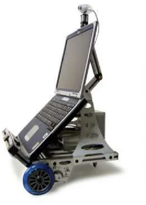
The algorithm is applied to the exploration of an apartment by a single mobile robot agent, adapted from an ER-1 com-mercial system (Evolution Robotics 2004), see Figure 9. The system consists of a 2 wheel differential system driven by step motors, equipped with wheel encoders (for odometry), three bump switches for measuring contact, and a single color camera (640×480 pixels resolution) mounted to its base. The robot is controlled by a 1.5GHz Pentium IV note-book mounted on its structure. Experimental studies were carried out in four steps. The first three steps demonstrate the validity of the three key components developed in this paper: (i) potential child node identification, (ii) traverse to unexplored child node, and (iii) traverse to parent node. The fourth step demonstrates the validity of the algorithm in de-veloping a model of its environment.
6.1
Identifying Potential Target Nodes
(Component 1)
Figure 10 shows an example of a raw image taken by the mobile agent during its exploration process. This image is trimmed and simplified using the information-based quadtree decomposition process described above. Several key areas in the image have been determined to have high quantities of in-formation present. These areas are further processed to deter-mine the coordinates of the child nodes, see Figure 11. The identification process has selected nodes that are both useful (such as the ones near the doorway), but has also picked up nodes that may not be very useful (such as the one on the carpet). These latter nodes are often eliminated with greater low pass filtering in the image pre-processing steps.
Figure 9: Mobile robot experimental system.
Figure 11: Processed image with trimmed elevation, show-ing quadtree decomposition and identified child nodes from Fig.10.
6.2
Traverse to Unexplored Child Node
(Component 2)
Figure 12 shows four steps in guiding the mobile robot to the target child node, obtained from Component 1. The node is tracked using a simple region growing method. Optionally, the correlation method described in Section 5.2 may be em-ployed. For the example shown in Figure 12, in addition to the primary target (+), two redundant fiducials are selected and tracked (O). These fiducials were selected close to the primary target. This permits fewer re-identifications of fidu-cials. However, this may result in higher inaccuracy in the visual tracking controller, since fiducials too close together would result in poorer position estimates.
6.3
Traverse to Parent Node (Component
3)
As discussed in the previous sections, heading estimates are obtained from Kalman-filtered odometric data to speed up the search process. When the robot is roughly heading in the direction of the parent node, it compares its current view with the one it would have if it were at the desired target. The robot finds the window of the current view that best cor-relates with the view from the desired location using Mellin transforms. It manages to find the correct heading by search-ing for the direction in which the best window correlation
Figure 12: Robot view while tracking to a child node (+) with the aid of fiducials (o).
Figure 13: Determining appropriate view to parent node.
is maximum. Figure 13 shows three images considered in determining the correct direction to the parent node from a child node. Figure 13(a) shows the view that the robot would see if it were at the parent node directed away from the child node, i.e., facing 180˚ from the direction of the child node. Figure 13(b) shows a view from the child node not point-ing in the correct direction to the parent node (with the robot slightly misaligned to the left). Figure 13(c) shows a view from the child node while pointing in the correct direction to the parent node.
trans-forms of Figures 13(a) and (c) is much higher than the one obtained from Figures 13(a) and (b). This can be seen by the peak value of the product Mu,v[I] and Mu,v[t], which is
2.26×10¹⁵in the first case and only 1.15×10¹⁴in the sec-ond, almost a factor of 20. It is clear from this example that the correct direction to the parent node shown in Figure 13(c) may be accurately determined.
An additional improvement can be implemented in the com-ponent 3. It has been shown that the amplitude of the Mellin transform is invariant to scale. In addition, it is well known that the amplitude of the Fourier transform is invariant to translation, while its scale is inversely proportional to the scale of the original function or image. Therefore, the Mellin transform of the amplitude of the Fourier transform of an im-age is invariant to both scale and translation. This refinement has been implemented on the experimental system, signifi-cantly improving its robustness.
These invariants work well when considering a flat-floored environment. However, even these ideal environments are subject to small image rotations caused by floor irregulari-ties. An even more robust invariant can be obtained, invari-ant to scale, translation and rotation. This can be done by means of a log-polar mapping. Consider a point (x, y)∈R2
and define
x=eµcosθ, y=eµsinθ, (30)
whereµg R and 0≤ θ < 2π. One can readily see that for every point (x, y) there is a point (µsgθ)that uniquely corresponds to it. The new coordinate system is such that both scaling and rotation are converted to translations. At this stage one can implement a rotation and scale invari-ant by applying a translation invariinvari-ant such as the Fourier transform in the log-polar coordinate system. This trans-form is called a Fourier-Mellin transtrans-form. The modulus of the Fourier-Mellin transform is therefore rotation and scale invariant.
Finally, to implement a translation, rotation and scale invari-ant, one just needs to consider the modulus of the Fourier-Mellin transform of the modulus of the Fourier transform of the image. This would improve even more the robustness of the algorithm component 3, however at the cost of a larger computational effort. For the experiments performed in this work on a flat-floored environment with good illumination, the SLAM algorithm was successfull in finding the parent nodes in all cases without the need of such additional refine-ment, see Figure 14.
6.4
Full Exploration
The results of the experimental exploration of a flat-floored apartment environment are shown in Figure 14. Each node is marked and linked to its parent/child nodes. This map may then be used for navigation by the robot within its environ-ment. Note that the walls and furniture were later added to the figure, since the absence of range sensors or stereo vision prevents the robot from identifying their exact loca-tion, unless the contact sensor is triggered during the explo-ration process. However, the robot is able to recognize its environment, including walls and furniture, from the set of panoramic images taken at each landmark. At the end, the robot does not have a standard floor plan of the environment, instead it has a very unique representation consisting solely of a graph with panoramic images taken at each node, which is enough to localize itself. This significantly reduces the memory requirements and ultimately the computational cost of such mobile robots, particularly since Mellin transforms are considerably fast and efficient. In addition, it is possible to include some human interaction during the mapping pro-cess, giving names to each environment the robot explores (such as “kitchen”, “living room”, etc.), which would im-prove the functionality of the system to be used as, e.g., a home service robot.
From the performed experiments it is found that in all cases the robot is able to localize itself, always arriving at the de-sired nodes, due to the efficiency of the Mellin transform. Note that the error in reaching a desired node is not a function of how far down the graph the node is, because the Mellin
transform will be only considering the image that the target node has in memory. However, the accuracy will be a func-tion of what the image is like, i.e., a more "busy"image will likely result in less position error as the multitude of features will help in the correlation. However, too busy an image will result in some degradation.
Additionally, if all objects in the image are quite far away, then the image will not change much as the robot moves. This will result in degradation with distance. It has been found that the positioning error of the robot is directly pro-portional to its average distance to the walls and obstacles in its field of view, and inversely proportional to the camera resolution. For twenty test runs on our experimental system in indoor environments, with distance from walls ranging in average between one and ten meters, and with a (limited) camera resolution of 176 x 144 pixels, an average ing error of 60mm (RMS) has been obtained. This position-ing accuracy can certainly be improved with a better camera resolution.
7
CONCLUSIONS
In this work, an information-based iterative algorithm has been presented to plan the visual exploration strategy of an autonomous mobile robot to enable it to most efficiently build a graph model of its environment using a single base-mounted camera. The algorithm is based on determining the information content present in sub-regions of a 2-D panoramic image of the environment as seen from the cur-rent location of the robot. Using a metric based on Shan-non’s information theory, the algorithm determines potential locations of nodes from which to further image the environ-ment. Using a feature tracking process, the algorithm helps navigate the robot to each new node, where the imaging pro-cess is repeated. A Mellin transform and tracking propro-cess is used to guide the robot back to a previous node, using pre-viously taken panoramic images as a reference. Such inte-gral transform has the advantage of being able to efficiently handle environments with high information content, as op-posed to other localization techniques that rely, e.g., on find-ing corners in the image. However, Mellin transforms lose efficiency in dynamic environments. In these cases, other in-variant transforms such as SIFT (Se et al. 2002) would be recommended. Finally, the imaging, evaluation, branching and retracing its steps continues until the robot has mapped the environment to a pre-specified level of detail. The set of nodes and the images taken at each node are combined into a graph to model the environment. By tracing its path from node to node, a service robot can navigate around its environ-ment. This method is particularly well suited for flat-floored environments. Experimental studies have been conducted to demonstrate the effectiveness of the entire algorithm. It was
found that this algorithm allows a mobile robot to efficiently localize itself using a limited sensor suite (consisting of a single monocular camera, contact sensors, and an odometer), reduced memory requirements (only enough to store one 2-D panoramic image at each node of a graph), as well as modest processing capabilities (due to the computational efficiency of Mellin transforms and the proposed information-based al-gorithm). Therefore, the presented approach has a potential benefit to significantly reduce the cost of autonomous mobile systems such as indoor service robots.
REFERENCES
Alata, O., Cariou, C., Ramananjarasoa, C., Najim, M. (1998). Classification of rotated and scaled textures us-ing HMHV spectrum estimation and the Fourier-Mellin transform.Proceedings of the International Conference on Image Processing, ICIP 98, vol. 1, pp.53-56. Anousaki, G.C. and Kyriakopoulos, K.J. (1999).
Simultane-ous localization and map building for mobile robot nav-igation.IEEE Robotics & Automation Magazine, vol. 6, n. 3, pp.42-53.
Belo, F.A.W. (2006). Desenvolvimento de Algoritmos de Ex-ploração e Mapeamento para Robôs Móveis de Baixo Custo. M.Sc. Thesis, Dept. Electrical Engineering, PUC-Rio, in portuguese.
Borenstein, J. and Koren, Y. (1990). Real time obstacle avoidance for fast mobile robots in cluttered environ-ments.IEEE International Conference on Robotics and Automation, pp.572-577.
Casasent, D., Psaltis, D. (1978). Deformation invariant, space-variant optical pattern recognition.Progress in optics, vol.XVI, North-Holland, Amsterdam, pp.289-356.
Castellanos, J.A., Martinez, J.M., Neira, J. and Tardos, J.D. (1998). Simultaneous map building and localization for mobile robots: a multisensor fusion approach.IEEE International Conference on Robotics and Automation, vol. 2, pp.1244-1249.
Evolution Robotics (2006). Webpage www.evolution.com, last access May 12, 2006.
Gelb, A. (1974). Applied optimal estimation. MIT press, Cambridge, Massachusetts, U.S.A.
Kruse, E., Gutsche, R. and Wahl, F.M. (1996). Efficient, iter-ative, sensor based 3-D map building using rating func-tions in configuration space.IEEE International Con-ference on Robotics and Automation, vol. 2, pp.1067-1072.
Lavery, D. (1996). The Future of Telerobotics. Robotics World, Summer 1996.
Lawitzky, G. (2000). A navigation system for cleaning robots.Autonomous Robots, vol. 9, pp.255-260. Leonard, J.J. and Durrant-Whyte, H.F. (1991). Simultaneous
map building and localization for an autonomous mo-bile robot.IEEE International Workshop on Intelligent Robots and Systems, vol. 3, Osaka, Japan, pp.1442-1447.
Reza, F.M. (1994). An introduction to information theory. Dover, New York.
Ruanaidh, J.O. and Pun, T. (1997). Rotation, scale and trans-lation invariant digital image watermarking.IEEE In-ternational Conference on Image Processing(ICIP 97), Santa Barbara, CA, U.S.A., vol. 1, pp.536-539. Se, S., Lowe, D.G., Little, J. (2002). Mobile robot
localiza-tion and mapping with uncertainty using scale-invariant visual landmarks. International Journal of Robotics Re-search, vol.21, n.8, pp.735-758.
Simhon, S. and Dudek, G. (1998). Selecting targets for lo-cal reference frames.IEEE International Conference on Robotics and Automation, vol.4, pp.2840-2845. Sujan, V.A., Dubowsky, S., Huntsberger, T., Aghazarian,
H., Cheng, Y. and Schenker, P. (2003). Multi Agent Distributed Sensing Architecture with Application to Cliff Surface Mapping.11th International Symposium of Robotics Research(ISRR), Siena, Italy.
Sujan, V.A., Meggiolaro, M.A. (2005). Intelligent and Ef-ficient Strategy for Unstructured Environment Sensing using Mobile Robot Agents.Journal of Intelligent and Robotic Systems, vol. 43, pp.217-253.
Sujan, V.A., Meggiolaro, M.A. (2006). On the Visual Ex-ploration of Unknown Environments using Informa-tion Theory Based Metrics to Determine the Next Best View. In: Mobile Robots: New Research, Editor: John X. Liu, NOVA Publishers, USA.
Thrun, S. (2003). Robotic mapping: a survey. In: Exploring artificial intelligence in the new millennium, Morgan Kaufmann Publishers Inc., San Francisco, CA, USA, pp.1-35.
Thrun, S., Burgard, W. and Fox, D. (2000). A retime al-gorithm for mobile robot mapping with applications to multi-robot and 3D mapping.IEEE International Con-ference on Robotics and Automation, vol. 1, pp.321-328.
Thrun, S., Burgard, W., Fox, D. (2005). Probabilis-tic RoboProbabilis-tics (Intelligent Robotics and Autonomous Agents). MIT press, Cambridge, Massachusetts, U.S.A. Tomatis, N., Nourbakhsh, I. and Siegwar, R. (2001). Simul-taneous localization and map building: a global topo-logical model with local metric maps.IEEE/RSJ Inter-national Conference on Intelligent Robots and Systems, vol. 1, pp.421-426.
Wong, S., Coghill, G. and MacDonald, B. (2000). Natu-ral landmark recognition using neuNatu-ral networks for au-tonomous vacuuming robots. 6th International Con-ference on Control, Automation, Robotics and Vision,