Meshless methods in electromagnetic wave scattering

(1)

Universidade Federal de Minas Gerais

Programa de Pós-Graduação em Engenharia Elétrica

Escola de Engenharia

Meshless Methods in Electromagnetic Wave Scattering

Williams Lara de Nicomedes

(2)

(3)

(4)

(5)

v

By nature, all men long to know.

(6)

vi

(7)

vii

Abstract

(8)

viii

Resumo

(9)

ix

Acknowledgements

This work could not have been brought to its full completion without the contributions of the individuals below. Each one gave a parcel of what proved to be absolutely fundamental to the production of this dissertation. They are:

Prof. Fernando Moreira, who gave me the opportunity to join his research group, and who willingly has arranged me scholarships (since the time I was an undergraduate!);

Prof. Renato Mesquita, who introduced me to the field of meshfree analysis (and this happened in a most unexpected way, since originally my research purposes were aimed at another direction);

Prof. Cassio Rego and Prof. Odilon Filho, who, through their classes, gave me a more profound knowledge of electromagnetic theory, so necessary for this work;

Prof. Reinaldo Palhares and all the CPDEE staff, who provided all the support for the academic activities throughout the Master’s course.

(10)

x

Agradecimentos

Este trabalho não poderia ter alcançado um patamar satisfatório sem a contribuição dos indivíduos listados abaixo. Cada um deu uma parcela que se revelou absolutamente fundamental para a produção desta dissertação. São eles:

Prof. Fernando Moreira, que permitiu que eu me associasse a seu grupo de pesquisa, e que benevolamente me tem conseguido bolsas de estudo (desde o tempo em que eu era um estudante de graduação!);

Prof. Renato Mesquita, que me apresentou ao campo de estudo dos métodos sem malha (e isso aconteceu de uma maneira totalmente inesperada, visto que primeiramente meus interesses de pesquisa estavam direcionados para um outro rumo);

Prof. Cássio Rego e Prof. Odilon Filho, que através de suas aulas, me proporcionaram acesso um conhecimento mais profundo sobre teoria eletromagnética, tão necessário para este trabalho);

Prof. Reinaldo Palhares e toda a equipe do CPDEE, que ofereceram todo o apoio para a realização das atividades acadêmicas durante o curso de mestrado.

(11)

xi

Resumo Estendido

Introdução

s métodos sem malha (geralmente referenciados pelas expressões meshless ou meshfree) são uma família de procedimentos computacionais destinados à solução numérica de equações diferenciais parciais. Operacionalmente, tais métodos realizam as mesmas tarefas que métodos mais tradicionais, como o método de elementos finitos (FEM) e o método de diferenças finitas (FDTD), entre outros. Isto é, dada uma equação diferencial parcial, os métodos sem malha são aptos (ou pelo menos deveriam ser) a fornecer uma solução numérica para essa equação, da maneira mais acurada possível. Mas esses métodos resolvem equações de uma maneira bastante peculiar, baseando-se numa característica tão distinta que ela acabou por dar nome à inteira família de métodos: a completa ausência de malhas.

Mas o que viria a ser isso? O que seria uma malha? De maneira bastante informal (e sem qualquer intenção de expor definições e raciocínios rigorosos), uma malha seria uma subdivisão do domínio no qual uma dada equação deve ser resolvida. Uma equação diferencial deve ser satisfeita num domínio , i.e., uma porção limitada do espaço uni, bi ou tridimensional.

Ao se resolver essa equação num computador, os métodos tradicionais “quebram” o domínio

numa coleção de pedaços menores. O domínio pode ser subdividido de maneira regular, como no caso do FDTD, dando origem a uma malha estruturada, ou de maneira irregular (mas obviamente obedecendo a critérios específicos), originando uma malha irregular, prática comum no FEM.

Os métodos sem malha, por outro lado, não trabalham com subdivisões do domínio. Uma vez que é definido, espalha-se sobre ele um conjunto de pontos (chamados de nós), aos quais se associam certas funções, conhecidas como funções de forma (ou de base). A solução da equação para qualquer ponto é então calculada como uma soma ponderada de funções de forma calculadas em . Em suma, isso seria a essência dos métodos sem malha. Não parece muito complicado, mas há um longo caminho a percorrer para se achar os pesos da soma ponderada citada acima. Há diversas maneiras de se calculá-los, cada uma dando origem a um diferente método (estamos a falar de uma família de métodos). Alguns são mais formidáveis do que outros, é claro, mas todos compartilham dessa mesma filosofia, que, aliás, é o tema do capítulo 2 dessa dissertação.

Os primeiros estudos a respeito dos métodos sem malha datam do início da última

década. Ainda estão na sua “infância”, e ainda há muitos desafios que precisam ser explorados

(12)

xii

Dentre os membros da família, um em particular, o EFG (Element-Free Galerkin) tem sido empregado com sucesso [Parreira et al., 2006], [Bottauscio et al., 2006] e [Manzin e Bottauscio, 2008]. Entretanto, o EFG não é considerado como um método “verdadeiramente” sem malha pelo fato de depender de um procedimento que lembra muito uma divisão de domínio (e portanto uma malha!) durante o processo de cálculo [Liu, 2003]. Principalmente por causa disso, o principal objetivo desse trabalho é dissecar um outro método, o MLPG (Meshless Local Petrov-Galerkin), e tentar encontrar o maior número possível de aplicações a problemas tradicionais da engenharia elétrica. O MLPG, desenvolvido inicialmente por S. Atluri [Atluri and Shen, 2002] é verdadeiramente sem malha, e utiliza informações relativas à vizinhança de cada nó para se chegar à solução geral do problema. Ele parte do local (a versão do MLPG explorada neste trabalho emprega vizinhanças circulares em 2D e esféricas em 3D) para o global. Uma abordagem muito interessante, que será explicada um pouco mais nas próximas linhas (e no restante do trabalho).

Funções de Forma

De acordo com o que foi explicado acima, a principal noção que permeia os métodos sem malha é a aproximação da solução por uma soma ponderada de funções de forma (associadas a nós espalhados pelo domínio, e não a elementos). Dado um ponto pertencente ao domínio , tem-se:

em que:

é a versão discretizada (i.e., representada como uma soma de funções de forma) da solução da equação diferencial parcial a ser resolvida numericamente ( é um operador diferencial e uma função conhecida, não necessariamente contínua);

representa o conjunto de nós que são aptos a influenciar o ponto ;

representa uma função de forma associada ao nó calculada em ;

é o parâmetro nodal, i.e., o peso associado ao nó .

A noção geométrica associada à equação (1) acima é mostrada na Fig.3.1.

Dentre as propriedades que as funções de forma devem satisfazer, estão:

1 - Devem ser de suporte compacto (i.e., possuem valor diferente de zero apenas na vizinhança do nó ao qual está associada). Isso garante que somente os nós mais próximos do ponto onde se deseja calcular contribuem com a soma ponderada (1). Essa característica leva naturalmente a sistemas lineares cujas matrizes são esparsas, de maneira análoga ao FEM;

2 - Todas as funções de forma que influenciam um ponto devem satisfazer a partição da

(13)

xiii

e também a propriedade da reprodução do campo linear:

As expressões (2) – (5) informam que as funções de forma conseguem aproximar uma função linear de maneira exata, i.e., se é sabido de antemão que a solução de uma equação diferencial é linear, então o erro cometido ao se aproximar a função pela sua versão discretizada é zero.

Há diferentes maneiras de se calcular as funções de forma . E aqui talvez resida o ponto fraco dos métodos sem malha. As funções de forma não possuem expressão analítica. Diferentemente do FEM, onde as funções de base são conhecidas no interior de cada elemento, os métodos sem malha requerem a aplicação de métodos numéricos para sua determinação. Na abordagem meshless, pode-se dizer que o custo computacional para se construir uma malha não-estruturada é transferido para o cômputo das funções de forma.

Na quase totalidade dos problemas avaliados neste trabalho, a aproximação MLS (Moving Least Squares) foi empregada [Liu, 2003]. Funções de forma RPIM [Liu, 2003] foram empregadas apenas uma vez, na seção 5.4).

As funções de forma MLS se apoiam basicamente na geometria da distribuição nodal (i.e., posição dos nós no domínio ) e no domínio de influência associado aos nós:

 Cada nó é associado a um número real (problemas unidimensinais), a um par ordenado (bidimensionais), ou a uma trinca ordenada (tridimensionais), que localiza o nó no interior (ou na fronteira) do domínio ;

 As funções de forma são capazes de influenciar (i.e., são diferentes de zero) apenas uma região na vizinhança de cada nó (apenas uma outra maneira de se dizer que as funções de forma são de suporte compacto). Há uma certa liberdade na escolha da forma dessas regiões. Neste trabalho, elas são círculos em 2D e esferas em 3D.

Portanto, para cada nó (índice que varia de 1 a , número total de nós espalhados por ) localizado em , tem-se uma uma função de forma que assume valores diferentes de zero na região

(14)

xiv

em que é o raio da região (circular ou esférica) . Visto que apenas os pontos que se situam no interior de podem ser influenciados pelo nó , recebe o nome de domínio de

influência associado ao nó .

Uma vez que a noção de influência tornou-se mais precisa através de (2), uma interpretação mais refinada de (1) seria: Dado o ponto no qual se deseja calcular , toma-se toda a população nodal (índices de 1 a ) e considera-se apenas aqueles para os quais (i.e., o nó influencia ). Esses nós formam o conjunto . Mas e se porventura houvesse um ponto para o qual ? Como se poderia construir uma aproximação para ? Na verdade, tal cenário é inconsistente; o ponto estaria dentro de um ‘buraco de

cobertura’. Se a abordagem meshless deve ter algum sentido para todos os pontos do domínio , precisa-se garantir que

i.e., os domínios de influência de todos os nós devem formar uma cobertura para o domínio (e para a sua fronteira ).

O processo para se calcular as funções de forma MLS é longo e tedioso. O Capítulo 3 é quase inteiramente devotado a ele. Nesta breve introdução, é suficiente dizer que, dado um ponto no qual se deseja calcular as funções de forma, tem-se:

em que

( significa o primeiro elemento do conjunto , o segundo, e assim por diante, até o número de nós que influenciam o ponto ; uma descrição detalhada do que realmente está por trás de e é dada no Capítulo 3, Seção 1). O procedimento

para se calcular as funções de forma pode ser encarado como uma ‘caixa-preta’, i.e., informa-se as coordenadas do ponto e obtém-se como resultado um conjunto de funções de forma (5) pronto a ser utilizado em aproximações de como em (1). O custo computacional associado é elevado, visto que, para cada ponto onde se deseja calcular as funções de forma, é fundamental o emprego de um algoritmo de busca (p.ex., baseado em KdTrees), além de inversões matriciais (apenas a aproximação MLS precisa de matrizes invertidas; tal procedimento é desnecessário no RPIM). O processo para o cálculo das derivadas parciais também pode ser considerado como

uma ‘caixa-preta’. Neste caso, os cálculos vão um pouco mais além, e o procedimento retorna vetores como em (5), mas contendo os valores das derivadas das funções de forma associadas aos nós que influenciam o ponto (Capítulo 3, Seção 3).

(15)

xv

Equações Integrais de Espalhamento Eletromagnético: Uma Primeira

Aplicação para as Funções de Forma MLS

Embora os métodos sem malha terem sido originalmente propostos como uma alternativa ao método dos elementos finitos (FEM), que busca a solução de equações diferenciais parciais, a primeira oportunidade neste trabalho de aplicação das funções de forma veio de um campo totalmente diferente, a saber, da análise do espalhamento de ondas eletromagnéticas através de equações integrais.

As equações integrais da teoria eletromagnética geralmente são resolvidas através do método dos momentos (MoM) [Balanis, 1989], [Harrington, 1968]. Neste trabalho, o MoM foi adaptado de tal modo a empregar as funções de forma MLS no processo de discretização.

Na análise do espalhamento de ondas por objetos condutores (a única categoria aqui considerada), busca-se uma maneira de se determinar as correntes equivalentes que são induzidas na superfície do condutor, representado por (embora de acordo com o Capítulo 1 o mesmo símbolo também seja empregado para a fronteira do domínio onde uma equação diferencial deve ser resolvida, não há nenhum problema em empregá-lo também na abordagem via equações integrais, uma vez que aqui representa a ‘fronteira’, ou o contorno do objeto condutor, onde circulam as correntes equivalentes). Para problemas bidimensionais e polarização TMz, tem-se

A equação (6) é a equação integral do campo elétrico (EFIE), e (7) é a equação integral do campo magnético (MFIE). Os campos incidentes (componente ) e são funções conhecidas, assim como a geometria da superfície do condutor (em problemas 2D, uma curva fechada em ). Uma completa dedução de (6) e (7) a partir das equações de Maxwell é dada na Seção 4.1.2.

O processo que leva à solução de (6) e (7) pode ser sucintamente descrito por:

 Espalha-se nós por todo o contorno ;

 Uma vez que as posições nodais tenham sido estabelecidas, constrói-se funções de forma MLS de acordo com o procedimento ‘caixa-preta’ (seção anterior);

 Aproxima-se a densidade de corrente por uma soma ponderada de funções de forma [à maneira de (1)]:

(16)

xvi

 Substitui-se (8) em (6) e/ou (7) e realiza-se as integrações numéricas ao longo de . Isso leva a um sistema linear cujas incógnitas são os parâmetros nodais e cujo vetor é uma função do campo incidente (e portanto conhecido).

A qualidade dos resultados obtidos depende da geometria do condutor. Tal método se revelou preciso quando aplicado ao problema de espalhamento por um cilindro circular

condutor perfeito. Entretanto, quando a seção reta do cilindro possui ‘lados’ (um quadrado, por

exemplo), o método falha miseravelmente, porque a aproximação MLS não consegue produzir as funções de forma. Se os nós estiverem distribuídos ao longo de um lado do quadrado (de modo que uma de suas coordenadas, ou , tenha um valor fixo), a matriz em (4) torna-se singular, o que impede que seja invertida.

Uma maneira de se contornar esse problema seria o emprego de um outro método para a construção de funções de forma, e que fosse apto a produzir resultados aceitáveis quando os nós estivessem distribuídos ao longo de uma linha (ou lado). A Seção 4.3 lida com o método IMLS (Improved Moving Least Squares), que emprega uma espécie de ortogonalização de Gram-Schmidt para a construção de funções para a base do MLS (vetor ). O procedimento IMLS não necessita de inversão de matrizes, e produz bons resultados longe das quinas do cilindro condutor. O IMLS falha próximo aos vértices (ou quinas), o que resulta em um desempenho não muito satisfatório.

Entretanto, há uma maneira de se resolver as equações integrais (6) e (7) através de funções de forma MLS, tanto para geometrias circulares quanto para as que contém lados. A idéia é construir as funções de forma ao longo de uma linha, e depois definir uma transformação que mapeia os pontos dessa linha a pontos do contorno . Esse processo funciona muito bem (Seção 4.4), e a ele foi dado o nome de rubber band technique, pelo fato de se parecer com o ato de esticar uma tira de borracha (que supostamente conteria as funções de forma) ao longo do contorno .

O Método MLPG (Meshless Local Petrov-Galerkin)

O MLPG é o ponto central do presente trabalho, particularmente a sua aplicação a problemas de espalhamento eletromagnético. Esse método foi desenvolvido por S. Atluri [Atluri e Shen, 2002], inicialmente para a resolução de problemas modelados por equações diferenciais parciais em Mecânica Computacional. Esse método é considerado ‘verdadeiramente’ sem malha, uma vez que requer a integração de formas fracas apenas em domínios locais, na vizinhança de cada nó.

Em problemas de espalhamento de ondas eletromagnéticas monocromáticas em duas dimensões, as equações a serem resolvidas geralmente assumem a forma

(17)

xvii

refere ao número de onda no espaço livre, e é um termo que representa as fontes (excitação).

No MLPG, a equação (9), que envolve derivadas de segunda ordem da função , não é resolvida diretamente; ela precisa ser antes colocada sob uma outra forma, a forma fraca, que envolve apenas derivadas de primeira ordem (enquanto (9) é conhecida como a forma forte do problema). Entretanto, a construção da forma fraca de (9) requer a introdução de um outro tipo de função, as funções de teste . O processo geral de solução da equação (9) via MLPG pode ser descrito como:

 Espalha-se nós através de todo o domínio ;

 A cada um dos nós se associa uma função de forma MLS ;

 A cada um dos nós se associa uma função de teste . As funções de teste também devem ser de suporte compacto (assim como as funções de forma). A região na vizinhança do nó sobre a qual é diferente de zero é chamada de domínio de teste ;

 Constrói-se a forma fraca de (9), usualmente uma expressão integral envolvendo e . A forma fraca é imposta vezes, cada uma das quais devendo ser integrada em ;

 Em cada instância da forma fraca obtida de (9), substitui-se pela aproximação (1). Tal procedimento leva a um sistema linear cuja matriz é esparsa, e cujas incógnitas são os parâmetros nodais .

Na versão do MLPG empregada neste trabalho, uma típica função de teste associada ao nó é tal que

Em duas dimensões, é dada por

E em três dimensões,

em que é o raio do domínio de teste , que deve obrigatoriamente ser um círculo em problemas 2D (e esferas em problemas 3D), nessa versão apenas, conhecida como MLPG4 ou

Local Boundary Integral Equation Method (LBIE).

No que diz respeito à forma fraca, há pelo menos duas maneiras de obtê-las: o método dos resíduos ponderados ou através da segunda identidade de Green. Uma vez que a forma fraca tenha sido obtida, ela requer a incorporação das condições de contorno, especificadas sobre a fronteira . Como se trata de problemas de espalhamento, busca-se condições que representem o campo espalhado se afastado do objeto (outward travelling waves), i.e., as condições devem satisfazer, pelo menos num sentido aproximado, a condição de Sommerfeld:

(18)

xviii

em que representa a componente do campo elétrico espalhado (as condições para o campo magnético são análogas). Neste trabalho, foram empregadas as condições de contorno de radiação (Radiation Boundary Conditions - RBC) de Bayliss-Turkel de primeira (Seção 5.5) e de segunda ordem (Seção 5.3).

As condições de radiação podem ser impostas de duas maneiras: Diretamente na forma fraca (Seção 5.3) ou através do método da colocação (Seção 5.5). A primeira alternativa apresenta um desafio maior, visto que interseções entre o domínio e os domínios de teste dos nós próximos a precisam ser encontradas. Já a segunda é muito simples de ser implementada, o que a torna mais eficiente. Ainda existe uma maneira de se lidar com (14), mas

que não emprega RBC’s aproximadas. Trata-se do método de expansão em autofunções, ou método Unimoment (Seção 5.4). Tal método foi originalmente proposto para a solução de problemas de espalhamento via elementos finitos [Chang e Mei, 1976]. Entretanto, ele foi aqui modificado de modo a incorporar o MLPG4/LBIE no lugar do FEM, com resultados bastante favoráveis.

Condições de Interface

Uma outra questão abordada neste trabalho diz respeito às condições de interface, que devem ser impostas quando algum parâmetro material [função em (9)] é descrito por uma função descontínua. Essa questão é particularmente importante na análise do espalhamento de ondas eletromagnéticas com polarização TEz. Para essa polarização, e se o domínio for caracterizado por dois (ou mais) materiais com diferentes permissividades, ao longo da interface entre os dois materiais, as derivadas normais do campo magnético satisfazem à relação

em que representa o campo magnético de uma lado da interface, enquanto é o campo do outro lado; é a permissividade relativa de um lado da interface, enquanto é a permissividade do outro lado. As derivadas em (15) são tomadas na direção normal à interface que separa os meios de permissividades diferentes. Não há uma maneira de inserir (15) diretamente na expressão para a forma fraca de (9). Entretanto, a Seção 5.5.1 apresenta um procedimento muito conveniente de tratar esse problema. As condições de interface são impostas diretamente no sistema matricial, via colocação, de um modo similar ao qual as condições de fronteira são impostas no contorno . A idéia por trás desse procedimento foi inspirada por [Li et al., 2003]. Resultados adicionais da aplicação dessa técnica a um problema tridimensional de eletrostática podem ser vistos na Seção 6.1.

Problemas de Autovalor: Cristais Fotônicos

Na análise de cristais fotônicos, há grande interesse na determinação da estrutura de

bandgap. Tal estrutura diz respeito às frequências com as quais ondas eletromagnéticas (luz)

(19)

xix

modos propagantes é um problema de autovalor; para cristais bidimensionais e assumindo ondas incidentes com polarização TMz, o problema a ser resolvido é:

sujeito às condições de contorno

em que é um vetor ligado às transformações de simetria do cristal (lattice vector). O problema (16)-(18) deve ser resolvido numa célula unitária . (Os cristais fotônicos são estruturas periódicas. A menor unidade que, quando transladada dá origem ao cristal original, é geralmente chamada de célula unitária). Neste trabalho, considerou-se apenas células unitárias quadradas. As condições (17) e (18), impostas na fronteira de uma célula quadrada significam que o campo em um lado é igual ao campo no lado oposto, multiplicado por um fator de fase (no qual o vetor é o vetor de Bloch). O mesmo vale para a derivada normal do campo elétrico.

Para se resolver o problema (16) – (18), o campo elétrico geralmente é representado como o produto de duas funções (teorema de Bloch):

onde é agora uma função periódica na célula unitária, i.e.,

A substituição de (19) em (16) dá origem a uma nova equação diferencial:

(20)

xx

Algumas Aplicações do MLPG em Mecânica Quântica

No mesmo espírito das seções anteriores, busca-se aqui soluções para problemas de autovalor provenientes da equação de Schrödinger em 2 e 3 dimensões

Basicamente, dada uma distribuição de energia potencial ( ), as Seções 7.2 e 7.3 ilustram como encontrar os níveis de energia (autovalores) . Todo o tratamento teórico é apresentado com detalhe, particularmente as estratégias para a construção da forma fraca da equação de Schrödinger a partir de (23). Comparações com os resultados de soluções analíticas demonstram a aplicabilidade do MLPG em problemas de mecânica quântica. O procedimento para construção de funções de forma periódicas do Capítulo 6 é aqui estendido com facilidade para três dimensões, para a resolução de um problema de determinação da estrutura de banda de sólidos (similar ao problema 2D para cristais fotônicos). Os resultados concordam muito bem com aqueles provenientes de um outro método numérico [Jun, 2004].

Por fim, a última seção do Capítulo 7 faz referência às primeiras incursões no emprego do MLPG4/LBIE em problemas dependentes do tempo. O objetivo é resolver a equação de Schrödinger não-linear dependente do tempo

Na abordagem aqui empregada, a derivada temporal é discretizada através de um procedimento via diferenças finitas. Além disso, ao termo não-linear é dispensado um tratamento especial, baseado em iterações (predictor-corrector). Os resultados concordam muito bem com as soluções analíticas, e revelam que o MLPG4/LBIE também funciona corretamente ao ser aplicado a problemas que dependam do tempo.

Conclusões

O trabalho aqui apresentado cumpriu o seu papel de demonstrar a aplicabilidade dos métodos sem malha a vários problemas de interesse para a engenharia elétrica. Procurou-se demonstrar com clareza como os métodos funcionam. O custo de tal empreitada refletiu-se em exposições talvez demasiado longas, principalmente naquelas referentes à construção das formas fracas.

(21)

xxi

A construção das funções de forma é o tema do Capítulo 3. A aproximação MLS foi dissecada de uma maneira particularmente incisiva, com páginas e mais páginas demonstrando o processo por trás das funções de forma MLS. Apesar de poder ser encarado como um procedimento caixa-preta, muito insight pode ser obtido caso se conheça com detalhe como essas funções de forma são calculadas. O Capítulo 3 também faz uma breve referência às funções de forma RPIM, visto que são empregadas apenas uma única vez em todo o trabalho.

Uma vez que as funções de forma – componentes básicos na aproximação dos campos – foram definidas, prosseguiu-se na aplicação dessas funções ao processo de discretização de equações integrais do espalhamento eletromagnético. Os resultados foram muito bons, superando em precisão o método dos momentos, que é tradicionalmente empregado nessa categoria de problemas. Além disso, o Capítulo 4 discute as principais falhas do MLS na

construção de funções de forma para objetos ‘quadrados’. Após muita discussão, uma maneira

extremamente simples para resolver os problemas do MLS é apresentada ao final do capítulo.

O Capítulo 5, que trata de todo o desenvolvimento do MLPG aplicado a problemas de espalhamento, é o ponto central do trabalho. Diferentes estratégias para lidar com a imposição das condições de contorno foram abordadas. O método da colocação assume aí um destaque, em vista da facilidade com a qual pode ser efetivamente empregado.

Com a experiência dos capítulos anteriores, procede-se então a novas áreas de aplicação do MLPG a problemas tridimensionais (nos quais o método da colocação uma vez mais se revelou fundamental) e a problemas de autovalor provenientes da análise de cristais fotônicos e da mecânica quântica. Esse material, tema dos últimos dois capítulos, conclui a dissertação.

A principal intenção deste trabalho foi mostrar como o MLPG pode ser aplicado a problemas de espalhamento eletromagnético. O restante deve ser encarado como ‘subprodutos’ (byproducts), que foram obtidos à medida em que o tema principal era desenvolvido. Muitos temas foram aqui tratados pela primeira vez, e particular atenção foi devotada à exposição detalhada dos métodos. Isso levou, como já afirmado, a discussões um tanto prolongadas e a deduções que à primeira vista poderiam parecer desnecessárias. Mas isso já estava previsto; uma das intenções que tive ao produzir esse trabalho é que ele também servisse como uma espécie referência, onde tudo (ou quase) o que eu tivesse explorado sobre os métodos sem malha estivesse contido.

Uma vez que a aplicabilidade dos métodos sem malha a problemas foi demonstrada com sucesso, o próximo passo é o refinamento desses métodos. Resultados sobre erros, taxas de convergência e, sobretudo, comparações extensivas com o método dos elementos finitos, constarão na agenda dos trabalhos futuros. A fronteira foi aberta, e agora pode-se vislumbrar vários temas a serem abordados, como

 Problemas que envolvam grandezas vetoriais, e não apenas escalares;

 Problemas não-lineares (principalmente aqueles relacionados à não-linearidade de certos cristais fotônicos);

 Outras maneiras de se resolver problemas dependentes do tempo;

 Uso de PML’s (Perfectly Matched Layers) ao invés de condições de radiação (RBCs’);

(22)

xxii

 Um tratamento matemático mais rigoroso (descrição mais detalhada dos espaços de funções e operadores que figuram nos métodos sem malha).

(23)

xxiii

List of Symbols

th unknown coefficient (MLS approximation, page 18)

unknown coefficients collected into a vector (MLS approximation, page 21)

one of the matrices involved in the MLS approximation (page 24)

time-harmonic magnetic potential vector – spatial part (page 43)

one of the matrices involved in the MLS approximation (page 25)

speed of light in vacuum (page 117)

auxiliary real functional (MLS approximation, page 21)

time-dependent magnetic flux density (page 37)

time-harmonic magnetic flux density – spatial part (page 39)

time-dependent electric flux density (page 37)

time-harmonic electric flux density – spatial part (page 39)

time-dependent electric field intensity (page 37)

time-harmonic electric field intensity – spatial part (page 39) th energy level (page 130)

z-component of the electric field – time-harmonic regime (page 71)

reduced Planck’s constant (page 129)

time-dependent magnetic field intensity (page 37)

time-harmonic magnetic field intensity – spatial part (page 39)

zero-order Hankel function of the second type (page 44)

_{p-order Hankel function of the second type (page 85)}

z-component of the magnetic field – time-harmonic regime (page 72) imaginary number (page 39)

time-dependent electric current density (page 37)

time-harmonic electric current density – spatial part (page 39)

time-dependent electric surface current density (page 39)

(26)

xxvi

the Bloch vector (page 117)

natural logarithm (page 76)

the lattice vector (page 117)

outward unit vector normal to a surface (page 38)

index set which collects the indices of all nodes able to influence point (page 10)

th term in the monomial basis (MLS approximation, page 18)

all monomial terms collected into a vector (MLS approximation, page 18)

one of the matrices involved in the MLS approximation (page 24) radius of the influence domain associated to node (page 19) radius of the test domain associated to node (page 75) scalar function (in or ) to be approximated (page 6) discretized version of (page 9)

nodal parameter associated to node (page 10)

vector collecting all nodal parameters (page 25) test function associated to node (page 75)

a point in or (page 6)

weight (or window) function (MLS approximation, page 19)

diagonal matrix involved in the MLS approximation (page 24)

unit vector pointing at the z-direction (page 45) test domain associated to node (page 74)

Boundary of the test domain associated to node (page 75)

auxiliary vector employed in the derivatives of MLS shape functions (page 32)

Kronecker delta (page 30)

electric permittivity (page 37) magnetic permeability (page 38) electric conductivity (page 38)

influence domain associated to node (page 10)

boundary of the influence domain associated to node (page 11)

time-dependent electric charge density (page 37)

time-harmonic electric charge density – spatial part (page 39) time-dependent electric surface charge density (page 39)

time-harmonic electric surface charge density – spatial part (page 40)

(27)

xxvii

vector collecting the values of the shape functions evaluated at (page 26)

numerical modal basis functions (Unimoment, page 86);

time-independent quantum-mechanical wavefunction (page 129) time-dependent quantum-mechanical wavefunction (page 129) angular frequency (page 39)

domain in which the differential equation is stated (page 6)

Boundary of the domain (page 7)

the ‘grad’ opearor (page 72)

the ‘curl’ operator (page 37)

(28)

1

Chapter 1 Introduction

1.1 Preview

HIS work is concerned with the application of meshless (or meshfree) methods to situations relevant to Electrical Engineering. As broad as this scope may appear at first, there is some kind of thread which links problems from contexts so different to each other like Electrostatics and Quantum Mechanics. It is just because of this issue that I have been able to investigate so many problems from different domains. After the reader finishes reading the text that I now lay before him, he will probably see this common link with his own eyes.

In writing this text, I strived to write it in a language as simple as possible. I tried to explain everything in words, down to the smallest details. In addition to this, this work is self-contained, insofar as I make no attempt to find out how methods other than those derived from the meshless framework would solve a certain kind of problem. As a consequence, the reader does not have to know how the Finite Element Method (FEM) or the Method of Moments (MoM) actually work in order to provide a solution to a given problem.

The purpose of this work is twofold. Firstly, it is the dissertation I shall submit to UFMG

Electrical Engineering Graduate Program in order to earn a Master’s degree. The other reason for my writing such a work is because I want to make some kind of reservoir, in which I would place everything concerning meshless methods I could put my hands on. So I want to assemble lots of things together, knowledge distilled from my reading of many papers and books related to mathematics, physics and engineering viewed from the viewpoint of the meshless techniques. I really do not want this to get lost, as the time passes and these ideas will no longer be fresh in my memory. Everything gathered at a single place and explained in a simple language. This is the sort of work I wish I had read when I first came to know about meshfree methods, two years ago. And now here it is.

This work moves around the numerical solution of problems described either by differential or by integral equations. I deal chiefly with the implementation of the meshless techniques applied to such problems. This is not a work on numerical analysis, in which the application of tools from Functional Analysis is of utmost importance. I shall deal with such advanced subjects (rigorous analysis of convergence rates, derivation of upper and lower bounds for solutions, theorems, stability of solutions, normed spaces and so on) in a future work. The reason why I have somehow postponed that is simple. Many of the techniques described in this work are here applied to problems from Electrical Engineering for the first time. There was no book or paper I could resort to in order to find something dealing with meshless methods in Electromagnetism in a simple way. So I had to begin from the scratch. I compare it to the sowing of a field. In order for it to produce something, the herbs must be removed, the soil be revolved, the seeds must be watered. All of this has to be carried out before the plants begin to bear fruit; actually, even before they are born! So with this work, which aims at cleaning the terrain for the development of future sophisticated applications and more rigorous mathematical analyses. In

(29)

2

order to investigate more advanced characteristics and implications of a method, we’d better figure out if the method works correctly first!

1.2 Some information on the development of meshless methods

The meshless methods comprise a large class of numerical procedures whose seminal idea underlying all its members is, as its name indicates, to be able to build numerical solutions to differential equations defined in a certain geometrical domain without the need of setting up a mesh or a grid in this domain. There are resemblances with FEM, to which meshfree methods aim to be an alternative. The most patent ones are: the operation with weak forms (the differential equation is converted into an integral expression involving the function to be approximated and test functions), the use of compactly supported shape functions, and the integration of the weak forms in local domains, which leads to global sparse matrices. The most striking difference from FEM is the complete absence of an underlying mesh; as there is no mesh, the concept of element loses its meaning. So the classical idea of an element with its

‘connectivity array’ linking nodes to edges is totally absent in the context of the meshless approach. This new technology offers the possibility of releasing the analyst from the burden of setting up an adequate mesh in favor of a more simplistic scenario, wherein only a simple cloud of nodes spread throughout the domain is necessary.

The first studies concerning the use of meshfree techniques were reported in the early past decade. These methods are in their infancy, and many challenges concerning them remain to be explored [Liu, 2003]. Meshless methods have successfully been applied in Computational Mechanics. Their use in areas such as Elastostatics and Hydrodynamics is well developed. In Computational Electromagnetics, otherwise, there are some appearances. Some papers dealing with meshless methods in Electrical Engineering are [Maréchal, 1998], [Cingoski et al., 1998], [Viana and Mesquita, 1999], [Parreira et al., 2006], [Bottauscio et al., 2006] and [Manzin and Bottauscio, 2008]. However, in all these works (except [Viana and Mesquita, 1999]), a method called Element-Free Galerkin (EFG) is employed. EFG is not regarded as a true meshless method, because background cells are necessary to perform the numerical integrations [Liu, 2003].

(30)

3

to Green’s problem for Laplace’s equation (reasons behind this choice will be addressed in later

chapters).

1.3 Survey of the chapters

In this work, the meshless methods are going to be applied to a myriad of different problems. I decided to organize the information in seven chapters, as follows:

Chapter 1 – Introduction

A brief note stating the purposes of this work , and an account on the development of meshless methods. A list of publications is also provided.

Chapter 2 – The Philosophy of Meshless Methods

This chapter attempts to describe, in a rather informal way, the main ideas behind the meshless methods.

Chapter 3 – Shape Functions: The Building Blocks

It shows how the shape functions are constructed. These functions are fundamental to the meshless methods, because they are used to approximate the solution to the problems. They lack analytical expressions, and therefore some numerical schemes must be employed in order to build them. The Moving Least Squares (MLS) approximation is discussed in detail.

Chapter 4 –MLS Shape Functions and Integral Equations: A “Meshless Method of Moments”

This chapter describes the use of shape functions from the meshless methods in the discretization of integral equations. The theory of electromagnetic wave scattering is briefly revised. The chapter then illustrates how to discretize the electric field (EFIE) and magnetic field (MFIE) integral equations. Three different ways of doing that are analyzed.

Chapter 5 – The Meshless Local Petrov-Galerkin (MLPG) Method in Electromagnetic Wave Scattering

It deals with the implementation of MLPG to the differential equations arising in electromagnetic wave scattering. Both polarizations TMz and TEz are considered. Furthermore, there is an extensive discussion on the different ways to impose boundary conditions. The issue concerning the numerical treatment of the interface between two different materials (material discontinuity) is given its due attention.

Chapter 6 – The MLPG Method and other Applications: Three-Dimensional Electrostatics and Photonic Bandgap Crystals

(31)

4

Chapter 7 – Some Extensions of MLPG to Quantum Mechanics

A little account on elementary Quantum Mechanics is provided at the beginning of the chapter, which then proceeds with the analytical solution of a problem (the quantum harmonic oscillator). This particular problem will be used as a basis for comparison with the numerical MLPG solutions. Two and three-dimensional problems illustrated by the time-independent Schrödinger equation are considered. The situation regarding the band structure of a three-dimensional crystal is also taken into account. The technique used to construct the periodic shape functions in Chapter 6 is extended here to three-dimensions. The last section of this chapter deals with the Nonlinear Schrödinger equation (NLS), whose characteristics – it is time-dependent and nonlinear – pose a challenge to MLPG4.

1.4 Publications

Much of what is discussed in the following pages actually came from some earlier works I had the opportunity to publish in the last two years. This dissertation comprises the bulk of the subjects I explored while in the Master’s course. Almost everything has been assembled together and explained in detail. I decided to list the publications here and to leave them out from the Bibliography. In doing this, I avoid lots of self-reference, what would be unavoidable had I not taken this choice.

[1] Williams L. Nicomedes, Renato C. Mesquita, and Fernando J. S. Moreira "2D Scattering Integral Field Equation Solution through an IMLS Meshless-Based Approach", IEEE

Transactions on Magnetics, v.46, p.2783 - 2786, 2010.

[2] Williams L. Nicomedes, Renato C. Mesquita, and Fernando J. S. Moreira, "An Integral Meshless-Based Approach in Electromagnetic Scattering", The International Journal for

Computation and Mathematics in Electrical and Electronic Engineering COMPEL (Bradford),

vol. 29, nº6, 2010.

[3] Williams L. Nicomedes, Renato C. Mesquita, and Fernando J. S. Moreira, “A Meshless Local Boundary Integral Equation Method for Three Dimensional Scalar Problems”, IEEE Transactions on Magnetics, to be published.

[4] Williams L. Nicomedes, Renato C. Mesquita, and Fernando J. S. Moreira, "Meshless Local Petrov-Galerkin (MLPG) Methods in Quantum Mechanics", The 14th International IGTE

Symposium on Numerical Field Calculation in Electrical Engineering, 2010, Graz, Austria.

[5] Williams L. Nicomedes, Renato C. Mesquita, and Fernando J. S. Moreira "A Meshless Local Boundary Integral Equation Method for Three Dimensional Scalar Problems", 14th

Biennial IEEE Conference on Electromagnetic Field Computation, IEEE CEFC 2010, 2010,

Chicago.

(32)

5

on the Computation of Electromagnetic Fields - COMPUMAG 2009, 2009, Florianópolis,

Brazil. Proceedings of the 17th Conference on the Computation of Electromagnetic Fields – COMPUMAG 2009., 2009. P.350 – 351.

[7] Williams L. Nicomedes, Renato C. Mesquita, and Fernando J. S. Moreira “The Unimoment Method and a Meshless Local Boundary Integral Equation (LBIE) Approach in 2D Electromagnetic Wave Scattering”, IMOC 2009 – SBMO/IEEE MTT-S International

Microwave and Optoelectronics Conference, 2009, Belem, Brazil. Proceedings of the

International Microwave and Optoelectronics Conference, 2009. P.514 – 518.

[8] Williams L. Nicomedes, Renato C. Mesquita, and Fernando J. S. Moreira "A Local Boundary Integral Equation (LBIE) Method in 2D Electromagnetic Wave Scattering, and a Meshless Discretization Approach", IMOC 2009 - SBMO/IEEE MTT-S International

Microwave and Optoelectronics Conference, 2009, Belem, Brazil. Proceedings of the

International Microwave and Optoelectronics Conference, 2009. p.133 – 137.

[9] Williams L. Nicomedes, Renato C. Mesquita, and Fernando J. S. Moreira "2D Scattering Analysis through Meshless Methods: A Comparison Between Two Different Shape Function Schemes", IMOC 2009 - SBMO/IEEE MTT-S International Microwave and Optoelectronics

Conference, 2009, Belem, Brazil. Proceedings of the International Microwave and

Optoelectronics Conference, 2009. p.368 – 372.

[10] Williams L. Nicomedes, Renato C. Mesquita, and Fernando J. S. Moreira "Electromagnetic Scattering Problem Solving by an Integral Meshless-Based Approach", The 8th International

Symposium on Electric and Magnetic Fields, EMF 2009, 2009, Mondovi, Italy. Proceedings of

(33)

6

Chapter 2 The Philosophy of Meshless Methods

HIS work is concerned with the solution of physical models arising in the fields of classical electrodynamics and quantum mechanics. The language through which these models are expressed is, in the vast majority of situations, the language of partial differential equations

(PDE’s). Given the quantity we are interested in (e.g., scalar potentials, electric and magnetic fields, wavefunctions), a PDE expresses a relation among the derivatives of this quantity. Let us call a certain quantity. is represented as a function of space variables ( ) and possibly of time . Then a physical law, codified in the language of partial differential equations, reads as:

i.e., as a sum of terms each one of which is a product between a derivative of and a factor . These factors can be real (or complex) numbers, functions of space and time (space, time or both) or even functions that, in addition to space and time also depend on the value of the function (a feature that characterizes nonlinear equations). The partial derivatives run through all independent variables involved in the equation:

The derivative of highest order defines the order of the PDE. In this work, we shall deal with second-order PDE’s (i.e., the derivative of highest order is the second one).

A PDE is stated at a domain, which is nothing else than a region of space. If this region is limited, we call it a bounded domain. Otherwise, if this region does not have a limit, the domain is referred to as an unbounded one. We are relying on an intuitive basis here. It should be noticed that what defines a domain is the range of the independent variables involved in the problem. If a problem is described by a PDE in three independent variables ( , and ) we can define the domain as a subset of . Let us call this domain. Then . is a set of ordered triples ( ) whose elements satisfy a criterion. At first sight, it appears to be no connection to a physical region. But when we are interested in physical laws, the independent variables in the associated PDE are generally the space variables ( , , and ). Then in specifying the domain of interest, we can state a criterion like this:

Let be the set of ordered triples ( ), i.e., points in space, which are located inside a conducting sphere whose center is ( ) and whose radius is units.

Or like this one:

Let be the set of ordered triples ( ) whose values are taken from an external source (e.g., a drawing, or a file).

(34)

7

Again on intuitive grounds, we already have the notion of what it is for something to be the

boundary of the domain . It is a place where the domain literally “ends”. From a more

technical perspective, a boundary of is a set of points which also satisfies a criterion. It is: A point is said to belong to the boundary of if we can take a neighborhood of , it does not matter how small it is, that is not entirely contained in . Or, there are both interior and exterior points for every neighborhood of . The boundary of is represented as . If the domain is unbounded, we consider as though its boundary were theoretically located at the infinite. Usually this is expressed as , , . But this is of no interest for us here: whenever a problem of this kind appears, we try to reduce the original unbounded domain to a bounded one. When we do this, we are truncating the domain, because it is by far easier to work with bounded domains rather than with unbounded ones.

The boundary is of utmost importance because in order to solve a PDE, we must know how our quantity behaves over there. Later on we will come back to this issue.

Recapitulating: We picked up a quantity of interest (to us), considered it as a function of space (and possibly time) and, through mathematics, we found out a PDE describing how is related to its derivatives. We then chose a domain where we want the solution of to be calculated, and finally got the boundary together with information on the behavior of over there. The next step amounts to nothing else than solving this PDE. But how?

There are many ways to solve a PDE, depending on the problem and on the equation under consideration. Some methods are able to express the solution of the PDE directly through a formula involving only the independent variables (an expression of the type , which allows for the determination of at and at time by just plugging the values of , , and into and by carrying out the required operations). Others express as a series, i.e., an infinite sum of terms which depend upon . These are the analytical methods, and the solutions for derived from them are the analytical solutions. There are still other methods that express as the integral of a function (multiplied by other function, the source

term) over some portion of the domain . This is the method based on Green’s functions.

The analytical methods work well only for a small number of cases. They do a great job in

equations stated at ‘regular’ domains (by ‘regular’ is meant domains akin to simple figures, like

squares, circles, cubes, parallelepipeds, spheres). It should be noticed that there are a handful of analytical methods aimed at solving PDE’s: separation of variables, integral transforms, change of variables and superposition of solutions are just some examples. The problem with these methods is that, in addition to be applicable only on regular domains, in order to get the solution to the original PDE, one has to solve related subsequent partial or ordinary differential equations. But this sometimes can be quite a cumbersome task. For example, if one tries to

solve Laplace’s equation in cylindrical coordinates, one has to solve first Bessel’s differential

equation. But if the domain is not regular, how could these subsequent differential equations be

solved (e.g., Laplace’s equation in a cylinder whose cross-section is neither a circle nor a rectangle)? A similar problem also happens when one tries to apply the method based on

(35)

8

It seems that, although the analytical solutions are useful and provide insight into the form of (by just seeing the form of a skilled mathematician can deduce some important facts about the solution, like the behavior near the boundary, maxima and minima, how the solution decays with time, etc.), they can be obtained only for simple problems. The problems Science and Engineering are interested in are often by far more complicated: difficult PDE’s, large and complex domains (some of them time-varying) and nonlinear problems constitute examples of cases where it would be virtually impossible to obtain analytical solutions. So, how to deal with these questions?

The answer to this problem is not a brand new one: numerical techniques. In situations where the tools of analysis often fail, mathematicians often turn to numerical algorithms in order to find approximate solutions to complex problems. In what regards partial differential equations,

their study began systematically by Euler, d’Alembert, Lagrange and Laplace in the XVIII century, as a tool in the description of the mechanics of continuous media and in the analytical study of models in the physical science. In the XIX century, a large number of methods for

solving PDE’s were devised, which enhanced much of the Physics of the time (the solution of

physical models), in addition to stimulate other areas of mathematics, like differential geometry, topology and analysis. In the 20th century, the digital computers came to the fore, and the

scientific computing, which is concerned to the calculation of numerical solutions to PDE’s

(among other things), became one of the main features of modern technology [Brezis and Browder, 1998].

Nowadays, there is a multitude of these so-called methods of scientific computing aimed at

finding numerical solutions to PDE’s. Each one has its peculiar features, its advantages and its

drawbacks. Meshless methods constitute a family of such methods, and it is a particular member, the MLPG, that this work will be focused on.

Given a domain , we begin by spreading nodes throughout it. Nodes are simple points – a coordinate in one-dimensional, ordered pairs in two-dimensional or ordered triples

in three-dimensional problems. Figure 1 illustrates this: over there we can see many nodes scattered across , and some at the boundary . A general feature shared by meshless methods is that there is no need for this nodal arrangement to be uniform. The nodes can be spread in any way; even random distributions can be used. It is a common practice – based somehow on intuitive grounds – to place more nodes where the solution or its derivatives are expected to vary in a sudden way, e.g., near the edges of (if any) or near the interfaces between two regions characterized by different material properties. This looks rather obvious: the better the resolution, the better is the precision of the results. Actually, this can be proved through convergence studies, but as said earlier, this is not the main objective of the present work.

(36)

9

Fig.2.1. A geometrical domain and its boundary , in which there are many scattered nodes. Eight nodes act upon point . Nodes located too far away from point are unable to transmit their influence to it.

because the set of nodes is the only information we have access to other than the unsolved differential equation. Well, the real function does not depend on the nodes, as it is the solution to an equation that has been derived from physical laws. Physical laws do not know of nodes, that are nothing else than a mathematical notion. So, in trying to find the function at , we have to give up calculating the real value of . We now take a leap of faith, and hope that there could be some resemblance between the real and the node-dependent function , i.e., we approximate by :

If there are nodes spread throughout the domain (and ), then would theoretically depend on all nodes:

Keep Fig.2.1 in mind; we shall now proceed to form an analogy between “something dependent on node ” and electrical charges. Suppose that at the location of each node in Fig.2.1 (point

), there is an electrical charge . Given these charges, we want to calculate the resulting electric potential at point . From electrostatics, we know that the electric potential at

(37)

10

where is a function dependent on the charge’s location and on the point (where the potential shall be calculated), and is the electric permittivity (suppose the charges to be in the vacuum, just to keep things simple). In the analogy, each node, instead of a charge , is associated to a number , called the nodal parameter (which, differently from electrical charges, could be a complex number). So we can write (2.5) as

Equation (2.7) above tells us that at is given by the sum of the contributions of all nodes from ( is “the thing dependent on node ”). It is as though each node had a

“charge ” and were able to extend its influence until through the function . This picture seems nice but, if there are many nodes in , then we need to take into account all nodes of the domain each time we want to calculate at a point . We can improve the situation if we modify the way a node is able to influence other points. Let us make a guess. What about if the function that governs the nodal influence were chosen in such a way that, instead of influencing all space, like an electric charge does, a node at could influence only a small neighborhood around ? The obvious consequence is that the point would be influenced only by neighbor nodes. Nodes located too far away from could then be disregarded. Therefore we can rewrite (2.7) as

where is the set of the closest nodes to the point (whose number of elements is obviously smaller than ) and is the modified function that governs the nodal influence.

Back to the analogy with electric charges, we can assume functions differing from

(in (6)) in two points:

First: does not extend throughout space indefinitely, but is a compactly supported function. It is able to carry the influence from node only to those points located in a region surrounding . These influenced points comprise a set , called the influence domain associated to node . Outside the influence domain, .

Second: does not blow up when . Otherwise, it takes on a finite maximum value there, and then decays to zero at the boundary of the influence domain .

So, if is able to carry the influence from a node only to those points sufficiently close, then we are done: only few neighbor nodes are needed in the computation of

at . These functions satisfying both observations above are called shape

functions (or basis functions) and are written as:

(38)

11

Fig.2.2. Node is able to influence only the surrounding circular region, which is called its influence domain. It is represented by and its boundary by . Likewise for node , and for all other nodes in the domain (whose influence domains are not represented in this figure).

where stands for the shape function associated to node (located at ) evaluated at a point . The function calculated at then reads:

Table I below sums up the analogy between electric charges and nodes. Electric charges act together to produce a potential, as do nodes when calculating a function at a point. It is as if the nodes had been assigned a special kind of charge that is able to influence only their surroundings, instead of the whole space.

TABLEI

ANALOGY BETWEEN NODES AND ELECTRIC CHARGES

Electrostatics Meshless approximation

Electric charges at Nodes at

Charge magnitude Nodal parameter

Influence from a charge at extends indefinitely.

Influence from a node extends to the neighborhood only.

The charges determine the electrostatic potential at

The nodes determine the function at .

(39)

12

Fig.2.3. The union of all influence domains must cover the domain (and its boundary ).

There are no specific forms that these domains have to satisfy, but squares and circles (or cubes or spheres in 3D problems) are usually employed. In what regards the influence of the nodes over the domain , the following fundamental proposition must hold:

Proposition 2.1 The union of all influence domains must cover the whole domain (and its boundary ). Or:

Figure 2.3 shows us what (2.11) means. Another way to state this proposition is to say that no holes can be left behind in the covering of by the ’s. We saw earlier that the shape functions are compactly supported, i.e., they do not carry the influence from the nodes to every part of the domain. Let us suppose a scenario in which the proposition stated above does not hold, i.e., there is a hole. We have then a picture like that depicted in Fig.2.4. If we want to find at a point in this hole, say, , we see straightforwardly that no node extends its influence until this point. This is the same as to say that there are no neighbor nodes influencing point , or:

(40)

13

Fig.2.4. It is impossible for a function to be calculated at point , as no node is able to extend its influence domain until there.

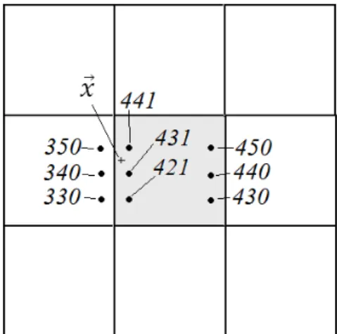
A point of concern is that related to the intersection of the influence domains associated to two neighboring nodes. Take a look at Fig.2.5, and suppose we want to find out at point . The influence domains of the 3 nodes that influence overlap with each other. But in meshless methods, overlapping of influence domains is freely allowed. The 3 nodes in Fig.2.5 act on point , or, equivalently, point belongs to each one of the 3 influence domains that extend until . So, we have another proposition valid in meshless methods:

Proposition 2.2 Influence domains of neighboring nodes can freely overlap, i.e., if and are two nodes, it may occur that

By now, the main feature of meshless approximation should be apparent. If someone wants to calculate at a point , than he first have to find all neighbor nodes that influence . This is a set of nodes hereby represented by . can be structured in such a way that it returns the set of the closest nodes that influence point . Once this set is determined, then we proceed to the application of (2.10). But there are two questions of vital interest here, which seem to have been overrun. The first: What about the values of the nodal parameters ? Equation (2.10) is a weighted sum, but we do not know anything about the weights. How could it be that way? The second: How do we calculate the shape functions ?