A New Polynomial Method for Solving Fredholm –Volterra Integral Equations

A New Polynomial Method for Solving

Fredholm –Volterra Integral Equations

K. Krishnaveni1*, K. Kannan2, S. Raja Balachandar3

Department of Mathematics, School of Humanities and Sciences, SASTRA University, Thanjavur-613401,

Tamilnadu, India. 1

drkveni2012@gmail.com, 2

kkannan@maths.sastra.edu, 3

srbala09@gmail.com

Abstract— A new polynomial method to solve Volterra–Fredholm Integral equations is presented in

this work. The method is based upon ShiftedLegendre Polynomials. The properties of ShiftedLegendre

Polynomials and together with Gaussian integration formula are presented and are utilized to reduce the computation of Volterra–Fredholm Integral equations to a system of algebraic equations. Some numerical examples are selected to illustrate the proposed method also the theoretical analysis of shifted Legendre polynomial method such as convergence and error analysis has been discussed. The results demonstrate reliability and efficiency of the proposed method.

Keyword- Shifted Legendre Polynomials; Nonlinear Integro-Differential equations; Volterra–Fredholm Integral equations; Approximate Solution; Convergence Analysis.

I. INTRODUCTION

Mathematical modeling of physical phenomena namely fluid dynamics, biological models, chemical kinetics and other disciplines lead to linear / nonlinear integro-differential equations. The various types of linear / nonlinear integro-differential equations particularly Fredholm, Volterra, Volterra–Hammerstein, Fredholm-Volterra, impulse integro-differential equations and singular integro-differential equations with their solution methods are reported in [1-36].

These methods are divided into two category namely analytical methods and numerical methods. The Fourier function [2], Adomian decomposition method [13], Homotopy perturbation method [13,14,18-20,23,24,27] are some of the analytical methods used to solve the integral equations . The theoretical analysis such as convergence and error analysis has been discussed in detailed manner. The numerical methods for solving nonlinear integro-differential are Galerkin technique [8,16,23], piecewise interpolation [9], collocation-type method or iterative method [5-7, 32-35], wavelets [3,4,11,12,29] and other methods [10, 31,36] that provide error analysis for particular problem type.

Recently, Legendre polynomial based methods [37-43]are used to obtain the fast solutions problems of science and engineering. The main characteristic behind in this technique is that it reduces these problems to those of solving a system of linear /nonlinear algebraic equations thus greatly simplifying the problem. In this Legendre polynomial method, a truncated orthogonal series is used for numerical integration of differential equations, with a goal of obtaining efficient computational solutions. Shifted Legendre polynomial method SLPM [44] is the next version of Legendre polynomial with shifting property to shift the interval from [-1, 1] into [0, 1].

The various applications of shifted Legendre polynomials had been studied by many researchers and several papers [44-48] have appeared in the literature, concerned with operational matrix based techniques. Theoretical analyses such as error analysis and convergence have also been discussed to demonstrate its potential use. In this paper , we intend to extend the application of SLPM to find the approximate solution of a nonlinear Fredholm–Volterra integral equation[38]

dt t y F t x K x

f x y

x

)) ( ( ) , ( )

( ) (

0 1 1



+

=

λ

( , ) ( ( )) , 0 , 1,

1

0 2

2 ≤ ≤

+

λ



K x t G y t dt x t (1)

where f (x), the kernels K1(x, t) and K2(x, t) are assumed to be in L2(R) on the interval 0 ≤ x, t ≤ 1, which is the general form of [49,50].

The method consists of expanding the solution by shifted Legendre polynomial with unknown coefficients. The properties of shifted Legendre polynomial together with the Gaussian integration formula [30] are then utilized to evaluate the unknown coefficients and we find an approximate solution to Eq. (1).

and 5 provide the convergence and error analysis of SLPM. In Section 6, we demonstrate the accuracy of the proposed scheme by considering numerical examples. The salient features of SLPM and concluding remarks are discussed in Section 7 and 8 respectively.

II. SHIFTEDLEGENDREPOLYNOMIALSANDITSPROPERTIES In this section, we discuss Legendre polynomials and its function approximation[37-43]. A. Legendre polynomials

The Legendre polynomials are defined on the interval [-1, 1] and can be determined with the aid of the following recurrence formulae:

,...,

2

,

1

),

(

1

)

(

1

1

2

)

(

₁ 1

=

+

−

+

+

=

₋

+

L

z

i

i

i

z

zL

i

i

z

L

_{i i i} where

L

₀

(

z

)

=

1

and

L

₁

(

z

)

=

z

.

B. Shifted Legendre polynomials

In order to use these polynomials on the interval

x

∈

[

0

,

1

]

, recently Saadatmandi [44] utilized the so-called shifted Legendre polynomials by introducing the change of variable

z

=

2

x

−

1

.

Let the shifted Legendre polynomials

L

_i

(

2

x

−

1

)

be denoted by

P

_i

(

x

)

. Then

P

_i

(

x

)

can be obtained as follows:

,...,

2

,

1

),

(

1

)

(

)

1

(

)

1

2

)(

1

2

(

)

(

₁ 1

=

+

−

+

−

+

=

−

+

P

x

i

i

i

x

P

i

x

i

x

P

_{i i i} (2)

where

P

₀

(

x

)

=

1

and

P

₁

(

x

)

=

2

x

−

1

.

The analytic form of the shifted Legendre polynomial

P

_i

(

x

)

of degree i given by

2

0

(

)!

(

!

)

)!

(

)

1

(

)

(

k

x

k

i

k

i

x

P

k i k k i i



= +

−

+

−

=

. (3)

Note that

P

_i

(

0

)

=

(

−

1

)

iand

P

_i

(

1

)

=

1

.

The orthogonality condition is











≠

=

+

=

1

0

0

.

,

1

2

1

)

(

)

(

j

i

for

j

i

for

i

dx

x

P

x

P

_{i j} (4)

A function y(x), square integrable in [0,1], may be expressed in terms of shifted Legendre polynomials as



∞ =

=

0

)

(

)

(

j j j

P

x

c

x

y

,

where the coefficients

c

_jare given by

(

2

1

)

(

)

(

)

,

1

,

2

,....

1

0

=

+

=

j



y

x

P

x

dx

j

c

_{j j}

C. Function approximation

In practice, only the first (m+1) terms of shifted Legendre polynomials are considered. Then we have

),

(

)

(

)

(

0

x

C

x

P

c

x

y

T m j j

j

=

Φ

=



=

(5)

where the shifted Legendre coefficient vector C and the shifted Legendre vector

Φ

(

x

)

are given by

],

,...,

[

_{0 m}

T

c

c

C

=

.

)]

(

),...,

(

),

(

[

)

(

x

=

P

₀

x

P

₁

x

p

_m

x

T

Φ

(6) III.SOLUTION OF THE NONLINEAR VOLTERRA–FREDHOLM INTEGRAL EQUATIONS

Consider the nonlinear Volterra–Fredholm integral equations given in Eq. (1). In order to use Legendre polynomials, we first approximate y(x) as

)

(

)

(

x

C

x

dt

t

C

F

t

x

K

x

f

x

C

T x T

))

(

(

)

,

(

)

(

)

(

0 1 1

Φ

+

=

Φ

λ



K

(

x

,

t

)

G

(

C

T

(

t

))

dt

1

0 2

2

Φ

+

λ



(8)

We now collocate Eq.(8) at m+1 points xi as

dt

t

C

F

t

x

K

x

f

x

C

T x i i i T i

))

(

(

)

,

(

)

(

)

(

0 1 1

Φ

+

=

Φ

λ



_K

_x

_t

_G

_C

T

_t

_dt

i

,

)

(

(

))

(

1

0 2

2

Φ

+

λ



(9)

Suitable collocation points are zeros of Chebyshev polynomials [30]

(

)

1

1

,

1

1

2

cos



=

+











+

+

=

i

to

m

m

i

x

_i

π

.

In order to use the Gaussian integration formula for Eq. (9), we transfer the t-intervals [0,xi] and [0, 1] into τ1 and τ2 intervals [−1, 1] by means of the transformations

,

1

2

,

1

2

2

1

=

t

−

=

t

−

x

_i

τ

τ

Let

H

1

(

x

,

t

)

K

1

(

x

,

t

)

F

(

C

(

t

))

,

T i

i

=

Φ

H

₂

(

x

i

,

t

)

=

K

₂

(

x

i

,

t

)

G

(

C

T

Φ

(

t

))

Eq. (9) may then be restated as

2 1 1 2 2 2 1 1 1 1 1

1 ( 1)

2 1 , 2 ) 1 ( 2 , 2 ) ( )

(x f x

λ

x H x x

τ

d

τ

λ

H x

τ

d

τ

C i _i

i i i i T





− −       ₊ +       ₊ + =

Φ By using the Gaussian integration formula we get

      ₊ +       ₊ + ≈

Φ





= = ) 1 ( 2 1 , 2 ) 1 ( 2 , 2 ) ( )

( 2 2

1 2 2 1 1 1 1 1 2 1 j i s j j j i i s j j i i i T x H x x H x x f x

C λ ω τ λ ω τ i= 1 to M+1, (10)

where τ1j and τ2j are s1 and s2 zeros of Legendre polynomials

P

s₁+₁ and

P

s2+2respectively , and w1j , w2j are the

corresponding weights given in [12].

The idea behind the above approximation is the exactness of the Gaussian integration formula for polynomials of degree not exceeding ₁

1

2

_{s +} and ₂

2

2

_{s +} . Eq. (10) gives M+1 nonlinear algebraic equation which can be

solved for the elements of

C

T in Eq. (7) using Newton’s iterative method.

IV. CONVERGENCE ANALYSIS

Theorem 4.1: Convergence theorem

The series solution Eq.( 5) of Eq. (1) using SLPM converges towards y(x).

Proof:

Let L2(R) be the Hilbert space and ₂

0

(

)!

(

!

)

)!

(

)

1

(

)

(

k

x

k

i

k

i

x

P

k i k k i i



= +

−

+

−

=

Let

( )



( )

=

=

m

j j j

P

x

c

x

y

0

where

=

(

+

) ( ) ( )



1

0

1

2

j

y

x

P

x

dx

c

_{j j}

c

_j

=

(

2

j

+

1

) ( ) ( )

y

x

,

P

_j

x

where

.

,

.

represents an inner product.

( ) (

)



( ) ( )

( )

=

+

=

n i j j

x

P

x

P

x

y

j

x

y

1

,

1

2

where j=1,2,3, …

Define the sequence of partial sums {Sn} of

(

α

j

P

j

( )

x

)

; let Sn and Sm be arbitrary partial sums with

n

≥

m

.

We are going to prove that {Sn} is a Cauchy sequence in Hilbert space.

Let



( )

=

=

n j j j

n

P

x

S

1

α

( )

(

) ( )



( )

−

+

=

n j j j

n

j

y

x

P

x

S

x

y

1

,

1

2

,

α

=

(

)



( ) ( )

=

+

n j j

j

y

x

P

x

j

1

,

1

2

α

=

(

)



−

+

n j j j

j

1

1

2

α

α

=

(

)



−

+

n j j

j

1 2

1

2

α

We will claim that

1 2 2 1 2 + = −



+ = j S S j n m j m n α

for n > m.

(ie)

( )

2 1 2



+ =

=

−

n m j j j m

n

S

P

x

S

α

( )



( )



+ = + =

=

n m j j j n m i i

i

P

x

P

x

1 1

,

α

α

=

 

( ) ( )

+ = = + n m i j i j n m j

i P x P x 1 1 , α α =

_











+



+

=

2

1

1

1

j

j n m j j

α

α

=



+ =

+

n m j j

j

1 2

1

2

α

i.e



+ =

+

=

−

n m j j m n

j

S

S

1 2 2

1

2

α

for n > m.

From Bessel’s inequality, we have



∞

=1 2

j j

α

is convergent and hence

2 m

n

S

S

−

→

0

as

m

,

n

→

∞

.

i.e

S

n

−

S

m

→

0

and {Sn} is a Cauchy sequence and it converges to say ‘s’.

We assert that y(x) = s

Infact,

s

−

y

( ) ( )

x

,

P

j

x

=

s

,

P

j

( )

x

−

y

( ) ( )

x

,

P

j

x

= _{n j}

( )

_j

n

x

P

S

Lt

−

α

∞ →

,

= _{n j}

( )

_j

n

x

P

S

Lt

−

α

∞ →

,

=

α

j

−

α

j

Hence

y

( )

x

=

s

and



( )

= m

j j j

P

x

C

0

converges to y(x) and this completes the proof. As the convergence has been

proved, consistency and stability are ensured automatically.

V. ERROR ANALYSIS

In this part, an error estimation for the approximate solution of Eq.(1) is discussed. Let us consider

( )

x

y

( )

x

y

( )

x

e

_n

=

−

as the error function of the approximate solution

y

( )

x

for

y

( )

x

, where

y

( )

x

is the exact solution of Eq.(1).



∞

=

=

0

)

(

)

(

j

j j

P

x

c

x

y

(11)

and

(

)

(

)

(

)

0

x

C

x

P

c

x

y

T

m

j

j

j

=

Φ

=



=

( )

x

C

x

H

( )

x

y

=

T

Φ

(

)

+

_n where

H

_n

( )

x

is the perturbation term.

( )

x

y

( )

x

C

(

x

)

H

_n

=

−

T

Φ

. (12) We proceed to find an approximation

e

_n

( )

x

to the error function

e

_n

( )

x

in the same way as we did before for

the solution of the problem. Subtracting Eq. (12) from Eq. (11), the error function

e

_n

( )

t

satisfies the problem.

( )

x

C

x

( )

x

e

n

−

T

Φ

(

)

=

−

H

n (13)

It should be noted that in order to construct the approximate

e

n

( )

x

to

e

n

( )

x

, only Eq. (13) needs to be

recalculated in the same way as we did before for the solution of Eq.(11).

VI. IIUSTRATIVEEXAMPLES In this section, we examine the performance of SLPM with some examples.

Example 1

Consider the nonlinear Volterra–Fredholm integral equation given in [38] by

,

4

5

3

5

3

1

30

1

)

(

₌

₋

6

₊

4

₋

2

₊

₋

x

x

x

x

x

y

(

x

t

)

[

y

t

]

dt

(

x

t

)

[

y

t

]

dt

x

)

(

)

(

0

1

0 2



−

+



+

+

.

1

,

0

≤

x

t

≤

(14)

We apply the method presented in this paper and solve Eq.(14) with m=3 we get the following algebraic equations

(1/2)c0 – (7/6)c1 + c2-c3=-(5/4) -c0+2c1 – 6c2+12c3=(5/3)

(1/2)c02+(1/2) c12+(1/2)c22+(1/2)c32 –c0c1+c0c2-c0c3-c1c2+c1c3-c2c3-6c2+30c3=1 (-2/3)c12-2c22-4c32+(2/3)c0c1-2c0c2+4c0c3+(8/3)c1c2-(14/3)c1c3+6c2c3-20c3=0 From these equations we find c0 = -1.6667, c1 = 0.5,c2 =0.1667, c3 =0 and y(x)=c0

p

₀ +c1

p

1+c2

p

2+c3

p

3= x

2

-2, which is the exact solution.

Example 2

Consider the nonlinear Volterra integral equation given in [38] by

[

(

)

]

,

3

1

)

3

exp(

3

1

)

exp(

)

(

3

0

dt

t

y

x

x

x

y

x



+

+

−

=

(15)

We apply the method presented in this paper and solve Eq.(15) with m=2 we get the following algebraic equations;

c0 – c1 +c2=1

18c0c22+24c0c1c2 -6c2=1

From these equations we find c0 = 1.6667, c1 = 0.75, c2 =0.0833 and y(x) =

2

1

2

x

x

+

+

The closed solution of y(x) =

e

x which is the exact solution for larger values of m. TABLE 1 shows the error for example 2 for different values of m with exact solution.

TABLE 1

The errors for Example 2 at m=4,10,15

m _{X Exact SLPM Error}

4 _{0 1 1 0}

0.2 1.221403 1.2213 0.0001027

0.4 1.491825 1.4907 0.0011246 0.6 1.822119 1.816 0.0061188 0.8 2.225541 2.2053 0.0202409 1 2.718282 2.6667 0.0512818

10 _{0 1 1 0}

0.2 1.221403 1.2214 0.0000027 0.4 1.491825 1.4918 0.0000246

0.6 1.822119 1.8221 0.0000188 0.8 2.225541 2.2255 0.0000409 1 2.718282 2.7183 -0.0000182

15 _{0 1 1 0}

0.2 1.221403 1.2214 0.0000027 0.4 1.491825 1.4918 0.0000246 0.6 1.822119 1.8221 0.0000188 0.8 2.225541 2.2255 0.0000409 1 2.718282 2.7183 -0.0000182

Example 3

Consider the Integro-differential equation[51]

1

3

4

)

(

)

(

)

(

'

1

0

+

−

+

=



x

sy

s

ds

y

x

x

x

y

; y(0)=0 (16)

We apply the method presented in this paper and solve Eq.(16) with m=3

(ie)



=

=

3

0

)

(

)

(

j

j j

P

x

c

x

y

we get the following algebraic equations

c0 – 3c1 + 7c2-13 c3=-1

(1/2) c0 + (13/6)c1 – 18c2+72 c3=(4/3) 6c2-90c3=0

and from the initial condition y(0)=0, we have c0 - c1 + c2 -c3=0 From these equations we find c0 = 0.5, c1 = 0.5, c2 = 0, c3 = 0.

Using Eq. (6) we get y(x)=c0

p

0 +c1

p

1+c2

p

2+c3

p

3= x, which is the exact solution. Example 4

x

e

x

y

ds

s

y

x

x

y

=



+

+

x

−

1

0

)

(

)

(

)

(

'

y(0)=0 (17)

We apply the method presented in this paper and solve Eq.(17) with m=3 we get the following algebraic equations

c0 - c1 + c2- c3=0 c0 – 3c1 +7c2-13c3=-1 c0 +2c1 -18c2+72c3=0 6 c2 -90c3=-(1/2)

From these equations we find c0 = 0.9474, c1 = 1.2079, c2 = 0.2851, c3 = 0.0246.

The closed solution of y(x) =

xe

x which is the exact solution for larger values of m. . TABLE 2 shows the error for example 2 for different values of m with exact solution.

TABLE 2

The errors for Example 4 at m=4,10,15

m _{X Exact SLPM Error}

4 _{0 0 0 0}

0.2 0.244281 0.244 2.81E-04

0.4 0.59673 0.592 4.73E-04

0.6 1.093271 1.068 0.02527

0.8 1.780433 1.696 0.08443

1 2.718282 2.5 0.21828

10 _{0 0 0 0}

0.2 0.244281 0.2443 -2E-05

0.4 0.59673 0.5967 3.00E-10

0.6 1.093271 1.0933 1.77E-08 0.8 1.780433 1.7804 3.21E-07 1 2.718282 2.7183 -1.8E-05

15 _{0 0 0 0}

0.2 0.244281 0.2443 -2E-05

0.4 0.59673 0.5967 2.98E-05 0.6 1.093271 1.0933 -2.9E-05 0.8 1.780433 1.7804 3.27E-05

1 2.718282 2.7183 -1.2E-05

Example 5

Consider the Integro-differential equation[51]



−

+

=

x

dt

t

y

x

t

x

x

y

0

)

(

)

(

)

(

(18)

We apply the method presented in this paper and solve Eq.(18) with m=3 we get the following algebraic equations

c0 - c1 + c2-c3=0 2c1 – 6c2+12 c3=1

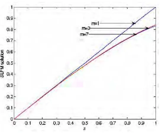
From these equations we find c0 = 0.4583, c1 = 0.4250, c2 =-0.0417, c3 =-0.0083.and y(x) =

6

3

x

x

−

. The closed solution of y(x) = sin x, which is the exact solution for larger values of m and it has been depicted

in Fig 1.

Fig 1: SLPM solution of Example 5 for different values of m

Example 6

Consider the nonlinear boundary value problem for the integro-differential equations related to the Blasius problem [49].

0

,

)

(

''

)

(

2

1

)

(

''

0

<

<

∞

−

−

=



y

t

y

t

dt

x

x

y

x

α

(19)

subject to the boundary conditions

y

( )

0

=

1

,

y

'

( )

0

=

1

andy'(x)=0when x→−∞

We solve (19) with m=6.

y(x)=c0

p

0+c1

p

1+c2

p

2+c3

p

3

= 2 4 2 5

240

1

48

1

2

1

x

x

x

x

+

α

−

α

−

α

+… which is the exact solution reported in [49] VII. SALIENTFEATURES

The proposed method is very simple in application and SLPM the solution can be obtained in bigger interval. Unlike Adomian Decomposition Method(ADM), Homotopy Analysis Method(HAM) and Homotopy Perturbation Method(HPM), the SLPM do not require the Adomian polynomials, Lagrange multiplier, correction functional, stationary conditions and calculating integrals, which eliminate the complications that exists in the ADM, HAM and MHPM.

VIII. CONCLUSION

In this work, we have proposed the shifted Legendre polynomials method (SLPM) for Solution of thelinear and nonlinear Volterra-Fredholm integral equations. The properties of shifted Legendre polynomials are used to reduce the problem to the solution of algebraic equations with appropriate coefficients which provide exact solutions for all the chosen problems. Moreover, the convergence analysis, error estimations clearly reveal its validity and potential use of applicability to any phenomena governed by this equation. In future, we may use this proposed method for solving other non linear fractional integro-differential equations and fractional partial differential equations also.

ACKNOWLEDGMENT

The authors wish to express their gratitude to the referees for their careful reading of the manuscript and helpful suggestions.

REFERENCES

[1] Brunmer, H.: Collocation method for volterra integral and related function equation, Cambridge Monograph on Applied and Computational Mathematics, Cambridge University Press, Cambridge MA (2004).

[2] B.Asady, M.Tavassoli Kajani, A.Hadi Vencheh, A.Heydari, Solving second kind integral equations with hybrid Fourier and block- pulse functions, Appl.math.Comput.160, 2005,517-522.

[3] I.Daubechies, Ten Lectures on wavelets, SIAM, Philadelphia, PA ,1992.

[4] W.Fang, Y.Wang, Y.Xu, An implementation of fast wavelet Galerkin methods for integral equations of the second kind,

J.Sci.comput.20, 2004,277-302.

[5] S. Kumar, I.H. Sloan, A new collocation-type method for Hammerstein integral equations, J. Math. Comput.48, 1987,123–129. [6] H. Brunner, Implicitly linear collocation method for nonlinear Volterra equations, J.Appl. Num. Math.9,1992,235–247.

[7] H. Guoqiang, Asymptotic error expansion variation of a collocation method for Volterra–Hammerstein equations, J. Appl. Num. Math. 13, 1993,357–369.

[8] E. Babolian and L. M. Delves, An augmented Galerkin method for first kind Fredholm equations, Journal of the Institute of Mathematics and Its Applications, 24(2), 1979,157–174.

[9] G. Hanna, J. Roumeliotis, and A. Kucera, Collocation and Fredholm integral equations of the first kind, Journal of Inequalities in Pure and Applied Mathematics,6(5), 2005,article 131,1–8.

[10] B. A. Lewis, On the numerical solution of Fredholm integral equations of the first kind, Journal of the Institute of Mathematics and Its Applications, 1975;16(2): 207–220.

[11] K. Maleknejad, R. Mollapourasl, and K. Nouri, Convergence of numerical solution of the Fredholm integral equation of the first kind with degenerate kernel, Applied Mathematics and Computation,181(2), 2006,1000–1007.

[12] X. Shang and D. Han, Numerical solution of Fredholm integral equations of the first kind by using linear Legendre multi-wavelets,

Applied Mathematics and Computation,191(2),2007,440–444.

[13] S. Abbasbandy, Numerical solutions of the integral equations: homotopy perturbation method and Adomian’s decomposition method,

Appl. Math. Comput.173(2–3), 2006,493–500.

[14] S. Abbasbandy, Application of He’s homotopy perturbation method to functional integral equations, Chaos Soliton. Fract.,31(5), 2007,1243–1247.

[15] R.P. Agarwal, Boundary value problems for higher order integro-differential equations, Nonlinear Analysis, Theory, Meth. Appl. 7(3), 1983,259-270.

[16] A. Avudainayagam, C. Vani, Wavelet-Galerkin method for integro-differential equations, Appl. Numer. Math.32, 2000,247–254. [17] Elcin Yusufoglu (Agadjanov), Numerical solving initial value problem for Fredholm type linear integro-differential equation system,

Journal of the Franklin Institute 346,2009,636–649.

[18] M. El-Shahed, Application of He’s homotopy perturbation method to Volterra’s integro-differential equation, Int. J. Nonlinear Sci. Numer. Simul.6(2),2005,163– 168.

[19] M. Ghasemi ,M. Tavassoli kajani C, and E. Babolian, Application of He’s homotopy perturbation method to nonlinear integro- differential equations, Appl. Math.Comput.188, 2007,538–548.

[20] M. Ghasemi ,M. Tavassoli kajani C, and E. Babolian, Comparison between wavelet Galerkin method and homotopy perturbation method for the nonlinear integro-differential equations, Computers and Mathematics with Applications 54,2007,1162–1168. [21] M. Ghasemi ,M. Tavassoli kajani C, and E. Babolian ,Numerical solution of linear integro-differential equations by using sine-cosine

wavelet method, Applied Mathematics and Computation180, 2006,569–574.

[22] M. Ghasemi ,M. Tavassoli kajani C, and E. Babolian, Comparison between the homotopy perturbation method and the sine–cosine wavelet method for solving linear integro-differential equations, Computers and Mathematics with Applications 54,2007,1162–1168. [23] M. Ghasemi ,M. Tavassoli kajani C, and E. Babolian, Numerical solutions of the nonlinear integro-differential equations: Wavelet-

Galerkin method and homotopy perturbation method, Appl. Math. Comput.188, 2007,450–455.

[24] Jichao Zhao, Robert M. Corless, Compact finite difference method for integro- differential equations, Appl. Math. Comput 177, 2006,271–288.

[25] J. Morchalo, On two point boundary value problem for integro-differential equation of second order, Fasc. Math.9, 1975,51-56. [26] J. Morchalo, On two point boundary value problem for integro-differential equation of higher order, Fasc. Math.9,1975,77-96. [27] S.R.Seyed Alizadeh, G.G. Domairry, and S. Karimpour, An Approximation of the Analytical Solution of the Linear and

Nonlinear Integro-Differential Equations by Homotopy Perturbation Method, Acta Appl Math 104, 2008, 355–366.

[28] S.Shahmorad, Numerical solution of the general form linear Fredholm-Volterra integro-differential equations by Tau method with an error estimation, Appl. Math. Comput, 167, 2005,1418-1429.

[29] Ulo Lepik , Haar wavelet method for nonlinear integro-differential equations, Appl. Math. Comput.176, 2006,324–333. [30] A. Constantinides, Applied Numerical Methods with Personal Computers, McGraw- Hill, New York, 1987.

[31] Zhang Lingling, Yin Jingyi, Liu Junguo, The Solutions of Initial Value Problems for Nonlinear Fourth-Order Impulsive Integro- Differential Equations in Banach Spaces, WSEAS TRANS -ACTIONS on MATHEMATICS, 3(11) 2012, 204-221.

[32] Iurie Caraus, Nikos E. Mastoraskis, The Numerical Solution for Singular Integro- Differential Equation in Generalized Holder Spaces, WSEAS TRANSACTIONS on MATHEMATICS, 5( 5) 2006, 439- 444.

TRANSACTIONS on MATHEMATICS. 6(11), 2007, 859-864.

[34] Iurie Caraus, Nikos E. Mastoraskis, Convergence of the Collocation Methods for Singular Integro- Differential Equations in Lebesgue Spaces, WSEAS TRANSACTIONS on MATHEMATICS, Issue Volume 6,November 2007 ISSN: 1109-2769.

[35] Iurie Caraus, Nikos E. Mastorakis, The stability of collocation methods for approximate solution of singular integro- differential equations. WSEAS TRANSACTIONS on MATHEMATICS, 4(7), 2008, 121-129.

[36] Feras M. Al Faqih, Nikos E. Mastorakis, Iurie Caraus, Approximate Solution of Systems of Singular Integro- Differential Equations by Reduction Method in Generalized Holder spaces WSEAS TRANSACTIONS on MATHEMATICS, 7(11), 2012, 625-633. [37] M.Razzagi, S.Yousefi, Legendre wavelets method for the solution of nonlinear problems in the calculus of variations, Math.

Comput. Modell. , 34 ;2001; 45-54.

[38] S.Yousefi, M.Razzaghi, Legendre wavelets method for the nonlinear Volterra-Fredholm integral equations, Math. Comput. Simul, 70;2005; 1-8.

[39] S.A.Yousefi, Legendre scaling function for solving generalized Emden-Fowler equation, Int. J. Inf. Sys. Sci. , 3;2007; 243-250. [40] S.A.Yousefi , Legendre wavelets method for solving differential equations of Lane-emden type, Appl. Math. Comput.,181; 2006;

1417-1422.

[41] S.G.Venkatesh, S.K.Ayyaswamy, S.Raja Balachandar, The Legendre wavelet method for solving initial value problems of Bratu- type, Comput. Math. Appl., 63;2012;1287–1295.

[42] S.G.Venkatesh, S.K.Ayyaswamy, S.Raja Balachandar, Convergence Analysis of Legendre wavelets method for solving Fredholm Integral equations, Appl. Math. Sci., 6; 2012;2289-2296.

[43] S.G.Venkatesh, S.K.Ayyaswamy, S.Raja Balachandar, Legendre approximation solution for a class of higher-order Volterra integro- differential equations, Ain Shams Eng J 2012;3:417–22..

[44] A.Saadatmandi, M.Dehghan., A new operational matrix matrix for solving fractional-order differential equations, Computers and Mathematics with Applications,59, 2010,1326-1336.

[45] A. Saadatmandi, M. Razzaghi, M. Dehghan, Hartley series approximations for the parabolic equations, Intern. J. Comput. Math. 82, 2005,1149-1156.

[46] A. Saadatmandi, M. Dehghan, A Tau method for the one-dimensional parabolic inverse problem subject to temperature overspecification, Comput.Math. Appl. 52, 2006,933-940.

[47] A. Saadatmandi, M. Dehghan, Numerical solution of the one-dimensional wave equation with an integral condition, Numer. Methods Partial Differential Equations 23, 2007,282-292.

[48] A. Saadatmandi, M. Dehghan, Numerical solution of a mathematical model for capillary formation in tumor angiogenesis via the tau method, Commun.Numer. Methods. Eng.24, 2008,467-1474.

[49] A.M.Wazwaz ,A reliable algorithm for solving boundary value problems for higher-order integro-differential equations, Appl. Math. Comput 118, 2001,327- 342.

[50] S. Yalcinbas, Taylor polynomial solution of nonlinear Volterra–Fredholm integral equations, Appl. Math. Comput. 127, 2002,,195–206.