ISSN 0101-8205 www.scielo.br/cam
On the convergence of derivatives of B-splines
to derivatives of the Gaussian function
RALPH BRINKS
Philips Research Laboratories, Weisshausstrasse 2, 52066 Aachen, Germany E-mail: [email protected]
Abstract. In 1992 Unser and colleagues proved that the sequence of normalized and scaled
B-splines Bm tends to the Gaussian function as the ordermincreases, [1]. In this article the result of Unser et al. is extended to the derivatives of the B-splines. As a consequence, a certain sequence of wavelets defined by B-splines, tends to the famous Mexican hat wavelet. Another consequence can be observed in the continuous wavelet transform (CWT) of a function analyzed with different B-spline wavelets.
Mathematical subject classification: 43A15, 42C40, 65T60, 65R10.
Key words: B-splines, Gaussian function, Continuous wavelet transform, Mexican hat wavelet,
Scalogram.
1 Introduction
In 1992 Unser and colleagues proved that the sequence of normalized and scaled B-splinesBmtends to the Gaussian function as the ordermincreases, [1]. In this article the result of Unser et al. is extended to the derivatives of the B-splines. After some definitions and introductions this is done in the second section.
Due to numerical reasons it has become common to use B-splines as analyzing functions (wavelets) in wavelet analysis. Two implications of the convergence result of the second section in wavelet analysis are presented in the third sec-tion. First, a certain sequence of wavelets defined by B-splines tends to the
famous Mexican hat wavelet. Second, similarities in continuous wavelet trans-form (CWT) can be observed, when a function is analyzed with different B-spline wavelets.
2 B-splines: definition and some properties
Let p∈R≥1andLp(R)as usual denote the set Lp(R)=
f :R→C| f measurable,
∞
−∞
|f(t)|pdt<∞
.
For p=2 and f,g∈ L2(R)define the inner product
f,g :=
∞
−∞
f(t)g(t)dt
and the norm
f :=f, f,
makingL2(R)to a Hilbert space. For f,g ∈L2(R)the function f∗gis defined as
(f ∗g)(t):=
∞
−∞
f(t−y)g(y)dy.
f ∗gis called convolution product of f andgand is inL2(R).
For f ∈ L1(R)define the Fourier transform f∧and the inverse Fourier
trans-form f∨as
f∧(ω):=
∞
−∞
f(t)e−iωtdt,
f∨(ω):= 1
2π
∞
−∞
f(t)eiωtdt.
This definition can be extended to functions f ∈ L2(R), see for example [2]. Now let us define the cardinal B-splines:
Definition 2.1. Define
B0(t):=
and let Bmbe defined as
Bm := B0∗Bm−1, m ∈N. ThenBm, m ∈N0,has the compact support
−m+21, m+1
2
and is inCm−1(R), (C−1(R)denotes the set of the piecewise constant functions). The Bm are the famouscardinal B-Splines.
B-splines play an important role in computer-aided design (CAD) and signal processing. For an extensive monography see [3].
For allBm, m∈N0, it holdsBm ∈ L1(R)
∩L2(R)and Bm∧(ω)=sinc(m+1)(ω/2), where sinc denotes thesinus cardinalisfunction:
sinc(t):=
sin(t)
t , fort =0; 1, fort =0.
After the necessary definitions have been provided, we can come to the main result of this article. Unser and colleagues in [1] have shown that normalized and scaled versions of the B-splines tend to the Gaussian function:
lim m→∞
m+1 12 Bm
m+1 12 ·x
= √1
2π exp
−x 2 2 , (2.1)
where the limit may be taken pointwise or in Lp(R), p ∈ [2,∞).
Now it is shown that taking thek-th derivative of both sides of equation (2.1) is possible. It holds:
Theorem 2.2. Let be k ∈ N0 then form ≥ k +1 the sequence of the k-th
derivativesB(k)
m of the cardinal B-splines converges to thek-th derivative of the
Gaussian function, lim m→∞
m+1 12
k+21
Bm(k)
m+1 12 ·x
= √1
2π
dkexp −x22
dxk ,
where the limit may be taken pointwise or inLp(R), p∈ [2,∞).
Lemma 2.3. Let bek ∈ N0 and A : R → Rbe a two times continuously
differentiable function with a positive maximum atx0such that
1. A(x0) >0,
2. A′(x0)=0,
3. A′′(x0)= −α2A(x0) <0, α=0,
then for the sequence
An(x)=
1 A(x0)A
x
α +x0
n
=[A1(x)]n
it holds
lim n→∞
xk An
x
√
n
=xkexp
−x 2 2 ,
where the limit is taken pointwise.
Proof. First of all let be k = 0. Define Ln(x) := lnAn
x
√
n
. Then with tn:= √x
n it holds
Ln(x)=nln
A1 x √n =
lnA1√x
n
1/n =x
2 ln [A1(tn)]
(tn)2 . Since it holds A1(0) = 1 and A′
1(0) = 0, for the limit n → ∞, and hence tn→0,we may apply l´Hôpital’s rule twice:
lim
n→∞Ln(x) =x
2 lim n→∞
A′1(tn)
2tn A1(tn) =
x2 2 nlim→∞
A′′1(tn)
A1(tn)+tnA′1(tn)
= x
2 2 A
′′
1(0)= − x2
2 .
Lemma 2.4. Fork ∈N0andn∈N, n >k+2,there is a constantck ∈R>0
such that for
Gk(x):=χR\[−1,1](x)
ck
π2x2 +π k
|x|kexp(−x2)
it holds
Gk ∈ Lp(R), ∀ p ∈ [1,∞),
and
πk |x|k·
sinc πx √ n n
≤ Gk(x).
Proof. The fact thatGk(x)∈ Lp(R),p≥1,may be concluded from exp(−x2)
≤ x−2kforxlarge in modulus. Due to the symmetry we may assumex
≥0.For x ∈ [0,1]it holds
sin(πx)≤πx− π 3x3 3! +
π5
5!, and hence sinc(πx)≤1−x2.
1. Letx ∈
0,√n
.
Then it holds
sincn πx √ n ≤
1− x 2 n
n
.
Now we show that
1− x 2 n
n
≤e−x2.
Let
p(x):=ex2
1− x 2 n
n
,
then it holds
p′(x)= −2
n x 3ex2
1−x 2 n
n−1
<0, ∀x ∈ [0,√n),
2. Letx ∈√
n,∞.
Set
ck := max n>k+2
n(k+2)/2
πn−k−2
.
The existence ofck follows from the convergence of the sequence
n(k+2)/2
πn−k−2
n>k+2
.
Then one follows
nk+22 ≤ ckπn−k−2
√
nk+2√nn−k−2 ≤ ckπn−k−2xn−k−2
√
n xπ
n
≤ xk+2ckπk+2. By noting that
sincn
πx
√
n
≤
√n
πx
n
the hypothesis follows.
Proof of Theorem 2.2. Set A(x):= sinc(x/2),then for Athe assumptions of Lemma 2.3 are fulfilled withα = √1
12.The lemma states that xk An
x
√
n
=xksincn
x 2
12 n
tends toxkexp−x22ifn → ∞.Furthermore, it holds Bm∧=sinc(m+1)(·/2), and Bm ∈Cm−1(R). The later yields fork
≤m−1:
Bm(k)∧(ω)=ikωksinc(m+1)ω 2
Consequently, one obtains
m+1 12
k+21
Bm(k)
m+1 12 ·
∧
(ω)
=ikωksinc(m+1)
ω
2
12 m+1
−→ikωkexp
−ω
2 2
form→ ∞
=ikωk
1
√
2π exp
− t
2 2
∧
(ω)
=
dk dtk
1
√
2π exp
−t
2 2
∧
(ω)
(2.2)
where the limit in equation (2.2) follows from Lemma 2.3 and is meant to be taken pointwise. The Lp-convergence, p
≥ 1, follows from Lebesgue’s Dominated Convergence Theorem, using Lemma 2.4. The hypothesis follows from taking the Fourier transform and the fact that forp∈ [1,2]and1/p+1/q=1 the Fourier transform is a bounded operator fromLp(R)toLq(R),see [2, Sect. V.1].
3 Wavelet analysis
In this section two implications of Theorem 2.2 for wavelet analysis are pre-sented briefly. For a more detailed treatment of wavelet analysis, see for example the books of Daubechies [4] or Chui [5].
Definition 3.1. A function ψ ∈ L2(R)\ {0}is called a wavelet, iffψ fulfills
theadmissibility condition
Cψ :=
∞
−∞ ψ∧(ω)
2
|ω| dω <∞ (3.1)
Example 3.2. Here we give two examples of famous wavelets:
1. TheHaar waveletis defined by
ψ =χ[0,1/2)−χ[1/2,1). 2. The second derivative of the Gaussian exp−t22
ψ (t)= d
2 dt2exp
−t
2 2
=(t2−1)exp
−t
2 2
is another standard wavelet, the Mexican hat wavelet. The normalized version is 2
π1/4√3(t 2
−1) exp−t22.
3.1 Convergence to the Mexican hat wavelet
The construction of the Mexican hat wavelet as a derivative of the Gaussian function may be generalized:
Proposition 3.3. Letϕ ∈ Ck(R)
∩L2(R)
\ {0},k ∈ N,withϕ(m)(t)
→0as
|t| →0for allm∈ {0, . . . ,k−1}andϕ(k) ∈ L1(R)∩L2(R),then
ψ:= ϕ
(k)
ϕ(k)
is a normalized wavelet.
Proof. First of allψ cannot be constant zero, which would imply thatϕ is a polynomial, what contradicts the assumptions. Without loss of generality assume
ϕ(k)
=1.From Fourier analysis it followsψ∧(ω)=(iω)k·ϕ∧(ω)and hence
∞
−∞ ψ∧(ω)
2
|ω| dω =
|ω|≤1|
ω|2k−1ϕ∧(ω) 2 dω +
|ω|>1
ψ∧(ω)
2
|ω| dω≤
ϕ∧
2
+ψ∧
2
.
With a view to numerical calculations wavelets with compact support are mostly preferred. Thus, the derivatives of the cardinal B-splines Bm, which of course have compact support, are nice candidates for wavelets. For those wavelets, we now can state the first consequence from Theorem 2.2:
Corollary 3.4. Form∈N, m ≥3,define the normalized wavelets
ψm :=
Bm′′ m12+1·
B
′′
m
m+1 12 ·
,
then the sequence(ψm)m≥3converges to the normalized Mexican hat wavelet as
mtends to infinity.
3.2 Similarity in the continuous wavelet transform
The second consequence of the convergence result of the previous section relates to the continuous wavelet transform (CWT). The CWT is an integral transform, which correlates a given function f to the dilated and translated versions of waveletψ.
Definition 3.5. Let f, ψ ∈ L2(R),then define Wψ[f] :R×R=0→R
(β, α)→ √1
|α|
∞
−∞
f(t) ψ
t−β α
dt.
(3.2)
Ifψis a wavelet,Wψ[f]is calledcontinuous wavelet transform (CWT) of f.
Remark 3.6. By Cauchy-Schwarz’s inequality Wψ[f] is well-defined and bounded.
In the continuous wavelet transform (3.2) the parameterα ∈R=0is the scale or dilation parameter, and β ∈ Ris the translation parameter, which may be
and hence the smaller the corresponding analyzed frequency. The CWT is max-imal if the frequency of the input signal f matches that of the corresponding wavelet and the phases coincide.
Hence, for an one-dimensional input signal the transform Wψ[f] is a two-dimensional description of the signal with respect to the timeβand the scaleα.
The(β, α)-space is called parameter plane and a plot ofWψ[f](β, α)
2 against the parameter plane is called ascalogram. Since we are using real wavelets only, henceforth a scalogram is a plot ofWψ[f](β, α)
against the parameter plane.
Those are often arranged as contour plots where the brightness of each pixel represents the modulus of the CWT, see Figure 1.
Figure 1 – Scalogram of a function with analyzing waveletB5′′.The abscissa and ordinate ranges areβ ∈ [0,1]and log2α∈ [−8,−3].The gray value of each pixel corresponds
to the modulus of the CWT. Black means zero, the brighter the more modulus.
The comparison of the zero-lines of different B-Spline wavelets shows an astonishing similarity for the same order of differentiation. For example the zero-lines in the CWT for normalized versions of B4′′,B5′′ and B6′′ are just vertically shifted as may be seen in Figure 2.
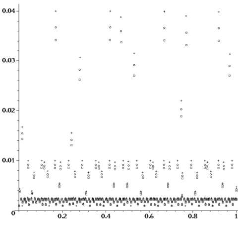
If only the bending points of the zero-lines are plotted in the parameter plane, the shift may be seen more impressively by cascades of three points with the same abscissa values, cf. Figure 3.
Figure 2 – Scalograms for different analyzing wavelets, from top to down: B4′′, B5′′, B6′′, (each normalized). The abscissa and ordinate ranges are β ∈ [0,1] and log2α ∈
[−7,−3].Note the vertical shift.
Figure 3 – Bending points for the same data set but different analyzing wavelets B4′′(+),B5′′(◦),andB6′′().
ψ1.Lets ∈R>0and
ψ2(t)=
√
sψ1(s·t). Then it holds
Wψ2[f](β, α) = 1
√ |α|
∞
−∞
f(t) ψ2
t −β
α
dt
= √s √
|α|
∞
−∞
f(t) ψ1
t −β α/s
dt
= Wψ1[f]
β,α
s
,
which means that for any(β0, α0)∈R×R=0: Wψ2[f](β0, α0)=0⇔Wψ1[f]
β0,
α0 s
=0.
Consequently, each zero (β0, α0) ofWψ2[f] is shifted to the zero
β0,αs0
of Wψ1[f].
Figure 4 – Qualitative similarity ofB4′′,B5′′andB6′′.
Theorem 2.2 explains the vertical shifts of the scalograms by values around 0.9. Form = 4 andm = 5 respectively the ratios of the coefficients inside the arguments m12+1 of Bm′′ and B
′′
m+1 are
√5
/6 ≈ 0.913 and √6/7 ≈ 0.926 respectively.
4 Summary
of the B-splines tends to the Mexican hat wavelet, and second, the CWTs of a function with different B-spline wavelets have astonishing similarities.
REFERENCES
[1] M. Unser, A. Aldroubi and M. Eden,On the Asymptotic Convergence of B-Spline Wavelets to Gabor Functions. IEEE Trans. Inform. Theo.,38(2) (1992).
[2] E.M. Stein and G. Weiss,Introduction to Fourier Analysis on Euclidean Spaces. Princeton University Press, Princeton, 1975.
[3] C. de Boor,A Practical Guide to Splines. Springer-Verlag, New York, 1978.
[4] I. Daubechies,Ten Lectures on Wavelets. SIAM, Philadelphia, 1992.
![Figure 1 – Scalogram of a function with analyzing wavelet B 5 ′′ . The abscissa and ordinate ranges are β ∈ [ 0, 1 ] and log 2 α ∈ [− 8, − 3 ]](https://thumb-eu.123doks.com/thumbv2/123dok_br/18978006.455993/10.892.200.692.489.731/figure-scalogram-function-analyzing-wavelet-abscissa-ordinate-ranges.webp)