Escola de Engenharia
Programa de Pós-Graduação em Engenharia Elétrica
Estabilização Robusta de Sistemas Não Lineares Incertos Utilizando
Representações Algébricas Diferenciais
Sajad Azizi
Tese de Doutorado submetida à Banca Examinadora
designada pelo Colegiado do Programa de
Pós-Graduação em Engenharia Elétrica de Escola de
Enginharia de Universidade Federal de Minas Gerais,
como requisito para obtenção do Título de Doutor em
Engenharia Elétrica.
Orientador: Leonardo Antônio Borges Tôrres
Coorientador: Reinaldo Martinez Palhares
Azizi, Sajad.
A995r Robust stabilization of uncertain nonlinear systems using differential algebraic representations [manuscrito] / Sajad Azizi. - 2017.
89 f., enc.: il.
Orientador: Leonardo Antônio Borges Tôrres. Coorientador: Reinaldo Martinez Palhares.
Tese (doutorado) Universidade Federal de Minas Gerais, Escola de Engenharia.
Bibliografia: f. 78-89.
1. Engenharia elétrica - Teses. 2. Atração de elipsóides - Teses. 3. Representações de álgebras - Teses. 4. Teoria das estruturas - Métodos matriciais - Teses. I. Tôrres, Leonardo Antônio Borges. II. Palhares, Reinaldo Martinez. III. Universidade Federal de Minas Gerais. Escola de Engenharia. IV. Título.
P
HD T
HESISRobust Stabilization of Uncertain Nonlinear
Systems using Differential Algebraic
Representations
Author: Sajad Azizi
Advisers: Leonardo A.B. Torres Reinaldo M. Palhares
Submitted in partial fullfilment of the requirements for the Degree of Doctor of Philosophy at the Federal University of Minas Gerais
Graduate Program in Electrical Engineering
Regional robust stabilization for a class of uncertain MIMO nonlinear systems with parametric
uncertainties is investigated. The closed-loop robust stability is achieved using linear
time-invariant state feedback control. In this context, two cases are investigated: (i) uncertain
nonlin-ear systems resulting from attempts to use the well-known Input-Output Feedback Linnonlin-earization
technique applied considering nominal parameters; and (ii) uncertain nonlinear systems with
input saturation. In both cases, the fact that the uncertain systems have Differential Algebraic
Representations (DAR) is the main theoretical assumption employed to derive sufficient
condi-tions, in the form of Linear Matrix Inequalities (LMI), to solve the corresponding control
prob-lem. The regional character of the stability result obtained using this approach is associated with
the largest ellipsoidal Domain of Attraction (DOA), considered to be inside a given polytopic
region in the closed-loop system state space, which is a byproduct of solving the associated
op-timization problem of searching for appropriate feedback gain matrices. Specifically, the thesis
contributions are new sufficient LMI conditions with new decision variables used to compute the
feedback gain matrices without prior knowledge of an initial stabilizing matrix. The new
con-ditions have also shown favorable comparisons with recently published similar control design
methodologies, particularly for the case of uncertain nonlinear systems with input saturation,
All Praise Is Due to God, Lord of The Worlds. ”Quran 1:2”
I would like to give my sincere thanks and appreciation to my adviser, Prof. Leonardo A. B.
Torres, and my co-adviser, Prof. Reinaldo M. Palhares for all help and support. Also, I would
like to declare my special gratitude to my wife Masoumeh, who has been accompanying me
in any circumstance during my study, and to my dear parents, who have always supported and
encouraged me to progress.
Abstract i
Acknowledgements ii
Contents iii
List of Figures v
List of Tables vii
Abbreviations viii
Notations ix
1 Introduction 1
1.1 Control of Uncertain Nonlinear Dynamical Systems . . . 1
1.2 Motivation. . . 3
1.3 Objectives . . . 7
1.4 Summary of Contributions . . . 8
1.5 Thesis Organization . . . 8
2 Uncertain Nonlinear Dynamical Systems Representations 10 2.1 Linear Parameter Varying Models . . . 11
2.2 Linear Fractional Representations . . . 12
2.3 Differential Algebraic Representations . . . 15
2.4 On the Feedback Linearization of Uncertain Nonlinear Systems . . . 17
2.4.1 Approximate Feedback Linearization . . . 18
2.4.1.1 Approximate Feedback Linearization of Inverted Pendulum . 24 2.4.1.2 Approximate Input/Output Linearization of a MIMO System 26 2.5 On the Representation of Input Saturation . . . 27
2.5.1 Description of Input Saturation. . . 29
3 Stability Analysis of Uncertain Nonlinear Dynamical Systems 33 3.1 Polytopic Descriptions of State Space Regions. . . 33
3.2 Regional Stability and Domain of Attraction . . . 35
3.3 Quadratic Stability and Guaranteed Ellipsoidal DOA . . . 35
3.4 Input-to-State Stability of Internal Dynamics. . . 37
4 State Feedback Control Synthesis for Uncertain Nonlinear Dynamical Systems 39
4.1 Control Synthesis without Input Saturation. . . 39
4.1.1 Control Design . . . 40
4.2 Control Synthesis with Input Saturation . . . 44
4.2.1 Linear Annihilators . . . 44
4.2.2 Control Synthesis for the DAR of Input-saturated Nonlinear System . . 45
5 Numerical Examples 53 5.1 Input/Output Linearizable System with Internal Dynamics . . . 53
5.2 Feedback Linearized Inverted Pendulum without Input Saturation . . . 56
5.3 Lorenz System . . . 59
5.4 SISO System with Input Saturation . . . 63
5.5 MIMO System with Input Saturation . . . 65
5.6 Feedback Linearized Pendulum with Input Saturation . . . 67
6 Final Remarks 72 6.1 Overview . . . 72
6.2 Uncertain Nonlinear Systems Representations . . . 73
6.3 Stability Analysis . . . 74
6.4 State Feedback Control Synthesis . . . 74
6.5 Possible Future Work . . . 74
6.5.1 Reducing Conservatism . . . 74
6.5.2 Study of Non-minimum Phase Systems . . . 75
6.5.3 Inverse Dynamics in The Context of Model Predictive Control . . . 75
6.5.4 Inverse Dynamics in The Context of Passivity Theory. . . 76
1.1 Stability regionΩin a compact regionXin the state space. . . 2
1.2 Different approaches to recast the system. . . 3
1.3 Inverse Dynamics based Control as a feedback linearization strategy. . . 4
1.4 Saturation of input signal and linear state feedback control command. . . 6
2.1 Block diagram of linear parameter varying model (2.1). . . 11
2.2 Linear Fractional Representation of rational system (2.4). . . 13
2.3 Representation of I/O linearized model to DAR model. . . 22
2.4 Schematic of the inverted pendulum dynamics . . . 24
2.5 Input-saturated uncertain nonlinear system. . . 28
2.6 Dead-zone nonlinearity and sector bound condition. . . 29
2.7 Representation of saturated input by the convex combination of linear vectors. . 32
4.1 Differential Algebraic Representation of feedback linearized closed-loop system. 43 5.1 Estimated projected DOA in thez1−z2plane (upper plot) and output trajectories together with the time responses of internal dynamics (lower plot). . . 55
5.2 Output trajectories and time responses of internal dynamics forδ1 = 1.1. . . . 55
5.3 Estimated ellipsoidal DOA and Phase Trajectories of States with Different Bounds ofδ1andδ2. . . 59
5.4 variation of DOA volume versus uncertainty|δ1|growth. . . 60
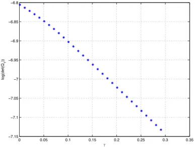
5.5 Variation of the largest guaranteed ellipsoidal DOA volume for different values ofγ. . . 61
5.6 Guaranteed DOA for the Lorenz system together with some state trajectories. . 62
5.7 The variation of largest guaranteed ellipsoidal DOA volume for different values ofγ. . . 64
5.8 DOA and states trajectories for system (5.5). . . 64
5.9 Variation of the largest guaranteed ellipsoidal DOA volume for different values ofγ. . . 65
5.10 Guaranteed ellipsoidal DOA with the system trajectories. . . 66
5.11 Variation of DOA volume versus the growth of uncertainty bound. . . 67
5.12 Guaranteed ellipsoidal DOA with the system trajectories in the presence of un-certainty.. . . 67
5.13 Variation of the largest guaranteed ellipsoidal DOA volume for different values ofγ. . . 69
5.14 Estimated DOA and states trajectories of the inverted pendulum with different bounds ofδ1andδ2.. . . 70
5.15 States trajectories of the inverted pendulum and DOA for |δ1| ≥ 0.137 and different bounds ofδ2. . . 70
6.1 Inverse Dynamics based Control in the context of nonlinear model predictive
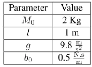
5.1 Parameters of Inverted Pendulum . . . 58
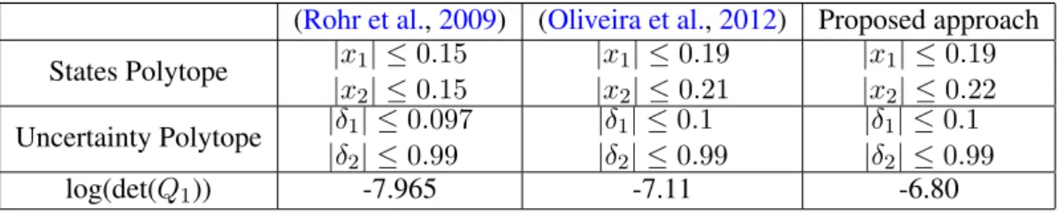
5.2 Comparison of Results of DOA for Inverted Pendulum . . . 59
5.3 Characteristics of DOA of system (5.4). . . 64
5.4 Characteristics of state space polytope of system (5.6). . . 66
5.5 Characteristics of robustly asymptotically stable DOA of Inverted Pendulum. . 71
LMI LinearMatrixInequality
DAR DifferentialAlgebraicRepresentation
LFR LinearFractionalRepresentation
LPV LinearParameterVarying
LTI LinearTimeInvariant
LDI LinearDifferentialInclusion
DOA DomainOfAttraction
MIMO MultiInputMultiOutput
SISO SingleInputSingleOutput
SDP SemidefiniteProgramming
X Polytopic set of real vectorx(t) ∆ Polytopic set of real vectorδ
χ Polytopic set of real vectorΦ(x)
Z Polytopic set of real vectorz(t)
Rn The set of n-dimentional real vector
Rn×m The set ofn×mreal matrix
Z×∆⊂Rr+l Cartesian product ofZand∆for two setsZ⊂Rrand∆⊂Rl
[1, m] A set of positive integers from 1 tom
Airi×ri A real matrix withri rows andricolumns
Ir An identity matrix with dimensionr×r
diag{...} A block diagonal matrix
co{.} Convex hull of vectors
||.|| The Euclidean norm of the corresponding real vector
Lri
f0hi Therith Lie derivative of the scalar functionhi w.r.t. the real vectorf0
γ(.), α(.) ClassKfunctions
β(., .) ClassKLfunction
w1(.),w2(.),w3(.) ClassK∞functions
Introduction
1.1
Control of Uncertain Nonlinear Dynamical Systems
In the real world, many dynamical systems behave like nonlinear continuous-time systems
whose physical parameters are not precisely known. However, sometimes one might be able
to determine the bounds of these parameters. Assume the following description of an uncertain
nonlinear system whose states time derivatives are described by a nonlinear vector field:
˙
x(t) =F(x, δ, u), (1.1)
where the state vectorx(t)∈Rn, the control vectoru(t)∈Rmand the vector of norm-bounded
parametric uncertaintiesδ∈Rl.
A very popular and simple method to analyze the stability and/or to design a stabilizing
con-troller for system (1.1) is the linear control approach in the vicinity of a system’s equilibrium
point. Within this context, the robust stabilization and performance of uncertainlinearsystems
was mostly investigated around the decade of 1980 (Leitmann,1979,Barmish,1985,Petersen
and Hollot,1986,Schmitendorf,1988,Madiwale et al.,1989,Khargonekar et al.,1990,Xie and
De Souza,1990, Xie et al., 1992). However, the local linear analysis approach fails to
guar-antee the stability whenever not only the parametric uncertainties and nonlinearities are both
involved but also when one is interested in finding a large enough stabilizing region instead of
investigating the stability in a sufficiently small vicinity of an equilibrium point.
FIGURE1.1: Stability regionΩin a compact regionXin the state space.
An interesting alternative approach is to look for a compact region, including the equilibrium
point, inside which the robust stabilization of uncertain nonlinear systems is guaranteed if the
systems states initiate within that region. Figure1.1illustrates an example of such a region in
a 2-dimensional state space where one of the system’s trajectories asymptotically converges to
the origin.
According to what was discussed, if we take into account the system’s nonlinearities and
uncer-tainties in the robust stability analysis and control synthesis for obtaining a stabilizing region the
problem is likely to be less conservative compared to linearization approach for the uncertain
nonlinear systems. In this respect, the robust stability analysis pursued in this thesis is based
on the notion of polytopic description of setX ⊂ R2 in Figure1.1to which the system states
belong, and trying to find a guaranteed stabilizing and invariant regionΩ⊂ Xin the presence of parametric uncertainties. This region is known as the Domain Of Attraction (DOA) in the
literature (see (El Ghaoui and Scorletti,1996,Tibken,2000,Hachicho and Tibken,2002,Chesi,
2004b,Rohr et al.,2009,Coutinho et al.,2009,Chesi,2009,Zeˇcevi´c and ˇSiljak,2010,Ichihara,
2011,Coutinho and De Souza,2013,Lee,2013,Trofino and Dezuo,2014,Gering et al.,2015)
and the references therein). In this work we are particularly interested in estimating the largest
DOA for a given class of uncertain nonlinear systems by verifying the satisfaction of specific
1.2
Motivation
The class of uncertain nonlinear systems (1.1) can be recast by different representation and
approximation techniques in order to enable LTI control design (see Figure1.2). Applying these
techniques depend on the type of mathematical model of the system. In the context of regional
stability and DOA the aforementioned studies investigated different classes of nonlinear systems
such as polynomial systems (Tibken, 2000,Hachicho and Tibken, 2002, Chesi,2004b),
non-polynomial systems (Chesi,2009,Zeˇcevi´c and ˇSiljak,2010,Ichihara,2011), Takagi–Sugeno
(T-S) Fuzzy Systems (Lee,2013,Gering et al.,2015) and rational systems (El Ghaoui and Scorletti,
1996,Rohr et al.,2009,Coutinho et al.,2009,Coutinho and De Souza,2013,Trofino and Dezuo,
2014). However, when the parametric uncertainties and nonlinearities are taken into account the
conservatism of robust stability analysis and control synthesis of the nonlinear systems will rely
on how the system is represented. This problem can be addressed while the system states and
the uncertainties explicitly show up in the stability analysis instead of being considered as a
norm-bounded input perturbation. Accordingly, among the aforementioned classes of nonlinear
systems the rational systems, which covers polynomial systems as well, seems to be interesting
for investigation since one is able to recast them in Linear Fractional Representation (LFR)
and/or Differential Algebraic Representation (DAR) as will be discussed in detail in Chapter
2, Sections2.2and2.3, specifically when the uncertainties are considered. The LFR and DAR
representations of rational uncertain nonlinear systems were mostly used in the robust control
community, that employs LMIs, as basic tools after it was shown that LMI-based robust stability
Robust LTI Controller y
ref Nonlinear
System
Approx. Inverse Model
x
y
FIGURE1.3: Inverse Dynamics based Control as a feedback linearization strategy.
and performance analysis can be performed on the corresponding Linear Differential Inclusion
(LDI) systems (Boyd et al.,1994). Specifically an LDI system can be reduced to a Linear
Time-Invariant (LTI) system for which straightforward systematic robust stability analysis and control
synthesis approaches are investigated with different kinds of uncertainties (Khargonekar et al.,
1987,Georgiou et al.,1987,Verma,1989,Huang et al.,2000,Lastman and Sinha,2001,Cheng
and Zhang,2004,Ebihara and Hagiwara, 2005, Lim et al.,2006,Gonc¸alves et al., 2006, Lim
et al.,2014,Lee et al.,2015).
On the other hand, if system (1.1) is affine in input control we might be able to apply an inverse
dynamics method, a nonlinearity cancellation technique, such that an approximate uncertain LTI
system around instantaneous operating points is obtained and this provides LTI robust
stabiliz-ing control design. The general concept of robust control with inverse dynamics is depicted in
block diagram of Figure1.3. The inverse dynamics method, inside the red dashed box, strongly
depends on the exact knowledge of the system structure and parameters (Isidori,1989,
Nijmei-jer and Schaft,1990). The role of the LTI robust controller here is to guarantee stability and
performance of the closed-loop system, even when the linearization is not perfect due to the
parametric uncertainties, such that the system in the dashed box is only approximately linear
and time-invariant. In this context, some studies tackled the inexact linearization problem by
proposing different approximately linearizable approaches (Guardabassi,2004,Deutscher and
Schmid,2006,Jemai et al.,2010,Cardoso and Schnitman,2011,Menini and Tornamb`e,2012,
Atam et al.,2014).
A well-known nonlinear control design technique of inverse dynamics is feedback
lineariza-tion, whose application is intimately related to the idea of canceling nonlinearities aiming to
achieve a resulting linear behavior for the system, in new coordinates (Isidori, 1989, Slotine
fact that usually one has to assume exact knowledge of the system equations, together with the
ideal measurement of all system states (Guardabassi and Savaresi,2001).
As it will be discussed in Chapter 2, the case of nonlinear systems described by vector fields
with uncertain parameters is presented in Section2.2. Clearly the application of feedback
lin-earization procedures for this class of systems relies on the nominal system model and this leads
to another nonlinear, instead of linear, dynamical system in new coordinates as will be explained
in Section2.4. Accordingly, the degree of nonlinearity of the resulting system is actually
un-known. In this scenario, a natural approach is to consider the resulting system as a new uncertain
nonlinear system, whose dynamics is possibly closer to that exhibited by a genuine LTI system,
and for which one has to synthesize robust stabilizing control laws. This idea is interesting
be-cause it makes amenable the use of more general synthesis procedures for uncertain nonlinear
systems to solve the problem of robust stabilization. Moreover, it becomes specially important
in those general methods that seem to arise from extensions of the robust control theory for LTI
systems, such as gain scheduling relying on uncertain Linear Parameter Varying (LPV) models
(Rotondo et al.,2014), or the use of more detailed representations to describe the nonlinearities
in the system dynamics (Wang et al.,1992,El Ghaoui and Scorletti,1996,Coutinho et al.,2002,
Franco et al.,2006,Coutinho et al.,2008,Trofino and Dezuo,2014).
Among the different approaches that have been reported in the literature to stabilize the
result-ing nonlinear uncertain system obtained after an attempt of feedback linearization, a key issue
seems to be the choice of an appropriate representation for what is left, after such attempt, with
respect to what is expected in the absence of uncertainties. This is intimately related to structural
properties of the nonlinear part of the system dynamics that are necessary in many methods, e.g.
in (Marino and Tomei, 1993). One of these structural properties could be that the remaining
uncertain nonlinear part is rational with respect to both parametric uncertainties and states in
new coordinates. If such a property is met, as discussed earlier, one can represent the system in
LFR and/or DAR forms as it will be shown in Section2.4.
LFR was studied for nonlinear dynamical systems with vector fields described by rational
func-tions in (El Ghaoui and Scorletti,1996), where one of the authors contribution was the use of
the DOA concept in the analysis of closed-loop regional stability. By generalizing the concept
of LFR through the proposition of DAR, which is used to describe not only the nonlinearities,
FIGURE1.4: Saturation of input signal and linear state feedback control command.
et al., 2002, 2008,Trofino and Dezuo,2014,Coutinho et al.,2009) have obtained very
inter-esting analysis results with respect to the enlargement of DOA, which is either represented as
a non-ellipsoidal DOA through polynomial Lyapunov functions or as an ellipsoidal invariant
region inside the true DOA of the uncertain nonlinear system (see for example the regionΩin
Figure1.1). The theoretical framework of ellipsoidal DOA will be presented in Section3.2of
Chapter3 and it was specifically utilized for the problem of stabilizing feedback linearizable
systems in (Rohr et al.,2009). Analogously, for the class of Input-Output feedback linearizable
systems with parametric uncertainties, and representable in DAR format, the ellipsoidal DOA
in new coordinates can also be addressed by the proposition of sufficient LMIs as it will be
discussed in Section4.1of Chapter4. However, previous researches were not restricted to the
ellipsoidal DOA of DAR systems such that recent studies aimed to estimate a non-ellipsoidal
description of the guaranteed DOA (Chesi, 2004a, Chesi et al., 2004, Coutinho et al., 2008,
Coutinho and De Souza, 2013, Coutinho et al.,2009,Trofino and Dezuo,2014). In this
con-text, they looked for polynomial Lyapunov candidate functions, instead of quadratic ones which
characterize ellipsoidal DOA. On the other hand, despite the successful analysis tools, control
synthesisstrategies of DAR systems were only recently presented to estimate the DOA (Oliveira
et al.,2012,2013,Da Silva et al.,2014), in the context of systems with input saturation.
Despite the fact that in practice the inputs of every real system are bounded, sometimes the
saturation of input signals can be beneficial in terms of achieving larger guaranteed DOAs and,
therefore, better closed-loop stability properties (Hu and Lin,2001), particularly in the present
context of uncertain nonlinear systems controlled by means of static linear state feedback.
As depicted in Figure1.4, the saturation condition occurs when the linear state feedback control
saturation of inputs, combined with different assumptions and techniques (Barreiro et al.,2002,
Castelan et al.,2005,2008,Coutinho and Da Silva,2010,Valm´orbida et al.,2010,Oliveira et al.,
2012,2013). A particularly interesting approach is the use of the so-called generalized sector
condition (Hu et al., 2004) and considering deadzone nonlinearities together with static
anti-windup control for a system in DAR form, as recently investigated in (Da Silva et al., 2014).
On the other hand, it was shown that the input saturation signal can be recast by the convex
combination of the linear state feedback control command and another proper linear vector
function whose idea will be presented in Section2.5(Hu and Lin,2001). Within this context,
as it will be seen in Section4.2of Chapter4, an interesting approach can be the application of
polytopic description of saturated input for the DAR systems in order to evaluate the conjecture
that less conservative robust stability analysis and control synthesis problem can be obtained.
1.3
Objectives
In this study we are interested in the broader context of controlling nonlinear dynamical systems,
considering parametric uncertainties in their mathematical model representations. Therefore,
based on what was discussed above, the following objectives are pursued:
1. First, we attempt to investigate robust control strategy based on inverse dynamics of the
system (1.1). For this purpose, in order to apply feedback linearization, we will represent
system (1.1) in control-affine form with vector fields having norm-bounded parametric
uncertainties and we will consider the class of Input-Output feedback linearizable
sys-tems. Owing to the approximate linearization the resulting system in new coordinates
is in a quasi-canonical form. Therefore, the DAR representation of such system is
han-dled enabling regional stabilization analysis and control synthesis over the polytopic set
of state space and parametric uncertainties. Then, sufficient synthesis LMIs are derived
under the condition of Input-to-State Stability (ISS) of the system’s internal dynamics.
2. To consider the class of input saturation uncertain nonlinear systems representable in DAR
form and to investigate the regional robust stabilization of such systems in terms of DOA
estimation we will represent the polytopic description of saturation input as convex
combi-nation of unsaturated inputs and appropriate vectors. This polytopic description alongside
1.4
Summary of Contributions
The first contribution of the present work is the proposition of new sufficient LMI conditions to
synthesize robust controllers for input-output feedback linearizable uncertain nonlinear systems,
using the DAR approach. The system is assumed to satisfy the property of input-to-state stability
of its internal dynamics by providing the corresponding ISS-Lyapunov function. Using this
assumption, it will be shown that by solving an SDP problem subject to sufficient LMIs one can
estimate a guaranteed ellipsoidal DOA inside the polytopic set of state space in new coordinates.
The second contribution of this work is the proposition of new sufficient LMI conditions to
synthesize robust linear state feedback controllers for uncertain Multiple-Input Multiple-Output
(MIMO) nonlinear systems with input saturation, assuming that they can be described in a DAR
form. A part of the mathematical development relies on the approach proposed in (Hu and
Lin,2001), for linear systems with input saturation, to represent the signals resulting from the
saturation of the inputs as convex combinations of unsaturated inputs and appropriate vectors,
instead of making direct use of a generalized sector condition (Hu et al.,2004). In addition, the
search for the largestellipsoidal guaranteed DOA by means of quadratic Lyapunov candidate
functions is pursued to simplify the process of deriving sufficient synthesis conditions. As it will
be shown, better results, in the sense of larger guaranteed ellipsoidal DOAs, are obtained when
compared to the results recently reported in the literature for the same numerical examples. In
this respect, the following paper addresses this contribution:
S. Azizi, L. A. B. Torres & R. M. Palhares (2017): Regional robust stabilisation and
domain-of-attraction estimation for MIMO uncertain nonlinear systems with input saturation, International
Journal of Control, DOI: 10.1080/00207179.2016.1276634.
1.5
Thesis Organization
The report is written with the following order:
Chapter2gives different representation techniques for the uncertain nonlinear systems including
LFR and DAR models, representation by applying inverse dynamics and polytopic description
of input saturation. Regional stability analysis in the context of ellipsoidal DOA is represented
in Chapter3where it is shown that how the ellipsoidal DOA is characterized by the quadratic
set. Moreover, the condition of input-to-state stability of the internal dynamics for the class of
I/O linearizable systems is indicated in this chapter. In Chapter4the synthesis problems for the
DAR of I/O linearizable system and input saturation system are presented in terms of sufficient
LMIs and the estimation of maximum DOAs. Such estimations are computed my means of
convex optimization problems subject to the LMIs. Chapter5brings some illustrative numerical
examples from the literature to examine the effectiveness of the study. To that end, Chapter6
Uncertain Nonlinear Dynamical
Systems Representations
Representation of the uncertain nonlinear system (1.1) plays an important role in the robust
stability analysis and control synthesis. In this respect, there are many research studies that
attempted to represent uncertain nonlinear systems both with an admissible approximation and
with an exact representation. Some famous representation models are LPV, LFR and DAR
forms. In view of obtaining sufficient LMI conditions based on Lyapunov theory, these
repre-sentations are used to facilitate stability analysis and control synthesis problems. In the rest of
this chapter these three representation methods are discussed and compared. Then, we study
the problem of trying to represent uncertain nonlinear systems in new coordinates by applying
feedback linearization technique aiming nonlinearity reduction in the presence of uncertainties.
Finally we justify the importance of investigating uncertain nonlinear systems with input
sat-uration and we represent the satsat-uration input signal as a convex combination of input control
command vector and properly chosen vector, such that this combination satisfies saturation
con-dition.
2.1
Linear Parameter Varying Models
As first introduced by Shamma (Shamma,1988), an LPV representation of system (1.1), in the
context of uncertain nonlinear systems, leads to the following state-space formulation:
˙
x(t) =A(θ(t))x+B(θ(t))u,
y=C(θ(t))x+D(θ(t))u,
(2.1)
wherex(t) ∈ Rn, y(t) ∈ Rny, u(t) ∈Rm, A(θ(t)) ∈Rn×n, B(θ(t)) ∈Rn×m, C(θ(t)) ∈
Rny×n, D(θ(t))∈Rny×m, andθ(x(t), δ(t))∈Θ∈Rnθ (Θis a bounded region) is an
exoge-nous non-stationary vector of parameters that varies inside the regionΘ, with the norm-bounded
uncertaintyδ(t)belonging to a polytopic set∆⊂Rl. The block diagram of this LPV model is
depicted in Figure2.1.
Since then, many studies, mostly published by late 90s, applied this LPV concept to investigate
controllers based on the multiplier approach and relying on full block S-procedure (Scherer,
1997,2001), parametric Lyapunov function based stabilizing LMIs and disturbance attenuation
(Kose and Jabbari, 1999, Sato,2004), gain scheduling output feedback controllers (Sato and
Peaucelle,2013,Hanifzadegan and Nagamune,2014), robust stability analysis and LPV control
design of uncertain polytopic systems (Daafouz et al.,2008,Oliveira and Peres,2009,Rotondo
et al.,2014), fault detection and diagnosis systems (Hecker and Pfifer, 2014). The parameter
θ can be an uncertain nonlinear function of system states. For example by considering the
following uncertain nonlinear system with time-varying uncertaintyδ(t):
˙
x1 =x2,
˙
x2 =−x2+δ(t)(1+x1xδ2(+1)t) x2 +u,
(2.2)
where|δ(t)| ≤N, in whichN is the upper bound forδ(t), we can represent it by the following
LPV system:
˙
x(t) =A(θ(t))x+Bu, θ(t)∈Θ ={|θ(t)| ≤M}, (2.3)
withθ(t) = δ(t)(x1x2+1)
1+δ , A(θ(t)) =
0 1
0 θ(t)−1
andB = h
0 1
iT
. Therefore, the LPV
system (2.3) is an approximation of (2.2) for allx(t)andδ(t)satisfying|θ(t)| ≤M where the
real scalarM characterizes the bounds of the region Θin (2.3). However, it is not necessary
for the two systems (2.2) and (2.3) to be equivalent because one of the main ideas of using
LPV representation is to provide the design of linear non-stationary state feedback controllers
which are independent from the system states and its nonlinearities. That is, unlike the
gain-scheduling approach in which the controllers are dependent to the system nonlinearities, an
LPV model consists of an indexed collection of linear systems, in which the indexing parameter
is exogenous, i.e., independent of the system states and its nonlinearities.
Based on what is explained above, the advantages of LPV representations over LTI
representa-tions of the system’s behavior around equilibria is that, first, it is a better system approximation
and, second, its feedback control is non-stationary. That is, unlike LTI local representations,
the non-stationary feedback controlu = K(θ(t))xin LPV representations can depend on the
parameter θ(t), ifθ(t) is available for measurement or estimation. Also, the LPV model can
be built such as it becomes a good approximation of the original system in a region containing
equilibrium points. On the other hand, considering the LTI system for stability analysis and
control synthesis of the original nonlinear system is only valid in a small neighborhood of the
equilibrium point.
2.2
Linear Fractional Representations
As discussed earlier, the choice of an appropriate system representation can facilitate stability
analysis and control synthesis. In the one hand approximate representations, such as LPV
mod-els, include some nonlinearities of the system encoded as bounded parameters. On the other
hand, there exist some representations, such as LFR, which encode uncertainties and
nonlinear-ities by adding more states to the system description and using uncertainty dependent vectors
instead of considering them as bounded parameters. Suppose that the uncertain nonlinear
FIGURE2.2: Linear Fractional Representation of rational system (2.4).
same number of inputs and outputs, given by:
˙
x(t) =f(x, δ) +Pm
j=1gj(x, δ)uj(t),
yi=hi(x), i= 1,2, ..., m,
(2.4)
where x takes values in X ⊂ Rn; u(t) ∈ Rm, withm ≤ n; δ ∈ ∆ ⊂ Rl is an uncertain norm-bounded parameter vector which can be divided into nominal and uncertain parts; f(·) :
Rn×Rl → Rn, gj(·) : Rn×Rl → Rn andhi(·) : Rn → Rare smooth vector functions in
their arguments, and also are rational inX×∆. Besides, f(x, δ) satisfiesf(0, δ) = 0for all δ ∈∆. Here we assumed that there is no uncertainty in the output equations andhi(0) = 0. It
should be noted that the control-affine dynamics (2.4), despite being less general than (1.1), still
represents a large number of uncertain nonlinear systems. Therefore, the LFR of (2.4) can be
obtained as (El Ghaoui and Scorletti,1996):
˙
x=Axx+Buu+Bππ,
q=Cqx+Dquu+Dqππ,
y=Cyx+Dyππ, π= ˜∆(x, δ)q,
(2.5)
where ∆(˜ x, δ) = diag{x1Ir1, ..., xnIrn, δ1Is1, ..., δlIsl} is related to the degree of
nonlin-earity in the system, π ∈ Rnπ is the vector of lumped nonlinearities and uncertainties with
nπ =Pni=1ri+Plj=1sj, in whichri andsi are nonnegative integers, andAx ∈Rn×n, Bu ∈
Rn×m, Bπ ∈ Rn×nπ, Cq ∈ Rnπ×n, Dqu ∈ Rnπ×m, Dqπ ∈ Rnπ×nπ, Cy ∈ Rm×n, Dyπ ∈
Rm×nπare constant matrices. Also the state-space representation (2.5) is such that:
f(x, δ) G(x, δ)
H(x) 0
=
Ax Bu
Cy 0
+
Bπ
Dyπ
∆(˜ x, δ) h
I−Dqπ∆(˜ x, δ)
i−1h
Cq Dqu
i
,
whereH(x) = [h1(x), ..., hm(x)]T andI −Dqπ∆(˜ x, δ) is assumed to be a full rank matrix
for well-posed systems. Accordingly, we can associate with the LFR (2.5) an LTI system with
some fictitious inputπand some fictitious outputqas shown in Figure2.2. This is interesting
because, apart from the above definition, for the uncertain state dependent matrix∆(˜ x, δ)it can
also be interpreted other different forms of perturbations belonging to a setΛwhich describes
the size, nature and structure of the uncertainty. In this respect, many works in the literature
consider different types of uncertain perturbation matrix∆˜ such that the LFR (2.5) can be recast
as an LDI system by replacing∆(˜ x, δ)with a time-varying uncertain norm-bounded matrix∆(t)
(El Ghaoui and Scorletti,1996,Wang et al.,1992,Chesi et al.,2004,Apkarian and Tuan,2000,
Hentabli et al.,2003,Laroche and Knittel,2005,De la Sen,2007,Roos et al.,2010,Chesi,2010,
2013); or with rational parametric uncertainty belonging to a polytopic set (Cockburn, 1998,
Korogui and Geromel, 2009); or with uncertainties due to frequency variations and complex
dynamics (Sana and Rao,2000,Xu et al.,2008,Pfifer and Hecker,2011,Xu et al.,2012).
As an example of LFR (2.5), system (2.2) can be represented using the following matrices:
π=hδx1x22 1+δ δx2 2 1+δ δx2 1+δ iT
,∆(˜ x, δ) =
x1 0 0
0 x2 0
0 0 δ
,
Ax =
0 1
0 −1
, Bu =
0
1
, Bπ =
0 0 0
1 0 1
, Cq=
0 0 0 0 0 1
, Dqu = 01×3, Dqπ =
0 1 0
0 0 1
0 0 −1
,
Cy =
h
1 0
i
, Dyπ = 01×3.
As it can be seen, the LFR of example (2.2) provides constant realization matrices which
charac-terize an LTI system with an uncertain input nonlinear vector comprising the rest of information
of the original uncertain nonlinear system. On the contrary, applying LPV representation is
likely a conservative approach since we are approximating some system nonlinearities and
un-certainties by the time-varying parameterθ which causes missing of information about those
nonlinearities.
It is important to note that LFRs of rational systems are not unique and one can obtain different
LFRs for the same system. In addition, obtaining LFRs for nonlinear systems, specifically when
2.3
Differential Algebraic Representations
It was already claimed that the LFR (2.5) corresponds to the rational system (2.4) (El Ghaoui
and Scorletti,1996). A generalization of the idea of representing a system in LFR form is the
so-called DAR, which was proposed in (Coutinho et al.,2002,2008). Since every LFR system
can be reformulated as a DAR one, rational systems have also exact, although not unique, DARs
(Coutinho et al.,2008,Coutinho and De Souza, 2013). DARs are more general than LFRs in
the sense that, instead of having constant matrices, in DARs the matrices can be affine functions
of uncertainties and states, such that (2.4) would be rewritten as:
˙
x(t) =A1(x, δ)x+A2(x, δ)π+A3(x, δ)u(t), (2.7)
0 = Π1(x, δ)x+ Π2(x, δ)π+ Π3(x, δ)u(t),
withπ ≡ π(x, u, δ) ∈ Rnπ any possible and freely chosen vector of nonlinear functions; and
A1(x, δ) ∈ Rn×n, A2(x, δ) ∈ Rn×nπ, A3(x, δ) ∈ Rn×m, Π1(x, δ) ∈ Rnπ×n, Π2(x, δ) ∈
Rnπ×nπandΠ
3(x, δ)∈Rnπ×mare matrices of affine functions with respect to(x, δ), such that
Π2(x, δ)is a square full-rank matrix for all(x, δ) ∈X×∆. From now on, the dependences of
A1,A2,A3,Π1,Π2,Π3on(x, δ)and ofπon(x, u, δ)are omitted for clarity of presentation.
To verify the correctness of the DAR (2.7), one can compare (2.4) to the corresponding
expres-sion
˙
x(t) = (A1−A2Π−21Π1)x+ (A3−A2Π2−1Π3)u(t).
It is worthy of note that having LFR of system (2.4) one is able to define new matricesΠ1(x, δ) =
˜
∆(x, δ)Cq, Π2(x, δ) = ˜∆(x, δ)Dqπ −I, Π3(x, δ) = ˜∆(x, δ)Dqu, with Π2(x, δ)being
full-rank, such that the following specific DAR is obtained:
˙
x=Axx+Bππ+Buu, (2.8)
0 = Π1(x, δ)x+ Π2(x, δ)π+ Π3(x, δ)u,
y=Cyx+Dyππ,
in which the relation of fictitious input/output is replaced by a null equality.
Despite the fact that DAR is more general than LFR obtaining the DAR of uncertain nonlinear
system (2.4) is easier than obtaining its LFR because, in DAR (2.7), we are more free to choose
are restricted to be constant in LFR. For an illustration, considering again system (2.2), one
possible DAR (2.7) for such a system can be obtained with
π =hδx1x2 1+δ
δx2 1+δ
iT
,
A1 =
0 1
0 −1
, A2 =
0 0
x2 1
, A3 =
0
1
,Π1 =
0 0
0 δ
,Π2 =
−1 x1
0 −(δ+ 1)
,Π3= 02×1,
in which the input nonlinearity dimension is reduced in this DAR representation.
Remark2.1. It should be noted that DAR representation, as well as LFR, is not unique and one
can obtain different DARs for the same system. This fact may lead to different stability analyses,
that is, if the DAR of a system is not properly chosen one can cause more conservative stability
results.
For DARs in (Coutinho et al.,2002), it was investigated the problem of guaranteed cost control
design over LMI conditions by employing polynomial Lyapunov functions. Then, the regional
robust stability and performance was investigated in (Coutinho et al.,2008), for the DARs of
uncertain nonlinear rational systems, by means of sufficient LMI conditions aiming to analyze
input-to-output properties. Similar stability analysis together with the estimation of DOA was
performed in (Coutinho and De Souza,2013) for discrete-time DAR systems. Also the
estima-tion of DOA and robust local stability for a class of implicit polynomial systems was studied
in (Coutinho et al.,2009) considering Implicit Bilinear Representation (IBR) which is a
repre-sentation similar to DAR. Meanwhile, in (Rohr et al.,2009) it was applied dynamic inversion
considering a DAR of an uncertain SISO system inside a DOA, and the authors maximized the
DOA through a feasibility optimization problem subject to LMI conditions.
A recent study published in (Trofino and Dezuo, 2014) investigated both regional and global
robust asymptotic stability of the same type of system using the notion of DAR. They derived
LMI conditions using rational Lyapunov functions with respect to states and uncertain
param-eters. Then, they Maximized the DOA subject to LMIs in the case of regional stability. A
more complex Lyapunov function (i.e. non-quadratic one) was used together with the notion of
annihilators, and the Finsler lemma in order to achieve less conservative results.
Based on the considerations about the advantages of DAR over LFR and LPV representations
we have chosen to use the DAR (2.7) of nonlinear uncertain system (2.4) to investigate regional
Since it is more straightforward for rational systems to be rewritten in a DAR form, that is the
main reason why we are assuming rational vector fields in (2.4). When the mathematical model
of the system has some trigonometric functions one can consider, without loss of generality
and with no conservativeness, a change of variables which represents trigonometric functions
in rational forms. This strategy was used by (Coutinho and Danes,2006), (Danes and Bellot,
2006) and (Rohr et al.,2009) for robotic and inverted pendulum systems as well. Consider the
following change of variable suggested by (Rohr et al.,2009):
θ= 2arctan(r). (2.9)
In this case, one has that
sin(θ) = 2r
1 +r2, cos(θ) =
1−r2
1 +r2. (2.10)
Note that the domains ofθandr are bounded and the above change of variable does not hold
everywhere.
2.4
On the Feedback Linearization of Uncertain Nonlinear Systems
The study of approximate linearization of system (2.4) has been a subject of investigation mostly
since 80s (Desoer and Wang,1980,Krener,1984,Reboulet and Champetier,1984,Rugh,1984).
This is interesting because if one could transform the system nonlinearities by a proper nonlinear
mapping, the investigation of the robust stabilization problem would become easier. There are
many research studies which tackled this issue with different methods of inverse dynamics in
order to approximately linearize nonlinear systems with or without uncertainty (Guardabassi and
Savaresi,2001,Deutscher and Schmid,2006,Jemai et al.,2010,Cardoso and Schnitman,2011,
Menini and Tornamb`e,2012,Atam et al.,2014). Looking for an appropriate locally nonlinear
mapping a higher than first order approximation by Taylor expansion was investigated in 1984 by
Krener (Krener,1984). At the same time, the problem of pseudo-linearization was investigated
by looking for invertible transformations such that the achieved linear model, tangent to the
original one, is independent of the operating point (Reboulet and Champetier,1984). The similar
approach of extended linearization for I/O linearization problem was studied by Rugh in 1984
Introducing nonlinearity metrics some researchers attempted to calculate and measure the degree
of nonlinearity of a system. In this context, they could design a non-exact linearizing controller
to achieve approximate linearization of the system. Therefore, different measures of
nonlinear-ity, called nonlinearity indices, were proposed (Desoer and Wang,1980,Stack and Doyle,1997).
Other authors have investigated systems which are not exactly feedback linearizable, by trying
to approximate the original system to a tangent model, which is feedback linearizable, with
re-spect to the equilibrium manifold (Hauser,1990). A nonlinearH∞control theory was applied to
the problem of synthesizing approximately I/O-linearizing controllers in (Allg¨ower et al.,1994),
where the authors have designed a controller that approximately transform a nonlinear system
into a linear one by means of minimizing theH∞norm associated with model-matching error.
2.4.1 Approximate Feedback Linearization
Feedback linearization is one of the most common techniques of inverse dynamics aiming
sys-tem’s nonlinearity cancellation. The motivation of applying this well-known approach arises
from the fact that some control-affine nonlinear systems can be linearized along the
instanta-neous states by means of a change of coordinates together with an input transformation using
state feedback (Isidori,1989,Nijmeijer and Schaft,1990). However, feedback linearization has
some significant drawbacks. Since it needs the fully knowledge of system and the exact
mea-surement of system states, feedback linearization can fail to stabilize uncertain systems. This
is because the inverse of the nonlinear model is not able to completely cancel the real system’s
nonlinearities due to the existence of uncertainties.
Considering the specific class of input-affine MIMO uncertain nonlinear systems with equal
number of inputs and outputs, one can separate system (2.4) into a nominal part and an uncertain
part as follows:
˙
x(t) =f0(x, p0) +
m
X
j=1
g0j(x, p0)uj(t) + ∆f(x, δp) + m
X
j=1
∆gj(x, δp)uj(t),
yi =hi(x), i= 1,2, ..., m,
(2.11)
where f = f0 + ∆f, gj = g0j + ∆gj and the parametric uncertainty vector δ = p0 +δp
includes the nominal parameters vectorp0 ∈Rland the vector of parametric variationsδpsuch
thatδ ∈ ∆in which the polytopic set∆ := {δ ∈Rl | |δps| ≤ δ¯s, s= 1,2, ..., l}whereδ¯sis
will be taken in order to reduce the system’s nonlinearities. However, due to the existence of
uncertainty vectorδ, the whole dynamical system cannot be transformed to a canonical form.
To implement I/O feedback linearization consider the following definition (Isidori,1989,Slotine
et al.,1991).
Definition 2.2. The nominal part of system (2.11), i.e. the system (2.11) with∆f(.) ≡0and
∆gj(.)≡0, has a (vector) relative degree{r1, ..., rm}at a pointxoif
Lg0
jL
k
f0hi(x) = 0
for all1≤j ≤m, 1≤i≤m, 0≤k < ri−1, and for allxin a neighborhood ofxo, and the
m×mmatrix
G∗=
Lg01L
r1−1
f0 h1 Lg02L
r1−1
f0 h1 · · · Lg0mL
r1−1
f0 h1
Lg01L
r2−1
f0 h2 Lg02L
r2−1
f0 h2 · · · Lg0mL
r2−1
f0 h2
..
. ... . .. ...
Lg01L
rm−1
f0 hm Lg02L
rm−1
f0 hm · · · Lg0mL
rm−1
f0 hm
,
is nonsingular atx =xo. Alternatively,ri, the associated relative degree of the output channel
hi(x), is the number of times it is required to differentiatehi(x)until at least one component of
the input vectoru(t)appears.
Based on the above definition the total relative degree of system (2.4) can be defined asr = m
P
i=1
ri, which is not necessarily equal to the system’s state vector dimension. Therefore, by
considering the following nonlinear mapping:
ϕ= Φ(x) = [zT ζT]T,
z= [h1, Lf0h1, ..., L
r1−1
f0 h1, ..., hm, ..., L
rm−1
f0 hm]
in whichΦtakes values inside the setχ ⊂Rn, and differentiating the new state vectorϕwith
respect to time the following will be obtained:
˙
z1 = ˙h1 =Lfh1 =Lf0h1+L∆fh1=z2+L∆fh1,
˙
z2 = dtd(Lf0h1) =LfLf0h1=L 2
f0h1+L∆fLf0h1 =z3+L∆fLf0h1,
.. .
˙ zr1 =
d dt(L
r1−1
f0 h1) =LfL
r1−1
f0 h1 =L
r1
f0h1+
m
P
i=1
Lg0iL
r1−1
f0 h1ui+L∆fL
r1−1
f0 h1
+ m
P
i=1
L∆giL
r1−1
f0 h1ui,
.. .
˙ zrm=
d dt(L
rm−1
f0 h1) =LfL
rm−1
f0 h1 =L
rm
f0 h1+
m
P
i=1
Lg0iL
rm−1
f0 h1ui+L∆fL
rm−1
f0 h1
+ m
P
i=1
L∆giL
rm−1
f0 h1ui,
˙
ζ(t) =w(z, ζ, u, δp).
(2.13)
Therefore, the approximate I/O feedback linearizing control input which puts system (2.4) in a
quasi-canonical form is given by
u=G−∗1(v−f∗), (2.14)
where
f∗=
h
Lr1
f0h1, L
r2
f0h2, ..., L
rm
f0 hm
iT
,
withv being the new control input vector to be designed. Further,ζ ∈ Rn−r is the vector of
internal dynamics states. Substituting (2.14) in (2.13), the following system is obtained:
˙
z(t) =Acz(t) +bcv(t) +W(z, ζ, u, δp), ˙
ζ(t) =w(z, ζ, u, δp),
(2.15)
where z(t) ∈ Z ⊂ Rr, and Z ⊂ χ, v(t) = [v1(t), v2(t), ..., vm(t)]T ∈ Rm and Ac =
diag{A1, A2, ..., Am}in which
Ai=
0 1 0 · · · 0
..
. ... . .. ...
0 0 0 · · · 1
0 0 0 · · · 0
bc =
bT1 bT2 · · · bTmT, with eachbj ∈Rrj,j = 1,2, . . . , m, arj-dimensional vector ofrj−1
zeros appended by the last element equal to one; and W(z, ζ, u, δp) ≡ W(z, ζ, v, δp) is the
vector in which all remaining nonlinearities associated with the inexact I/O linearization are
grouped together, such that
W(z, ζ, u, δp) =
L∆fh1+
m
P
j=1
L∆gjh1uj
L∆fLf0h1+
m
P
j=1
L∆gjLf0h1uj
.. .
L∆fhm+ m
P
j=1
L∆gjhmuj
.. .
L∆fLrfm0−1hm+
m
P
j=1
L∆gjL
rm−1
f0 hmuj
,
with u = [u1, u2, . . . , um]T given by (2.14). Therefore, due to parametric uncertainties, the
nonlinear control (2.14) can only linearize the nominal part of system (2.11) and, as a result, the
system inϕ-coordinates is approximately transformed into a normal form (Isidori,1989).
The uncertainty vectorW(z, ζ, u, δp), in quasi-canonical system (2.15), should be taken into
consideration in order to accomplish robust control of the system. One possible approach is
to consider that W(z, ζ, u, δp) ≡ W(t) is just a norm bounded external disturbance signal
(Marino and Tomei, 1993, Joo and Seo, 1996, Jong-Tae, 2000, 2004, Shan et al., 2007); but
this assumption amounts to loss of information about the internal structure ofW(z, ζ, u, δp),
together with the not easily justifiable fact that this signal is considereda prioribounded. Within
this context, what makes this work distinct from previous studies is the exact representation of
I/O quasi-canonical system explicitly in terms of new state vectorϕand uncertainties such that
the structural information ofW(z, ζ, u, δp)is taken into account in stability analysis.
Whereas the original uncertain nonlinear system (2.4) is comprised by rational vector
func-tions, the I/O linearization process leads to a set of rational systems (2.15) in new coordinates.
Therefore, as depicted in Figure2.3, one can represent the external part of (2.15), which is in
quasi-canonical form, into the DAR system such that it enables regional robust stabilization
following DAR system in(z, ζ)-coordinates:
˙
z(t) =A1(z, ζ, δp)z+A2(z, ζ, δp)π+A3(z, ζ, δp)v, (2.16)
0 = Π1(z, ζ, δp)z+ Π2(z, ζ, δp)π+ Π3(z, ζ, δp)v.
Now, one can investigate the regional robust stabilization of system (2.16) by synthesizing a
linear feedback control for the input v as it will be described in Chapter 4. We will show
later that if the system has input-to-state stable internal dynamics one can prove the closed-loop
system stability.
Regarding robustifying techniques applied to feedback linearizable systems, some literature are
reviewed here to have a comparison with our approach. In (Marino and Tomei,1993) a robust
global stabilizing state feedback control is designed for a time varying single-input nonlinear
system whose parameters uncertainties are unmodelled but bounded. The feedback linearized
system disturbed by unknown nonlinearities is shown to be globally stabilizable by a fixed
dy-namic state feedback compensator while the time varying nonlinear uncertainties satisfy a
struc-tural coordinate-free triangularity condition. They improved the stabilization results in (
Kanel-lakopoulos et al.,1991) by removing the linear parametrization assumption and considering the
bounded time-varying parameters and uncertainties on nonlinearities. In (Joo and Seo,1996) it
was investigated the robust stability of a SISO feedback linearized system containing
paramet-ric uncertainties and input disturbance, and it is shown that a linear parametrized transformed
system can be derived from an uncertain nonlinear system with single and affine input control.
The resulting parameter varying system, which is strongly accessible from any initial condition,
is proved to be globally stabilizable by static-state feedback control law.
An exact feedback linearizable model under unstructured uncertainty is considered in (Chao
et al.,1994). The stability robustness is guaranteed using two conditions, the relation between
L2 induced norm and the Hamilton-Jacobi inequality for the nonlinear system, and also the
relation betweenL2 induced norm of the nonlinear system andH∞ norm of its linearization.
The robust stabilization of uncertain input-state feedback linearizable system, and approximate
feedback linearization are also investigated in (Jong-Tae,2000), (Jong-Tae,2004), (Guardabassi
and Savaresi, 2001) and (Shan et al., 2007). Meanwhile, a class of time-varying nonlinear
systems was taken under consideration by (Han-Lim and Jong-Tae, 2003). They developed a
stabilizing feedback linearization control scheme by proposing the concept of a time varying
diffeomorphism. By representing the uncertain disturbed nonlinear system with Tagaki Sugeno
(TS) fuzzy model, an LMI-basedL2robust stability synthesis was performed on fuzzy feedback
linearized system by (Park et al.,2004).
The new concept of robust feedback linearization, in which the Brunovsky canonical form of
linearized system differs form that of classical feedback linearization, was first introduced in
(Guillard and Bourl`es,2000). It is done by performing a clever transformation in the original
change of coordinates (or diffeomorphism) and in the original linearizing control law of the
non-linear system. However, this technique works only in a small neighborhood of some operating
points.
In (Driemeyer Franco et al.,2005) and (Franco et al.,2006) it was applied robust feedback
lin-earization technique together with a robust linearH∞controller for uncertain magnetic bearing
system. In (Mokhtari et al., 2005) mixed robust feedback linearization with GH∞ controller
was also used for the application of nonlinear quad-rotor UAV. A MIMO twin rotor
applica-tion using Lyapunov based robust feedback linearizaapplica-tion scheme was investigated as well in
(Karimi and Jahed Motlagh,2006). And the research in (Liu and Soffker,2009) investigated the
disturbance rejection of I/O linearizable system by applying feedback of the system
uncertain-ties and modeling error which are estimated by a specific high-gain PI observer and by states
measurements.
Overall, one major challenge of the reviewed studies above is that how can deal with the
in system (2.15)). In this context, some assumptions, such as structural coordinate-free
trian-gularity, and some strategies, such as estimation and approximation methods were utilized for
those nonlinearities. In the current study, however, we utilize the instrumental DAR tool to have
an exact representation of uncertain nonlinearities such that we can incorporate their structural
information in the robust stability analysis and control synthesis.
2.4.1.1 Approximate Feedback Linearization of Inverted Pendulum
This section presents an inverted pendulum system model in order to apply approximate
feed-back linearization strategy. The same inverted pendulum model studied in (Rohr et al.,2009) is
used here. The differential equation of this system is
¨ θ(t) = g
l sin(θ(t))− bθ˙(t)
M +
u(t)
M l2, (2.17)
whereg is the gravitational acceleration, l is the length of pendulum, M is the total mas and
bis the damping coefficient. Also the state θ(t) is the angle of pendulum bar with respect to
the vertical direction, andu(t)is the control torque actuation. Figure2.4depicts the schematic
of inverted pendulum dynamics. Note that for simplicity the explicit dependencies on time for
states and control signals will not be shown in the next expressions.
According to the change of variables in (2.9) and (2.10) the rational system identical to (2.17) is
¨
r= 2rr˙
2
1 +r2 −
br˙ M +
gr l +
u(1 +r2)
2M l2 . (2.18)
To show the system (2.18) in state-space form we definex1=randx2= ˙r, such that
˙ x1 =x2,
˙
x2 = 2x1x 2 2 1+x2 1
+glx1−Mb x2+ 1+x 2 1 2M l2u,
y=x1.
(2.19)
Suppose that there exist uncertainties in the parametersb andM. The nominal and uncertain
parts of them can be written together as b0(1 +δ2) andM0(1 +δ1) in which the uncertainty
vector isδp= [δ1 δ2]T. Therefore, the uncertain nonlinear rational system is
˙ x1 =x2,
˙ x2 = 2x
1x22 1+x2 1
+ glx1−Mb00(1+(1+δδ21))x2+
1+x2 1 2M0(1+δ1)l2u,
y=x1.
(2.20)
Rewriting system (2.20) in the form (2.4) the following drift and steering vector fields,
respec-tively, are obtained:
f(x, δ) =
x2
2x1x22 1+x2 1
+ glx1−Mb00(1+(1+δδ21))x2
, g(x, δ) =
0
1+x2 1 2M0(1+δ1)l2
,
withx= [x1 x2]T. Hence, (2.20) can be rewritten as (2.11) by taking
f0(x, p0) =
x2
2x1x22 1+x2 1
+glx1−Mb00x2
, g0(x, p0) =
0
1+x2 1 2M0l2
,
∆f(x, δp) =
0
−b0(δ2−δ1)
M0(1+δ1)x2
,∆g(x, δp) =
0
− (1+x
2 1)δ1 2M0l2(1+δ1)
.
By differentiating twice the output y the input u appears, which means the system has full
relative degree (r = n = 2) and does not have internal dynamics. Then, by considering the
mappingz= [x1 x2]T one can obtain the following linearizing control from (2.14)
u(t) = (Lg01Lf0x1)
−1v−L2
f0x1
, (2.21)
whereLg01Lf0x1 = 1+x2
1 2M0l2 andL
2
f0x1 = 2x1x22
1+x2
1+
g lx1−
b0
M0x2. Therefore, the feedback linearized
Ac = 0 1 0 0
,bc=
0 1 , and
W(z, u, δp) =
L∆fx1
L∆fLf0x1+L∆gLf0x1u
=
0
−b0(δ2−δ1)
M0(1+δ1)z2− (1+z2
1)δ1 2M0l2(1+δ1)u
.
According to (2.21) we substituteu with vin vector W. So the approximately feedback
lin-earized system is
˙
z=Acz+bcv+
0
− b0δ2
M0(1+δ1)z2+
δ1 1+δ1(
2z1z22 1+z2 1
+glz1)−1+δ1δ1v
. (2.22)
2.4.1.2 Approximate Input/Output Linearization of a MIMO System
The following MIMO system, having internal dynamics, is taken from (Zhang and Bien,2000):
˙
x1=x4−(1 +δ2)x1,
˙
x2=x2+x1x3(1 +δ1) + (1 + 2(1 +δ1)x3)u1+u2,
˙
x3=x21−x2−(1 +δ1)x3+ 2(1 +δ1)x3u1+u2,
˙
x4= (1 +δ1)x3,
y=h(x) =hx2−x3 x4
iT
,
(2.23)
in whichδp= [δ1 δ2]T.
Rewriting (2.23) in the form (2.11), with x = [x1 x2 x3 x4]T and the control vector u =
[u1u2]T, we have
f0(x, p0) =
x4−x1
x2+x1x3
x21−x2−x3
x3
, g0(x, p0) =
0 0
1 + 2x3 1
2x3 1
∆f(x, δp) =
−δ2x1
δ1x1x3
−δ1x3
δ1x3
,∆g(x, δp) =
0 0
2δ1x3 0
2δ1x3 0
0 0 .
Differentiating once the output y1 = h1(x) = x2 −x3 and twice y2 = h2(x) = x4 the
elements of input vector u appear, which means that the total relative degree isr = 3 and
there exists internal dynamics sincer < 4. In this respect, the mappingΦ(x) = [zT ζ]T =
[h1 h2 Lf0h2 ζ]
T, in whichL
f0h2 =x3andζ = x1, can be considered in order to obtain the
linearizing control input from (2.14) as:
u=
Lg01h1 Lg02h1
Lg01Lf0h2 Lg02Lf0h2
−1 v−
Lf0h1
L2f0h2
, (2.24) where
Lg01h1 Lg02h1
Lg01Lf0h2 Lg02Lf0h2
=
1 0
2x3 1
,
Lf0h1
L2f
0h2
=
2x2+x3−x21+x1x3
x21−x2−x3
,
andv ∈ R2 is the new control input. Therefore, the approximately feedback linearized system for (2.23) is obtained as
˙ z=
0 0 0
0 0 1
0 0 0
z+ 1 0 0 0 0 1
v+δ1z3
1 +ζ
1
−2ζz3+ 2ζ2−6z3−4z1−1 + 2v1
, (2.25)
and the corresponding internal dynamics is
˙
ζ =z2−(1 +δ2)ζ. (2.26)
2.5
On the Representation of Input Saturation
As earlier discussed in Section 1.2 whereas every dynamical system in practice is subject to
some actuation limit, by considering this characteristic in the system’s nonlinear model
FIGURE2.5: Input-saturated uncertain nonlinear system.
estimates with higher volume. On the other hand, ignoring the saturation condition in the
sys-tem model and control design might, in extreme case, lead to instability in practical situations
in which actuator saturates while higher control command is demanded (Hu and Lin, 2001).
Even though one can neglect saturation in system model and prevent control command from
ex-ceeding actuator limits, this strategy is conservative and may cause lower stability performance
compared to when saturation is taken into account.
In this thesis we will also investigate regional robust stabilization and DOA estimation, by
de-signing a linear state feedback control with saturated input as shown in Figure1.4, for the MIMO
uncertain input-affine system (2.4) with only one difference that the input controlu(t)is replaced
by its corresponding saturation vector functionsat(u(t)). Therefore, system (2.4) is rewritten
as:
Σ : ˙x(t) =f(x, δ) + m
X
j=1
gj(x, δ)sat(uj(t)), (2.27)
where saturation input elementsat(uj(t))is defined as
sat(uj(t)) := sign(uj(t))×min{|uj(t)|, u0j}; j= 1, ..., m; (2.28)
whereu0j ∈R
+is the maximum absolute value ofu
j(t). The typical view of system (2.27) is
shown in Figure2.5.
Interestingly, we can also represent the class of input-saturated systems (2.27) in the following
DAR format:
˙
x(t) =A1(x, δp)x+A2(x, δp)π+A3(x, δp)sat(u(t)), (2.29)
0 = Π1(x, δp)x+ Π2(x, δp)π+ Π3(x, δp)sat(u(t)),
withδ =p0 +δp,π ≡ π(x,sat(u), δp) ∈ Rnπ andA
FIGURE2.6: Dead-zone nonlinearity and sector bound condition.
Π1 ∈Rnπ×n,Π2 ∈ Rnπ×nπandΠ3 ∈Rnπ×m being matrices of affine functions with respect
to(x, δp), such thatΠ2 is a square full-rank matrix for all(x, δ)∈X×∆.
2.5.1 Description of Input Saturation
The input saturationsat(u)can be described in different ways for the sake of facilitating stability
analysis. One way is to define the so-called dead-zone nonlinearity vector as
ψ(t) :=u(t)−sat(u(t)), ψ(t)∈Rm, (2.30)
in whichψ(t)takes part as a new input to the system (2.27) such that
˙
x(t) =f(x, δ) + m
X
j=1
gj(x, δ)u(t)− m
X
j=1
gj(x, δ)ψ(t). (2.31)
Note that the above system can also be represented in a DAR model. If one considers the linear
state feedback control designu(t) =Kx(t), withK ∈Rm×n, and also a real matrixG∈Rm×n such that
−u0≤(K−G)x≤u0, (2.32)
u0 = [u01u02 · · ·u0m]T, and considering the inequality above element-wise, then the following