Finance from the NOVA School of Business and Economics.
Has the time for renewables finally arrived?
–
An event study on
EPA’s Clean Power Plan
Pedro José Silva Ferreira de Nóbrega Gouveia, nº 939
A Directed Research Project carried out under the supervision of:
Professor João Pedro Pereira
2 of 25
Abstract
The recent proposals presented by EPA aimed to reduce the dependency of fossil fuels and to lower current emissions levels, hoping to gradually shift electric generation units to renewable energy sources. Actually, the Final Rule Proposal announcement day exhibited a negative Abnormal Return on Fossil Fuels but the following days had positive Abnormal Returns, mostly due to legislative change perceived by financial markets which eased up implementation periods of the proposed measures in the Final Rule when compared to the Draft Rule. Oppositely, Renewables and Solar Portfolios exhibited negative Cumulative Abnormal Returns over the period surrounding the Final Rule.
3 of 25
Motivation
The ongoing attempt by the United States (US) government to implement a greener agenda aims to encourage producers and investors to shift their attention and investments towards the recent growing market segment called ‘renewable energy stocks’. One is able to
perceive the importance of the energy market in today’s financial world, not only for
diversification purposes but also as an instrument of a return seeking strategy. Despite the fact that several investors profit on speculation, the truth is that the energy market, in general, and energy stocks, in particular, are experiencing a new set of conditions which might be a revolutionary and possible dangerous shift in this emerging sector.
In addition, other fascinating feature to take into account is the increasing number of IPOs of renewable energy companies since the beginning of the twentieth century, which clearly suggests that firms are pursuing a wider search of capital and giving investors an opportunity to take part in this new type of securities. In theory, the framework for renewable energy generating companies is settled and the perks of investing in such stocks might be truly remarkable.
The most recent changes in the environment alongside with tighter regulation regarding industrial carbon emissions to the atmosphere led the world to improve and to adapt the existing electricity generating methodologies so that, hopefully, it would produce newer and sustainable habits. Intuitively, there is a pre-determined date for fossil fuels expiration which might implicate, in theory, the end of fossil fuels as an energy resource and an expected consequent growth of renewables as substitutes. In fact, if we continue the extraction levels at 2014 rates, we would only have the following availability of reserves with their respective global production levels: Oil with 52,5 years, 110 years for Coal and finally Natural Gas with 54,1 years1. These might sound as alarming figures and could be seen as an unavoidable truth for
4 of 25 those in favour of renewables but it can also be perceived as a statistical inference based on 2014 production levels and reserves known to date, which might not relate to the real and undiscovered reserves.
Furthermore, according to the US Energy Information Administration, from the 3,935 billion kilowatt-hours of electricity generated in 2014 about two thirds came from fossil fuels: Coal (40%), Natural Gas (26) and petroleum (1%). These numbers expose the current dependence on non-renewable sources in energy supply, signalling a rough and long path for renewables to establish themselves as the main providers for the electric grid. Still, concrete measures as the ones developed by US Environmental Protection Agency (EPA) in the recent years wish to accomplish a change within a couple of decades with a substantial improvement concerning the usage of Solar and Wind as primary suppliers of domestic electricity.
In that sense, EPA’s Clean Power Plan Draft Proposal and Final Rule Proposal
demonstrate United States’ ambitions towards environmental sustainability and clean energy
production. Hence, it would be noteworthy to quantify the impact of such changes within US’ energy stocks and what consequences might occur on these companies due to such necessary actions. In order to withdraw financial evidence from these events, an event-study methodology must be applied regarding the two moments in time, 2nd of June 2014 and 3rd of August 2015, the dates of the proposals for Draft and Final Rule, respectively.
5 of 25
Event Review
Following the Climate Action Plan (CAP) and under the authority of the Clean Air Act of 1963, EPA has developed a Draft Rule proposal named ‘Carbon Pollution Emission Guidelines for Existing Stationary Sources: Electric Utility Generating Units’ on June 2014 with the sole purpose to cut greenhouse gas (GHG) emissions from existing and future fossil fuel-fired electric generating units (EGUs).
After a year of careful evaluation and consideration of stakeholders’ concerns and priorities and analysing the valuable public input, EPA has improved the Draft Rule into a definitive Final Rule on August 3rd 2015. Although appropriate adjustments were made on the original proposal to account for more realistic and achievable goals, the initial guidelines of the Draft Rule Proposal still remained as the foundation of this conclusive environmental report.
Despite the constant efforts made by American governments to reduce air pollution with several Clean Air Acts throughout the years, the reality is that air pollution levels are still above the ones considered healthy by EPA. Actually, that is the purpose behind the implementation of such program in the sense that carbon emissions in the atmosphere could be reduced to even lower levels, at least lower than 2005 emission levels, the benchmark for EPA’s emission targets.
As one is aware, power plants that use fossil fuels (Oil, Coal and Natural Gas) to generate electricity create irreversible damages on the atmosphere due to carbon emissions leading to a
greenhouse effect, climate changes and consequences on population’s health and, for that
reason, are the focus of the federal regulatory changes. Thus, EPA, aligned with the Obama administration, has developed guidelines for existing and new power plants regarding carbon pollution emissions for non-renewable sources of electricity. Moreover, since CO2 is the main
greenhouse pollutant, comprising 82% of US GHG emissions2, and fossil fuel-fired EGU power
6 of 25 plants are the largest emitters of GHG in the US, it is clear the objective of EPA to reduce CO2
from power plants.
As stated in the Draft Rule, the two main objectives are set: “(A) State-specific emission rate-based CO2 goals and (B) guidelines for the development, submission and implementation
of state plans, so there is flexibility regarding each of the 50 states to apply the specific measures” (EPA Proposed Rule, 2014: 34833). Henceforth, despite the existence of specific goals for each state, EPA did not advocate the methodology to achieve such targets.
However, state plans must comply with “standards of performance that reflect the degree of emission limitation achievable through the application of the ‘best system of emission
reduction’ (BSER)” (EPA Proposed Rule, 2014: 34834) so that, in the end, the emission targets
and environmental goals are achieved regardless of the methods deployed.
In a more detailed analysis, the goals established by EPA are: (1) Continue to rely on a diverse set of energy resources, (2) ensure electric system reliability, (3) provide affordable electricity, (4) recognize investments that states and power companies are already making, and (5) assure that goals can be tailored to meet the specific energy, environmental and economic needs and goals of each state.
Also, the Draft Rule set some time flexibility regarding plan development (up to two or three years for submission) beginning and application of interim goals (2020-2029) and execution of the specific actions (up to fifteen years for full implementation of all carbon emission reduction measures). To create an integrated framework, EPA provided the possibility for states to generate such actions in a group and benefit from efficiency gains (State Compliance Approach vs Regional Compliance Approach).
Though the proposed Draft Rule was keen on stimulating a cleaner and sustainable
environment, the reality is that public comments and industries players’ opinions aggressively
7 of 25 input from several stakeholders was vital to modify and soften some intentions from the Draft Rule, even though the core of the report still remains the same.
Consequently, the most critical changes to the Draft Rule were: “(1) the period for mandatory emission reductions beginning in 2022 instead of 2020 and a gradual application of the BSER over the 2022–2029 interim period (…) (2) a revised BSER determination that focuses on narrower generation options that do not include demand-side EE measures and that include refinements to the building blocks (…) (3) establishment of source-specific CO2
emission performance rates that are uniform across the two fossil fuel-fired subcategories covered in the guidelines, as well as rate- and mass based state goals, to facilitate emission trading, including interstate trading and, in particular, mass-based trading” (EPA Final Rule, 2015: 64673).
Furthermore, EPA was not oblivious to the fact that each State has its own energy-mix, electricity production strategy and existing measures to cut CO2 emissions and built this Final
Rule with enough flexibility so each State could adapt to their current characteristics regarding energy production, clearly expressed by the set of provisions to ensure electric system reliability and environmental measures.
To promote renewable energy production, EPA developed a Clean Energy Incentive Program (CEIP) that aims to provide opportunities for investments in renewable energy (RE) and demand-side energy efficiency (EE) that deliver results in the next 5 to 6 years. In order to promote a social responsible plan, the EPA has also added “employment considerations for states in plan development, and the expansion of considerations and programs for low-income
and vulnerable communities” (EPA Final Rule, 2015: 64673).
non-8 of 25 renewable sources of electricity, 28 to 29 percent below 2005 levels in 2025 and 32% below the benchmark in 2030.
Additionally, EPA (2015) in its Final Rule Report estimates that, in 2020, the net climate and health benefits would amount $1.0 billion to $2.1 billion for the rate-based approach and from $3.9 billion to $6.7 billion under the mass-based approach. In 2025, the quantified net benefits are estimated to range from $17 billion to $27 billion under the rate-based approach and from $16 billion to $26 billion under the mass-based approach. In 2030, these figures are estimated to range from $26 billion to $45 billion under the rate-based approach and from $26 billion to $43 billion under the mass-based approach. These forecasts were made with a 3% discount rate but EPA has also done estimates for a 7% discount rate.
In the end, these proposals step up to be game changing regarding the introduction and diffusion of new and renewable sources of energy, diminishing gradually the dependence on fossil-fuel sources. Hence, EPA’s plan was not to cut dramatically the generation of electricity through non-renewable sources but to diminish the carbon emission levels, i.e., either by establishing cleaner production methods with these sources or by raising incentives to use renewables such as Solar or Wind.
9 of 25
Methodology
A. Event-Study Methodology Explanation
In order to assess the impacts of a certain occurrence in financial markets one should conduct an event study analysis to analytically understand its effects and realize if there is a deviation from the efficient market hypothesis (EMH). Considering a Semi-Strong Market Efficiency – stock prices incorporate all market and public information available – there is no room for the existence of abnormal returns (AR) – a disturbance from the EMH.
Following that line of reasoning, if one was able to prove the presence of these unpredictable returns in a given stock or index by a significant event or regulatory modification in the legislation, such as the Clean Power Plan, then one could establish the power of such event, only if these ARs are, in fact, statistically significant. Ultimately, an event study aims to infer if a set of events has or had a substantial impact on firms’ market value. To do so, it is of essence to define certain parameters to conduct such investigation. To begin with, one should start by explaining the event in question, the period of time subject to analysis (usually the days surrounding the event day – event window) and the estimation period, used to estimate the relevant parameters.
The events under analysis are the Clean Power Plan Draft Rule and the Final Rule, the events days are June 2nd 2014 and August 3rd 2015, the days in which the proposals were
published and presented by US President Barack Obama. As a result, the event window used to perceive abnormal returns will be the 40 trading days around the event dates (period from 𝑇1 to 𝑇2), the 20 trading days prior and 20 afterwards, and an estimation window of 250 daily returns before the beginning of the event window (period from 𝑇0 to 𝑇1), so that we have a reasonable basis to assess the relevant factors for the normal return model and to guarantee that “estimators for the parameters of the normal return model are not influenced by the returns around the
10 of 25 The separate analysis of the Draft Rule and the Final Rule is comprehensible due to the fact that the propositions presented in each report differ in certain aspects and analysing them individually might produce remarkable conclusions.
Granted that the event date is similar to all firms within their respective industries, also known as the clustering effect, one cannot simply aggregate firms’ ARs, as one would do in the usual event-study methodology suggested by MacKinlay, due to the cross-sectional correlations that might exist among them leading to volatility estimates bias. However, there are two parametric methods to circumvent such situation, either with a portfolio approach or through adjusted statistics that account for correlations between firms. Hence, these events will be examined through 3 approaches: (1) portfolio method with known Indices3, (2) portfolio
method with equally weighted aggregation of firms operating mainly in a specific industry (Natural Gas, Coal, Solar, Wind and Renewables) and lastly (3) adjusted statistics on the selected firms as a robustness test.
These 3 parametric approaches have distributional assumptions on ARs in order to support the estimation of the parameters and to perform significance tests. Under clustering effect circumstances, non-parametric tests such as the GLS (Generalised Least Squares) could be conducted but they were found to be extremely sensitive to model mis-specification leading to inefficient results and, for that reason, should not be used in event studies because the correct model specification is hardly known for sure (Chandra and Balachandran, 1990). Thereupon, there is a recommendation for nongeneralized least squares, such as the portfolio tests.
To complete the analysis, I will look towards daily and annualized returns around the events days to explain and summarize some figures, combining with a creation of a
zero-investment portfolio to confirm market’s reactions.
3 Natural Gas (FUM and XNG Index), Coal (DJUSCL Index); Solar (SOLRX, SOLAR, SUNIDX Index); Wind
11 of 25 The first and more traditional approach to account for correlation between ARs is the portfolio method suggested by Jaffe (1974), in which an equally weighted portfolio of firms’ returns is created and portfolio’s ARs are examined. Although the portfolio method is sub-optimal when compared to other event study techniques, it will eventually demonstrate signs of
events’ impact on the market. Indeed, this first approach consists on collecting available Indices
on Financial Markets that include companies which specialize on a certain type of energy, even though several companies might be diversified across the world and possess part of their activity in other sectors.
B. Approach 1 – Formulae Description
Subsequently and in order to compute ARs, one should retrieve financial information, namely last prices, regarding Indices and firms that operate in the respective sectors for the time period described. Hence, after collecting these financial data for Indices and Stocks from a Bloomberg terminal, one can calculate logarithmic returns as:
𝐷𝑎𝑖𝑙𝑦 𝑅𝑒𝑡𝑢𝑟𝑛 = ln ( 𝑃𝑡
𝑃𝑡−1) (1)
The behavior of asset returns is known to follow some statistical assumptions such as the jointly multivariate normality and an independent and identically statistically distribution through time. The succeeding required key indicator to calculate is the abnormal return, which
is assumed to reveal market’s reaction to the appearance of new information (McWilliams,
1997). Its calculation through the Market Model is simply “the actual ex post return of the security over the event window minus the normal return of the firm over the event window” (MacKinlay, 1997: 15).
The formula for the Abnormal Return is the following:
𝐴𝑅𝑖𝜏 = 𝑅𝑖𝜏− 𝐸(𝑅𝑖𝜏|𝑋𝜏) (2)
Where 𝐴𝑅𝑖𝜏, 𝑅𝑖𝜏 𝑎𝑛𝑑 𝐸(𝑅𝑖𝜏|𝑋𝜏) are the abnormal, actual and normal returns for time
12 of 25 corresponds to the observable return for company i on time period 𝜏 whereas the expected normal return is calculated statistically according to the available data. In order to calculate the normal return model, we must choose between a statistical model – in which the behaviour of asset returns follows a set of statistical assumptions – or an economic model – which also depends on investors’ behaviour and not solely on statistics. The former model has the market model as example where 𝑋𝜏 is the market return and the latter can be the Capital Asset Pricing Model (CAPM) or the Arbitrage Pricing Theory (APT), models that involve more restrictions when compared to the market model.
In the development of these event studies I have chosen the market model since it assumes
a stable linear relation between the market return and security’s return and also because this
model solves for the potential sensitivity of results based on CAPM restrictions. Thus, for any security i the market model is a linear regression of 𝑅𝑖𝜏 on 𝑅𝑚𝜏 and to measure the Normal Return Model the following formula was applied to the estimation window:
𝑅𝑖𝜏 = 𝛼𝑖+ 𝛽𝑖𝑅𝑚𝜏+ 𝜀𝑖𝜏 (3)
Following this line of reasoning, I obtained estimates of the parameters for the market model through the Ordinary Least Squares (OLS), which, under general conditions, is a consistent estimation procedure.4 The linear regression also offers an unbiased estimate of the
variance of the residuals during the estimation period.5Joint stationarity of returns is assumed
through time and residuals of the regression follow a Gaussian White Noise Process.
Since the abnormal returns are estimated for observations which were not used in the estimation of 𝛽̂𝑖 and 𝛼̂𝑖, they are not residuals in the OLS sense (Patell, 1976). Therefore,
4
𝛽̂𝑖=
∑ 𝑇1𝜏=𝑇0(𝑅𝑖𝜏−𝜇̂𝑖)(𝑅𝑚𝜏−𝜇̂𝑚)
∑𝜏=𝑇0 𝑇1 (𝑅𝑚𝜏−𝜇̂𝑚)2
𝛼̂𝑖= 𝜇̂𝑖− 𝛽̂𝑖𝜇̂𝑚
𝜇̂𝑖= 𝑇1− 𝑇1 0 ∑𝜏=𝑇 𝑇1 0𝑅𝑖𝜏 𝜇̂𝑚= 1
𝑇1− 𝑇0 ∑ 𝑅𝑚𝜏
𝑇1
𝜏=𝑇0
5
𝜎̂𝜀2𝑖=
1
𝑇1− 𝑇0−2 ∑ (𝑅𝑖𝜏− 𝛼̂𝑖− 𝛽̂𝑖𝑅𝑚𝜏)
2 𝑇1
13 of 25 considering the sample period from 𝑇1 to 𝑇2, the event window, one can compute the sample abnormal return and conditional variance for firm i on day 𝜏 as:
𝐴𝑅̂𝑖𝜏 = 𝑅𝑖𝜏− 𝛼̂𝑖− 𝛽̂𝑖𝑅𝑚𝜏 (4) 𝜎𝑆𝑖𝑚𝑝𝑙𝑒2 (𝐴𝑅̂𝑖𝜏) = 𝜎̂𝜀2𝑖 (5)
𝜎𝐴𝑑𝑗2 (𝐴𝑅̂𝑖𝜏) = 𝜎̂𝜀𝑖
2 ∗ [1 + 1 𝑇1−𝑇0+
(𝑅𝑚𝜏−𝜇̂𝑚)2
(𝑇1−𝑇0)∗ 𝜎̂𝑚2] (6)
With
𝐸(𝐴𝑅̂𝑖𝜏) = 0 (7)
𝑐𝑜𝑣(𝐴𝑅̂𝑖𝑠, 𝐴𝑅̂𝑖𝜏) = {𝜎0, 𝑠 ≠ 𝜏
𝐴𝑑𝑗2 , 𝑠 = 𝜏 (8)
𝑐𝑜𝑣(𝐴𝑅̂𝑖𝜏, 𝑅𝑚𝜏) = 0 𝑠, 𝜏 = −20 … + 20 𝑖 = 1 … 𝑁 (9)
The first component of the conditional variance on equations (5) and (6) pays respect to the disturbance variance term from (3) and the second term on equation (6) is the additional variance due to the sampling error in 𝛼𝑖 and 𝛽𝑖. Considering equations (4), (5) and (6), one could conduct two-sided significance t-tests on a specific day of the event window, either dividing the AR by the standard error of the regression (5) or adjusting this standard error to the sampling error based on the coefficients estimated through the regression (6). Under the null hypothesis, which states that one does not reject that the AR is equal to zero, the distribution of the AR during the event window at time 𝜏 is:
𝐴𝑅̂𝑖𝜏~ 𝑁(0, 𝜎2(𝐴𝑅̂𝑖𝜏)) (10) Hence, one ends up with two t-test alternatives:
𝑆𝑖𝑚𝑝𝑙𝑒 𝑡 − 𝑡𝑒𝑠𝑡 = 𝐴𝑅̂𝑖𝜏
√𝜎𝑆𝑖𝑚𝑝𝑙𝑒2 (𝐴𝑅̂𝑖𝜏) ~ 𝑡( 𝑇1− 𝑇0− 2) (11)
𝐴𝑑𝑗𝑢𝑠𝑡𝑒𝑑 𝑡 − 𝑡𝑒𝑠𝑡 = 𝐴𝑅̂𝑖𝜏
14 of 25 With an increase in the length of the estimation window 𝑇0 to 𝑇1, this adjustment term due to sampling error approaches to zero (MacKinlay, 1997) and, for that reason, the results will not differ significantly and conclusions withdrawn from each of the test statistics will be extremely similar.
Although one is able to take conclusions from single days, to get a better grasp of the magnitude of a specific event, one should aggregate across time (and across securities if the portfolio strategy is not the one used) and check for significance on the Cumulative AR. One can aggregate a security or a portfolio across the event window:
𝐶𝐴𝑅̂𝑖(𝜏1, 𝜏2) = ∑20𝜏=−20𝐴𝑅̂𝑖𝜏 (13) With a Variance of 𝐶𝐴𝑅̂𝑖(𝜏1, 𝜏2) being equal to (homoscedasticity is assumed): 𝜎𝑖2(𝜏1, 𝜏2) = (𝑇2− 𝑇1)𝜎̂𝜀2𝑖 (14)
The distribution of the Cumulative abnormal return under H0, where one does not reject
the hypothesis of an inexistent Cumulative AR, is:
𝐶𝐴𝑅̂𝑖~ 𝑁(0, 𝜎𝑖2(𝜏1, 𝜏2)) (15) Thus, it is possible to calculate the Cumulative T-test as:
𝐶𝑢𝑚𝑢𝑙𝑎𝑡𝑖𝑣𝑒 𝑇 − 𝑡𝑒𝑠𝑡 = 𝐶𝐴𝑅̂𝑖
√𝜎𝑖2(𝜏1,𝜏2) ~ 𝑡( 𝑇1− 𝑇0− 2) (16)
15 of 25 confidence levels used were: 90% - 1.645, 95% - 1.960 and 99% - 2.326. Since the two first approaches only look for portfolio abnormal returns, the index 𝑖 equals one on the aforementioned formulas while on the robustness test for approach 3 the index 𝑖 amounts to the number of firms on that sector.
C. Approach 2 Methodology Description
In what concerns Approach 2, the companies selected to be included in energy sector portfolios were firms that operate mostly in the US, which are tradable in US stock exchanges and that have an extensive part of their revenue and operations coming from an exact type of energy, reflecting their exposure to these critical environmental change. As one is aware, firms tend to diversify their investments in order to reduce unsystematic risk leading a substantial part of their operation to be set overseas or in other sectors which might reduce the impact of this US change regarding the energy-mix. Nonetheless, the firms included are the ones that will better capture the magnitude of the event and that will most likely suffer from this regulatory change. Thus, I have collected the main players operating in the energy sectors mentioned earlier, combining a total of 112 firms, divided into: Natural Gas and Oil - 36; Coal - 16; Solar - 10; Wind - 12; Renewables - 38.
In order to accurately perceive the contribution of firms to the portfolio, two methodologies were used for approach 2. Firstly, an equally portfolio of all firms available for
that sector was created to infer market’s reaction to this type of portfolio. To check for further
results, a stricter analysis was conducted to perceive the difference of looking to portfolios with fewer companies. The way to select companies’ relevance to the study was to look at which part of their total revenue came from the US and from that particular industry, sorting companies based on those criteria. To conclude, the remaining results and test statistics calculated for Approach 2 were obtained following the same statistics as in Approach 1,
16 of 25
D. Approach 3 Methodology Description
After undertaking a suboptimal portfolio approach, a robustness check was conducted with a different set of statistics in which the event clustering effect was controlled using firms’ standardized abnormal returns (SAR) test statistics and then correct for cross-sectional correlation. Patell’sand BMP’s statistic, named after the authors James Patell (1976), Boehmer, Musumeci and Poulsen (1991), are parametric test statistics often used in the literature to conduct event studies and will tend to outperform simple non-standardized abnormal returns but do not account for correlation. These tests assume that the standardized abnormal returns are homoscedastic with covariances between SARs zero. Bearing that in mind, Kolari and Pynnöonen (2010) developed the adjusted Patell and adjusted BMP test statistics, in which the cluster effect is accounted for by adding in the original test statistics a factor of average correlation of the firms involved. In the Appendix, one can find the test statistics used to compute this last robustness check approach. Therefore, applying this set of statistics to the retrieved financial data will reveal the impact of these proposals with more restrictions but with a certain objectivity.
In the end, the methodology here described does not pretend to forecast the performance
of Fossil Fuels or Renewable energy for the future years but to investigate market’s perception
towards the Clean Power Plan proposals produced by EPA.
Results and Discussion
17 of 25
1. Approach 1 Results
In the first approach, there are no signs of AR on any Index even though the event window and post event show positive returns, indicating a positive but not abnormal reaction regarding the Draft Rule. Also, the Draft Rule day itself shows a negative daily return on Natural Gas, Solar and Renewables but positive on Coal and Wind – see graphs 1 and 3.
Shifting our attention towards the Final Rule, there was a negative expectancy towards the event day on fossil fuels with several negative ARs before the event and on the event day. In fact, the 3rd of August 2015, day of the Final Rule, exhibits statistically significant negative
AR on both Natural Gas and Coal (XNG Index on the 5% significance level and DJUSCL Index on the 1% significance level) with negative 4% and negative 3% daily return on FUM and XNG Index and negative 8% on the DJUSCL Index. Despite that, the following days had actually fairly positive ARs, which means that the reaction to the post-event turned out to be quite good with several positive ARs on the 95% confidence level6 - as one can see in graph 5.
In terms of renewable sources of energy, the results were the opposite of fossil fuels. Solar energy Indices had the worst performance on the event window with negative Cumulative AR at 95% and 90% confidence level on SOLAR and SUNIDX Index, respectively – see graph 5. Wind energy Indices also demonstrated signs of this trend with a negative Cumulative AR on WIND Index on the 5% significance level – see graph 5. Lastly, Renewable Energy Indices ratify these ruthless results for Renewable Energy Sources, with one Index (AGINAXL) having a negative Cumulative AR at 99% confidence level. Indeed, if one considers the period of the Final event day plus 20 days (end of event window), all indices denote negative total return except FUM Index (Natural Gas) and DJUSCL Index (Coal) – see graphs 2 and 4 exemplifying daily returns. These outcomes confirm the trends from the abnormal returns analysis, positive reaction on the fossil fuels and negative on the renewables side.
18 of 25 60 70 80 90 100 110
SPX Index FUM Index XNG Index DJUSCL Index
60 70 80 90 100 110 120
SPX Index SOLRX Index SOLAR Index
SUNIDX Index WIND Index GWE Index
AGIXL Index AGINAXL Index ECO Index
40 60 80 100 120
SPX Index FUM Index XNG Index DJUSCL Index
60 70 80 90 100 110
SPX Index SOLRX Index SOLAR Index
SUNIDX Index WIND Index GWE Index
AGIXL Index AGINAXL Index ECO Index Graph 1 - Daily Returns of S&P500
and Fossil Fuels Indices (Approach 1)
in the Draft Rule Event Window*
Graph 2 - Daily Returns of S&P500 and
Fossil Fuels Indices (Approach 1) in the
Final Rule Event Window*
Graph 3 - Daily Returns of S&P500
and Renewables Indices (Approach 1)
in the Draft Rule Event Window*
Graph 4 - Daily Returns of S&P500
and Renewables Indices (Approach 1)
in the Final Rule Event Window*
60 70 80 90 100 110
SOLRX Index SOLAR Index
SUNIDX Index WIND Index
GWE Index AGIXL Index
AGINAXL Index ECO Index
60 65 70 75 80 85 90 95 100 105
FUM Index XNG Index DJUSCL Index
*All Indices were indexed to 100 at the beginning of the event window (day -20) and the black line represents the Draft Rule day and Final Rule day, respectively. All graphs represent the event window of their respective report, i.e., from 20 days before the event to 20 days after, either on Draft Rule and on Final Rule, respectively to the graph title.
19 of 25 Nevertheless, one needs to take into account that the results might derive from low R2
underestimating ARs’ variance, US being poorly represented or firms having diversified
investments, which might lead to the rejection of the null hypothesis when it should not be rejected, known in statistics as an error type I. One should study if on the other approaches there are similar conclusions across the different portfolios in order to support Approach 1 results.
2. Approach 2 Results
As for the second approach, and including all firms in their respective portfolios, I found evidence of the same trend observed in the first approach in which Indices denote a positive market reaction only after the introduction of the Draft Rule, despite the inexistence of an extensive number of ARs in the Draft Rule event window except, surprisingly, a negative AR on the event day on the Renewables Portfolio – look towards figure 6 of daily returns.
With the second approach in mind and focusing in the Final Rule event window, fossil fuels’ portfolios performance has evidence that points out to a negative AR in the Final day on Coal (negative daily return of 5,29% - see graph 7), with also several negative ARs before the event day and several positive ARs after, turning the positive Cumulative AR almost significant. In the light of such figures, one might attribute such results to the apparent paradigm change brought by this Final Rule and the foreseen expectation towards the release date of this vital document. Afterwards, when the document was read through, investors must have perceived that the impact was not as strong as it would be, leaving the dependence on fossil fuels to withstand on the short run, indicating a positive outcome of the firms related to non-renewable sources of energy in this period, mostly on Coal due to its lower cost.
20 of 25 Portfolio with deeper US presence, there is not an evident trend with its performance being quite similar to the S&P500 ETF which might indicate that the final rule was not as significant for Wind as Approach 1 had foreseen. Finally, Renewables Portfolios do not express decent results before, during or after the introduction of the Final Rule, which proves the theory of negative Cumulative AR in the aforementioned Solar Portfolio.
In the end, I find several similarities to approach 1, leading to the conclusion that fossil fuels were the most positively affected by this Final Rule. Focusing on the annualized and total returns I discovered evidence that supports such reasoning leading to believe that renewables were in fact more tormented and the Draft Rule set of conditions was not verified, leading to a poor performance when Final Rule conditions were announced. In the same way, if I look towards graphs 7 and 8, I perceive that fossil fuels suffered the most until the Final Rule date but then recovered quite extraordinarily, which helps explaining the vast number of positive ARs - seen in graph 8 on the Natural Gas and Coal Portfolios after this event date.
Comparatively, to complement the previous analysis in which all firms were considered, I have analyzed firms that have most of their presence or revenue originated from the US (at least 50%). Thus, in the case of Natural Gas, 17 firms were included since they had at least 50% of revenue coming from the Natural Gas market (where the remaining was Oil) and companies’ revenue come mostly from the US. In the other energy sectors and concerning the same
Graph 8 - Cumulative
Abnormal Return
(Approach 2) in the Final
Rule Event Window* Graph 6 - Daily Returns of
S&P500 and Indices with all
firms (Approach 2) in the
Draft Rule Event Window*
Graph 7 - Daily Returns of
S&P500 and Indices with all
firms (Approach 2) in the
Final Rule Event Window*
60 80 100 120
SP 500 Natural Gas Coal Solar Wind Renewables 60 80 100 120
SP 500 Natural Gas Coal Solar Wind Renewables 60 80 100 120
21 of 25 restrictions, the new portfolios have Coal accounting 15 companies, Solar including 7 while Wind amounts 8 and Renewables contribute with 23 firms. In fact, Coal exhibited the same trend as seen on the other portfolio whilst the others do not confirm or deny the previous results.
3. Approach 3 Results – Robustness Check
In the robustness check of the third approach, there are a few trends which go in accordance with the previous results, especially in Patell’s statistic. In the first place, the Draft Rule did not reveal any noteworthy results besides a negative AR in the Draft Rule day on Renewables Portfolio. With the Final Rule in mind, Coal Portfolio AR on the event day was indeed negative followed by several positive ARs afterwards, confirming the previous trends of Approach 1 and 2. Likewise, Solar companies displayed a negative performance with examples of negative Cumulative AR. Once again, Wind companies do not define a clear conclusion in this approach as well as in Renewables, which do not produce as significant results as in the preceding methods.
4. Backtesting of some Investment Strategies
To emphasize these results and assuming that, in theory, renewables would supposedly
outperform fossil fuels I’ve created a zero-investment portfolio in which I would go short on
the Fossil Fuels portfolios and long on the Renewables portfolios. As an illustration, I would open such positions a few days before the Draft Rule day and close them 20 trading days after the event date, replicating this strategy in the Final Rule.
22 of 25
Conclusion
The effort developed by EPA in order to shift mentalities and to clean the environment is well observed by the introduction of the Clean Power Plan. However, the importance of fossil fuels and its players is still a major reality in today’s financial world. Hence, one cannot overlook the importance of such resources and the impact of a legislation change such as this Final Rule on Financial Markets.
Considering the approaches used to evaluate the energy firms in question, one can argue that the Draft Rule proposal did not have a significant impact over securities of either sustainable or non-sustainable sources. On the other hand, if one draws the attention towards the latest US legislation change in August 2015, one can recognise that fossil fuels showed a negative Abnormal Return on that specific day, as one would expect. Nevertheless, the conditions set for the employment of emissions measures were not as strong when compared to the Draft Rule, which favoured fossil fuels in the short-term, reflecting a positive performance afterwards, proved by the existence of positive and statistically significant AR on Fossil Fuels after the Final Rule. On the contrary, on the Renewables side, Solar firms denote negative Cumulative AR leading to believe that the Final Rule was not received as well as it would be expected in Financial Markets.
23 of 25
References
Boehmer, Ekkehart, J. Musumeci, and A. B. Poulsen. 1991. “Event Study Methodology Under Conditions of Event Induced Variance.” Journal of Financial Economics 30:253-272.
British Petroleum. June 2015. BP Statistical Review of World Energy.
https://www.bp.com/content/dam/bp/pdf/energy-economics/statistical-review-2015/bp-statistical-review-of-world-energy-2015-full-report.pdf (accessed October 5, 2015)
Jaffe, J. F. 1974. “The Effect of Regulation Changes on Insider Trading.” Bell Journal of Economics and Management Science 5:93–121.
Kolari, J. W. and S. Pynnöonen. 2010. “Event study testing with cross-sectional correlation of abnormal returns.” Review of Financial Studies 23, 3996–4025.
MacKinlay, A. Craig. 1997. “Event Studies in Economics and Finance.” Journal of Economic Literature, Vol. 35: 13-39.
McWilliams, A. and D. Siegel. 1997. “Event studies in management research: Theoretical and empirical issues.” Academy of Management Journal, Vol. 40, No. 3.
Patell, James. 1976. “Corporate Forecasts of Earnings Per Share and Stock Price Behavior: Empirical Tests.” Journal of Accounting Research, Autumn 1976, 14 246–76.
US Energy Information Administration. 2015. “Monthly Energy Review: Electricity.” US Energy Information Administration. DOE/EIA-0035(2015/11)
United States Environmental Protection Agency (EPA). 2014. “Carbon Pollution Emission Guidelines for Existing Stationary Sources: Electric Utility Generating Units – Proposed Rule.” US Federal Register. Vol. 79, No. 117, 34830-34958
United States Environmental Protection Agency (EPA). 2015. “Carbon Pollution Emission Guidelines for Existing Stationary Sources: Electric Utility Generating Units – Final Rule.” US Federal Register. Vol. 80, No. 205, 64661-65120
24 of 25
Appendix
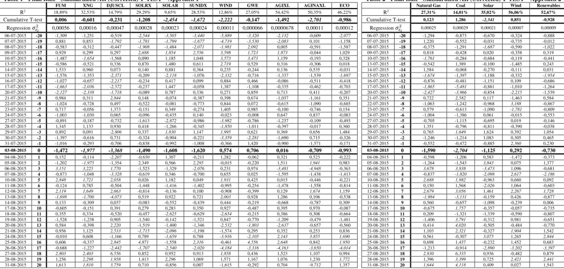
7 Numbers in italic represent test statistics that are significant, at least, on the 10% significance level. Table 1 - Final Rule - Standardized AR (Corrected) T-TEST – Approach 17
FUM XNG DJUSCL SOLRX SOLAR SUNIDX WIND GWE AGIXL AGINAXL ECO
R2 18,89% 32,53% 14,79% 29,29% 9,65% 28,53% 12,86% 27,05% 54,42% 50,35% 46,22%
Cumulative T-test 0,006 -0,601 -0,231 -1,208 -2,454 -1,672 -2,222 -0,147 -1,492 -2,701 -0,986 Regression𝜎𝜀2𝑖 0,00056 0,00016 0,00047 0,00028 0,00023 0,00024 0,00011 0,000066 0,0000678 0,00011 0,00012
06-07-2015 -20 -1,309 -1,251 -0,519 -2,544 -3,505 -3,440 -5,889 -3,320 -2,132 -0,609 -2,077 07-07-2015 -19 0,881 0,853 -1,792 -1,781 -1,799 -1,677 -4,719 -3,530 -2,083 0,101 -1,158 08-07-2015 -18 -0,583 -0,312 -0,447 -1,908 -1,484 -2,071 -1,981 2,092 0,005 -0,591 -1,587 09-07-2015 -17 0,929 0,299 0,297 2,688 1,854 2,556 3,598 1,723 1,873 -0,044 1,029 10-07-2015 -16 -1,487 -1,654 -1,568 0,090 1,185 1,048 3,573 3,473 1,159 -0,193 0,328 13-07-2015 -15 -0,586 -0,521 0,336 0,870 1,480 0,611 2,719 0,529 0,316 -0,306 0,018 14-07-2015 -14 1,533 0,960 0,073 0,140 0,881 0,364 0,235 -0,244 0,136 0,535 -0,031 15-07-2015 -13 -1,576 -1,353 -2,371 -0,209 -2,118 -1,076 -2,332 -0,716 -1,337 -1,539 -1,697 16-07-2015 -12 -1,027 -0,657 -2,217 -0,234 0,417 0,099 0,884 0,466 -0,086 -0,511 -0,418 17-07-2015 -11 -1,663 -2,036 -2,572 -0,237 1,447 -0,058 1,387 -1,108 -0,335 -0,462 -0,703 20-07-2015 -10 -2,127 -2,338 -1,718 -0,089 0,787 0,336 0,271 0,859 0,713 0,411 -0,207 21-07-2015 -9 0,984 0,311 2,844 0,148 -0,074 -0,387 0,398 0,674 -1,037 -1,161 0,351 22-07-2015 -8 -1,024 -0,728 0,497 -0,522 -0,081 -0,773 0,844 0,072 -0,615 -1,090 -0,685 23-07-2015 -7 0,717 -0,056 1,373 -0,151 0,349 -0,274 1,405 0,985 -0,100 -0,746 0,154 24-07-2015 -6 -1,003 -1,030 0,065 -0,096 -0,435 0,140 -0,023 -0,008 0,647 0,837 -0,083 27-07-2015 -5 -0,891 -0,187 -0,732 -1,613 -2,872 -0,986 -3,982 -0,786 -1,237 -0,109 -0,493 28-07-2015 -4 1,345 1,133 0,930 0,418 -1,266 -0,345 -1,850 -1,011 -0,397 -0,017 0,360 29-07-2015 -3 0,892 0,091 -2,806 0,337 1,830 1,147 1,995 0,621 0,369 0,656 1,484 30-07-2015 -2 -1,397 -0,616 0,731 -0,324 -0,904 -0,221 -3,359 -2,281 -1,690 0,715 -0,326 31-07-2015 -1 -1,016 -0,293 -0,706 -0,838 -0,992 -1,008 -0,366 1,420 -0,900 -1,571 -0,171
03-08-2015 0 -1,472 -1,977 -3,368 -1,490 -1,608 -1,620 0,574 0,706 0,016 -0,709 -0,993
04-08-2015 1 0,152 -0,114 -2,207 -0,650 1,307 -0,211 1,282 -0,062 0,321 0,523 -0,222 05-08-2015 2 -1,202 -1,975 -1,354 2,349 0,566 2,295 -0,015 -0,220 1,511 1,941 0,983 06-08-2015 3 3,151 3,225 1,770 -1,523 -1,329 -2,076 0,231 0,974 -3,481 -4,948 -0,363 07-08-2015 4 -0,873 -1,048 -3,328 -0,619 0,346 -0,700 0,655 0,025 -1,595 -1,438 -1,413 10-08-2015 5 2,848 1,721 2,058 0,026 1,182 0,049 1,931 0,425 0,015 -0,446 -0,221 11-08-2015 6 -0,124 0,785 -0,504 -1,448 -1,416 -1,402 -0,995 -0,254 -1,478 -1,558 -0,814 12-08-2015 7 2,119 1,649 2,663 -0,814 -0,136 0,100 -0,908 -0,399 0,129 1,674 1,159 13-08-2015 8 -1,698 -1,700 -4,073 0,519 0,922 0,721 2,003 0,928 1,286 0,106 -0,538 14-08-2015 9 0,133 -0,309 0,037 -0,083 -0,552 -0,439 0,444 -0,219 -0,668 -0,787 0,309 17-08-2015 10 -0,605 -0,151 0,391 0,279 0,283 0,350 0,927 -0,487 0,395 0,970 -0,087 18-08-2015 11 0,355 0,334 -0,520 -0,457 -2,625 -0,629 -2,654 -0,215 0,386 0,308 -0,664 19-08-2015 12 -1,528 -1,238 0,905 -1,540 -0,142 -1,521 0,847 -0,770 -1,209 -0,479 -1,481 20-08-2015 13 0,584 -0,398 2,220 -1,519 -1,400 -1,346 -2,532 -1,803 -2,637 -0,657 -0,560 21-08-2015 14 0,956 1,125 2,533 -1,715 -2,096 -1,198 -1,574 0,295 0,352 0,253 0,836 24-08-2015 15 -0,010 0,608 -1,166 0,789 -1,659 0,788 -3,916 -2,105 2,143 3,855 1,690 25-08-2015 16 0,606 -0,337 2,845 4,871 -1,558 2,316 -0,461 4,556 2,648 0,842 1,950 26-08-2015 17 -0,688 -1,227 -2,442 -1,707 -2,540 -2,020 -4,184 -3,316 -4,163 -3,650 -4,014 27-08-2015 18 2,803 2,403 6,556 0,852 0,952 0,913 1,858 0,436 1,523 1,107 0,994 28-08-2015 19 1,256 2,298 1,958 1,413 2,296 1,069 1,571 1,167 1,076 1,230 1,772 31-08-2015 20 1,613 1,810 3,759 0,710 -0,856 0,007 -1,615 -0,292 0,704 -9,712 1,357
Table 2 - Final Rule - Standardized AR (Corrected) T-TEST – Approach 2
Natural Gas Coal Solar Wind Renewables
R2
27,31% 14,01% 35,02% 56,06% 52,67%
Cumulative T-test 0,123 1,286 -2,341 0,851 -0,928
Regression𝜎𝜀2𝑖 0,00025 0,00029 0,00021 0,00007 0,00009 06-07-2015 -20 -1,294 -0,873 -0,670 -0,324 -0,888 07-07-2015 -19 1,220 -0,552 -0,031 -0,735 -0,012 08-07-2015 -18 -0,375 -1,291 -1,687 -0,590 -1,022 09-07-2015 -17 0,818 -0,428 0,020 -0,358 0,319 10-07-2015 -16 -1,761 -0,284 -0,684 -0,119 -0,441 13-07-2015 -15 -0,542 1,389 -0,100 -1,485 0,243 14-07-2015 -14 1,584 -0,068 -0,270 -0,111 0,031 15-07-2015 -13 -1,674 -1,397 -1,188 -0,332 -1,954 16-07-2015 -12 -0,876 -0,481 -1,151 0,109 -0,686 17-07-2015 -11 -1,865 -5,481 -0,881 -1,010 -1,264 20-07-2015 -10 -2,427 -3,966 -0,854 -2,215 -1,539 21-07-2015 -9 0,722 2,582 0,117 -1,463 0,584 22-07-2015 -8 -1,063 -1,242 -0,968 3,188 -0,867 23-07-2015 -7 0,579 -0,613 -1,090 -1,781 -0,809 24-07-2015 -6 -1,004 -1,386 0,061 -0,015 -0,553 27-07-2015 -5 -0,705 -1,115 -0,695 0,019 -0,146 28-07-2015 -4 1,351 -0,796 -0,811 -0,390 -0,038 29-07-2015 -3 0,765 1,649 1,624 0,392 1,054 30-07-2015 -2 -1,246 -1,214 1,083 0,305 0,465 31-07-2015 -1 -0,552 -0,472 -0,885 2,360 0,230
03-08-2015 0 -1,590 -2,704 -1,125 0,292 -0,730
25 of 25
Patell and BMP Statistics:
Patell’s statistic focus on SAR assuming no event-induced variance and no
cross-sectional correlation among securities while BMP’s statistic “relaxes the no-volatility-impact, and estimates the (common) event-day-volatility cross-sectionally with the usual sample standard deviation” (Kolari and Pynnöonen, 2010).
Patell statistic8
𝑃𝑎𝑡𝑒𝑙𝑙 =√(𝑚−2)/(𝑚−4)𝐴̅√𝑛 (13)
Adjusted Patell statistic9
𝐴𝑑𝑗𝑢𝑠𝑡𝑒𝑑 𝑃𝑎𝑡𝑒𝑙𝑙 = 𝐴̅√𝑛
√(𝑚−2)/(𝑚−4)√1+(𝑛−1)𝑟̅ (14)
Cumulative Adjusted Patell10
𝑧𝑃𝑎𝑡𝑒𝑙𝑙 =√𝑛1 ∑ 𝑆𝐶𝑆𝐴𝑅𝑖
𝐶𝑆𝐴𝑅𝑖
𝑛
𝑖=1 ∗ √1+(𝑛−1)𝑟̅1 (15)
BMP statistic11
𝐵𝑀𝑃 =𝐴̅√𝑛𝑠 (16)
Adjusted BMP statistic12
𝐴𝑑𝑗𝑢𝑠𝑡𝑒𝑑 𝐵𝑀𝑃 =𝑠 𝐴̅√𝑛
𝐴√1+(𝑛−1)𝑟̅ (17)
Cumulative Adjusted BMP statistic13
𝑧𝐵𝑀𝑃 = √𝑛 ∗𝑆𝑆𝐶𝐴𝑅̅̅̅̅̅̅̅̅
𝑆𝐶𝐴𝑅 ̅̅̅̅̅̅̅̅√ 1−𝑟̅ 1+(𝑛−1)𝑟̅ (18) 8
𝐴̅ =1𝑛∑𝑛𝑖=1𝑆𝐴𝑅𝑖,𝑡 𝑆𝐴𝑅𝑖,𝑡=𝑆𝐴𝑅𝑖,𝑡
𝐴𝑅𝑖,𝑡
𝑀𝑖= Count of non-missing return values in the estimation window for the firms. 𝑛 = Count of the number of firms.
9
𝑟̅ = average of the sample correlations of estimation period abnormal returns
10
𝐶𝑆𝐴𝑅𝑖= ∑𝑡=𝑇𝑇2 1+1𝑆𝐴𝑅𝑖,𝑡 𝑆𝐴𝑅2𝑖,𝑡= 𝑆𝐴𝑅2 𝑖∗ (1 +
1 𝑀𝑖+
(𝑅𝑚,𝑡−𝑅̅𝑚)2
∑𝑇1𝑡=𝑇0(𝑅𝑚,𝑡−𝑅̅𝑚)2) 𝑆𝐶𝑆𝐴𝑅𝑖
2 = (𝑇
2− 𝑇1) ∗𝑀𝑀𝑖𝑖−2−4 𝑇1= Starting day of the event window 𝑇2= End day of the event window
11
𝑠2= 1
𝑛−1∑ (𝐴𝑛𝑖=1 𝑖− 𝐴̅)2
12
𝑠𝐴2= 𝑠
2
1−𝑟̅
13
𝑆𝐶𝐴𝑅 ̅̅̅̅̅̅̅ =1
𝑛∑𝑛𝑖=1𝑆𝐶𝐴𝑅𝑖 𝑆𝑆𝐶𝐴𝑅̅̅̅̅̅̅̅̅2 = 1
𝑛−1∑ (𝑆𝐶𝐴𝑅𝑛𝑖=1 𝑖− 𝑆𝐶𝐴𝑅̅̅̅̅̅̅̅)2
𝑆𝐶𝐴𝑅2 𝑡= 𝑆𝐴𝑅2𝑖∗ (𝐿𝑖+ 𝐿2𝑖 𝑀𝑖+
(∑𝑇𝑡=𝑇2 1+1(𝑅𝑚,𝑡− 𝑅̅𝑚)) 2
∑𝑇𝑡=𝑇1 0(𝑅𝑚,𝑡− 𝑅̅𝑚)2 )