M. A. Zermani 1, E. Feki 2 and A. Mami 3
1
Department of Physics, Faculty of Science, Mathematics, Physics and Natural of Tunisia, Tunis, Campus Universities 2092 El Manar,Tunisia
Abstract
In this paper, we focused on a design of an algorithm for decoupling multivariable systems based on generalized predictive control (DGPC). Two techniques are developed and compared for decoupling of TITO (Two-Input, Two-Output) processes. The first method is based on adding compensators between the upper and lower control paths. According to the second method, we use an adaptive error weighting factor in cost function in order to reduce coupling between control loops. The method is applied in simulation to the multivariable control of incubator system.
Keywords: Incubator Process, Decoupling Predictive Control, Optimal decoupling, Tuning error weighting factor.
1. Introduction
The progressive technological evolution of servo controlled incubators has created a need constantly to increase the capacity of these incubators to reach and maintain the desired temperature[1][2]. Consequently, the temperature is one of the most important factors that must be maintained with minimal variation to keep constant internal temperature. According to the study conducted in the Center Maternity and Neonatology of Tunisia (CMNT)[3], we noted that the infant is often exposed to disruption because of successive interventions of the medical team, which requires the presence of a controller more efficient. The newest incubators, such as Drager Isolette C2000 [3][4], uses a controller based on Proportional- Integral- Derivative (PID) to control internal temperature and a ON-OFF controller to increases the moisture by vaporization water [1][15]. However, the design of an active humidification system, modeling and implementation of a controller for a multi input multi-output, highly coupled constitute a real scientific challenge[1][15][16][17].. The contribution of this paper
focused on the development of a decentralized predictive decoupling controller for heating and humidification systems. Two decoupling methods designed around GPC controller were developed and compared.
The paper is structured as follows: The section 2 is devoted to present decentralized generalized predictive control with constraint. In section 3, we propose the first method of decoupling based on adding compensators between the upper and lower control paths. In second method we develop an adaptive error weighting factor in in order to reduce coupling between control loops. In section 4, computer simulations are conducted shown how the controller parameters of the two predictive control algorithms can be adapted to decrease the coupling effect between controlled variables (temperature and humidity) of incubator system.
2. Decentralized Predictive control
take into count this structure Fig. 1, for the conception of the decoupling predictive control.
y1
yn yc1
ycn
Procédé u1
un C1
Cn
. . .
. . .
Fig. 1 Structure of decentralized control (or distributed)
2.1 Process model
The synthesis of the generalized predictive controller (GPC) suggested by (Clarke et al, 1987; Clarke, 1988) [7],[8]. This method was used successfully in industrial applications of various forms [9],[10],[11]. The approach of generalized predictive control is based on a dynamic model of type ARIMAX (Auto Regressive Integrated Moving Average with eXternal inputs), given by:
1 1 1
1
( ) ( ) ( ) ( ) ( 1) ( ) .
( )
i
d i
i i i i i
e k
A z y k z B z u k C z
z −
− − −
−
= − +
∆ (1) Where i is the number system, y ki( ) is the system output,u ki( )is the system input,e ki( )is the uncorrelated
random sequence, 1 1
(z−) 1 z−
∆ = − corresponds to an integral action. Its presence in the direct channel allows a zero error in steady state value. 1
( ) i
A z− , 1
( )
i
B z− and 1
( )
i
C z− are polynomials.
1 1 2
1 2
1 1 2
0 1 2
1 1 2
1 2
( ) 1 ,
( ) ,
( ) 1 .
i
i
na
i nai
nb
i nbi
nci
i nci
A z a z a z a z
B z b b z b z b z
C z c z c z c z
−
− − −
−
− − −
− − − −
= + + + +
= + + + +
= + + + +
(2)
With na nb et nci, i i indicate the respective order of these polynomials.
The generalized predictive control based on the minimization of a quadratic criterion on a sliding horizon, which involves a term related to the difference between the predicted output sequence and the sequence of future control [12].
The criterion is given by:
2 2
1
ˆ
[ ( ) ( )] ( 1)
i ci
i i
HP N
i yi t N C i ui t i
J =λ
∑
= y k t+ −y k t+ +λ∑
= ∆u k t+ − (3)with ˆ ( )y ki is the output value predicted at time k, ( )
i
C
y k is the set points values at time k,∆u ki( ) is the increment of control at time k, Ni is the minimum prediction horizon, HPi is the maximum prediction horizon,
i
c
N is the control horizon, λui is the control weighting factor andλyiis the error weighting factor.
2.2 Prediction of the system output:
Consider the output expressed by (1) the output at time instant (k+t) will be:
1 1
1 1 1
( ) ( )
( ) ( 1) ( )
( ) ( ) ( )
i i
i i i i
i i
B z C z
y k t u k t d e k t
A z A z z
− −
− − −
+ = + − − + +
∆ (4)
By applying the Euclidean algorithm on the second term of (4) we get
1 1
1
1 1 1 1
( ) ( )
( )
( ) ( ) ( ) ( )
t
i t
t
i i
C z G z
L z z
A z z A z z
− −
− −
− ∆ − = + − ∆ − (5)
After using (4) and (5), we assume that the term related to the disturbance is zero, the optimal predictor of the output is:
1 1 1 1
1 1
( ) ( ) ( ) ( )
ˆ ( ) ( 1) ( )
( ) ( )
t i t
i i i i
i i
L z B z z G z
y k t u k t d y k
C z C z
− − − −
− −
∆
+ = + − − + (6)
A second Diophantine equation decompose the predictor in two terms: a term based on the current output, old orders, the system output and a second term dependent on future orders.
1 1
1
1 1
( ) ( )
( )
( ) ( )
i
t d
i t
t
i i
z R z
H z z
C z C z
σ − −
− + −
− = + − (7)
With:
1 1 1
( ) ( ) ( ) i z L zt B zi
σ − = − − (8)
The optimal predictor of the output is:
1 1
1 1
1
1 1
ˆ ( ) ( ) ( ) ( 1)
( ) ( )
( ) ( ) ( 1)
( ) ( )
i t i i
t t
i i
i i
y k t H z z u k t d
G z R z
y k z u k
C z C z
− −
− −
−
− −
+ = ∆ + − − +
+ ∆ −
(9)
Where ( 1)
t
H z− ( 1)
t
G z− R zt( −1)and 1
( ) t
* *
ˆ
ˆ ˆ ˆ
i i i i i i i
Y =H∆ +U G Y + ∆R U (10)
The vector of the predicted outputs ˆYi is the sum of the predicted forced ˆ
i i
H∆U and free responsesG Yˆi i*+ ∆R Uˆi i* with:
ˆ [ (ˆ 1/ ) ,ˆ( 2 / ) ˆ( / )] ,T
i i i i i
Y= y k+ k y k+ k y k HP k+ (11)
* [ *( ) , *( 1) *( )] ,T
i i i i i
Y = y k y k− y k−na (12)
[ ( ) ( 1)] ,T
i i i Ci
U u k u k N
∆ = ∆ ∆ + − (13)
* * *
[ ( 1) ( 1)] ,T
i i i
U u k u k nbi di
∆ = ∆ − ∆ − − + (14)
1 1
1
ˆ [ ( ) ( )] ,
i i i
T
i d HP d
G = G+ z− G + z− (15)
1 1
1
ˆ [ ( ) ( )] ,
i i i
T
i d HP d
R = R+ z− R + z− (16)
0
1 0
1 2
0 0
0 ˆ
i i i Ci
i
HP di HP di HP di N
h
h h
H
h − − h − − h − −
=
(17)
Where:
* *
1 1
( ) ( 1)
( ) , ( 1) ,
( ) ( )
i i
i i
i i
y k u k
y k u k
C z− C z−
∆ −
= ∆ − =
and (( ))
( )
ˆ
D IM ( ) H P d , na d 1 ,
ˆ
D IM ( ) H P d , nb d 1 ,
ˆ
D IM ( ) H P d , N ,
i i i i i
i i i i i
i i i Ci
G
R
H
= − + −
= − + −
= −
denote the dimension of ˆGi, ˆRiand ˆHi, respectively.
2.3 Law order
We write the criterion J in matrix form
ˆ ˆ
[ ( ) ( )] [ ( ) ( )] ( ) ( )
i i
T T
i i C i C ui i i
J=Y k Y k− χ Y k Y k− + ∆λ U k ∆U k (18)
With:
[ ( ) ( )]
i
Ci C i Ci i i
Y = y k+d y k+HP+d (19)
The optimal vector∆Ui is:
(ˆ ˆ ) 1 ˆ ˆ
Ci
T T T
i i i i ui N i i
U H χH λ I − H Y
∆ = + (20)
The optimal control law is derived from analytical minimization of the previous cost function. Only the first control value is finally applied to the system.
( ) ( ) ( 1).
i i i
u k = ∆u k +u k− (21) Which∆u ki( )is the first element of the vector∆Uiand
C
N
I is diagonal matrix of size NCi*NCiandχiis diagonal matrix of sizeHPi−di*HPi−di
0
1 0
,
0 1 0
C i
yi
N i
yi I
λ χ
λ
= =
(22)
2.4 Constraints formulation
Generally, the constraints imposed on the control signal and its increment are described by inequalities forms
( )
( )
( )
( )
min i max
i i i
u k u k u k k
su u k su
≤ ≤ ∀
− ≤ ∆ ≤ (23)
Where
u
min ,u
max andsu
i are respectively lower threshold, the upper threshold and derivative threshold of the control inputs. On the horizon controller HCi can be written:( )
(
)
(
)
,
1 ,
1 ,
i i i
i i i
i i i i
su u k su
su u k su
su u k H C su
− ≤ ∆ ≤
− ≤ ∆ + ≤
− ≤ ∆ + − ≤
(24)
Or in the condensed form:
1 1
,
i I
U I
β
β
−
∆ ≥
− −
(25)
With I is identity matrix of dimension (HCi, HCi),
i
U
∆ andβ1are two vectors with the same dimensions HCi :
[
]
( )
(
)
1 ,
, , 1
T
i i
T
i i i i
su su
U u k u k HC
β =
∆ = ∆ ∆ + −
(26)
( )
( )
( )
( )
( )
( )
( )
( )
( )
(
)
( )
min max
min max
min max
1 1 ,
1 1 1 ,
1 1 1 ,
i i i
i i i i
i i i i i
u u k u k u u k
u u k u k u k u u k
u u k u k u k HC u u k
− − ≤∆ ≤ − −
− − ≤∆ +∆ + ≤ − −
− − ≤∆ + ∆ + − ≤ − −
(27)
Or in the condensed form:
(
)
(
)
2
3
1 , 1
i
k W
U
k W
β β
−
∆ ≥
− − −
(28)
With
β
2T etβ
3T are two vectors with the same dimensions HCi:( )
( )
( )
( )
( )
( )
2 min min
3 max max
1 1 1 ,
1 1 , , 1 .
T
i i
T
i i
k u u k u u k
k u u k u u k
β β
− = − − − −
− = − − − −
(29)
And W is a matrix of dimension (HCi, HCi).
1 0 0
1 1 0 0
1 1 1
W
=
(30)
We can rewrite the two inequalities (3.25) and (3.28)
(
)
(
)
1
1
2
3
, 1
1
i
I I
U
k W
W k
β β β
β −
− −
∆ ≥
−
− − −
(31)
The problem of minimization of the criterion J with constraints is writing:
i i
i
^ ^
T T
i
i C i i C ui i i
U
minJ [Y(k) Y (k)] [Y(k) Y (k)] U(k) U(k)
∆ = − χ − +λ ∆ ∆ (32)
( ),
i
U k
ψ∆ ≥φ (33) With:
(
)
(
)
2 3
1 1
, , ,
( ) , , 1 , 1
T T T
T T T T T
I I W W
k k k
ψ
φ β β β β
= − −
= − − − − −
(34)
The minimization of this criterion cannot be performed analytically. The synthesis of the control law amounts to solving an optimization problem of a quadratic criterion under constraints like inequalities. During the simulations
proposed subsequently, the determination of the optimal control sequence is done using the function "fmincon" of Matlab™.
3. Decoupling Control Design for TITO
System
3.1 Optimal decoupling control
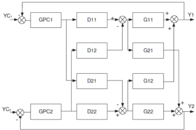
The system design of GPC decoupling control based on ideal decoupler is presented in Fig. 2
Fig . 2 Configuration of GPC decoupling control system.
D12, D21 and D22 are the decoupling compensation segment.
The advantage of using a decoupling controller over a multivariable GPC is that decoupling and tuning are separate tasks. The decoupling methods use usually in the multivariable coupled process includes diagonal matrix method, unit matrix method and feed-forward compensation method. In this work we interested to the diagonal matrix method to decouple the incubator system. In Fig. 2 G is dynamic transfer function and D is the decoupling matrix. To simplify decoupling process D11= D22=1.
The transfer functions are:
1 11 12 21 12 11 12 1
2 21 22 21 22 21 12 2
Y(k) G (z) G (z).D (z) G (z) G (z).D (z) U(k) Y(k) G (z) G (z).D (z) G (z) G (z).D (z) U (k)
+ +
=
+ +
(35)
The decoupling conditions are obviously:
12 11 12
21 22 21
G G D 0 G G D 0
+ =
+ =
(36)
11
22
21 21
22
12 12
11
D 1 D 1 G D
G G D
G
=
=
−
=
−
=
(37)
The decoupling dynamic transfer function is:
12
11 d
21
22
G (z) 0 G (z) G (z)
G (z) 0
G (z)
=
(38)
However, these controllers cannot fully solve problems with strong interactions among control loops. Adding interaction compensators to controllers can improve control [6], but in some systems, because of improper delay structure or model mismatch, interaction compensators are not applicable.
3.2 Decoupling by tuning weighting factor based on
error observation
To overcome the drawback of the previous method we present a new approach to decoupling the structure of the decoupling control which is also described in the figure 3.
G11
G22 G21 G12
GPC2 GPC1
weighting factor
e1(k)
Y1
Y2
-+
+
yc1
yc1(k) -yc1(k-1) =
e2(k)=yc2(k) -yc2(k-1)
yc2
noise
noise
Fig. 3 Control structure of generalized predictive control with weighting factor adjusting.
The main idea of decoupling controller is the following [14]: when some reference changes its value (for example: set-point of y1) controller firstly increases only λy2 in the
second loop, and then calculate optimal control vector (32) and (33).
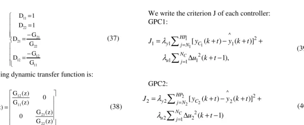
We write the criterion J of each controller: GPC1:
1 1 1
^
2
1 1 1
2
1 1 1
[ ( ) ( )]
( 1),
C
HP y j N C
N
u j
J y k t y k t
u k t
λ λ
=
=
= + − + +
∆ + −
∑
∑
(39)GPC2:
2 2 2
^
2
2 2 2
2
2 1 2
[ ( ) ( )]
( 1)
C
HP
y j N C
N
u j
J y k t y k t
u k t
λ λ
=
=
= + − + +
∆ + −
∑
∑
(40)This control vector would minimize output deviation caused by reference changes. Values λyi are evaluated from equation:
( )
m ri
yi j 1 1 C j
K
1 y (k)
M q−
=
= + ∆
λ
∑
(41)
ri
K : maximum error weight in j loop,
C j
y
∆ : reference change on j input,
( )
1M q− : Polynomial of q−1defined by designer.
4. Application to an incubator system
4.1 Modeling
The incubator system include an AC-powered heater, a fan to circulate the warmed air, a container for water to add humidity and access ports for nursing care. With the technology available currently, incubators use microprocessor-based control systems to create and maintain the ideal microclimate for the preterm neonate.
Fig. 4 Schematic of the incubator process with experimental arrangement for active humidification to control temperature and Humidity.
An experimental method is proposed for modeling of the TITO system. The incubator system has two inputs and two outputs.
The inputs to the system are:
U1: control signal applied to the heater, U2: control signal applied to the nebulizer. The outputs are:
Y1: temperature value output signal, Y2: humidity level output signal.
The transfer function matrix of the incubator system can be expressed as follow:
1 11 12 1 1 1
2 21 22 2 2 2
Y(k) G (z) G (z) U (k) C (z) 0 e (k) Y (k) G (z) G (z) U (k) 0 C (z) e (k)
= +
(42)
G12
G11
G22 G21
+ +
+ +
T
H U1
U2
C1
e1
C2
e2
+
+
Figure 5. Input-output model of incubator system.
G11 is a transfer function showing the relation between input U1 and output y11. Likewise, G12 is the transfer function that shows the effect of input U2 to output y12, G21 indicates the effect of input U1 to y21; G22 indicates the effect of input U2 to output y22.
The transfer functions of the various subsystems are described as follow:
dij 1
ij
ij 1 i
ij
z B (z ) y (k) U (k 1)
A (z )
− −
−
= − (43)
( )
( )
( )
( )
1 11 12 1 1
2 22 21 2 2
Y (k) y k y k C e (k) Y (k) y k y k C e (k)
= + +
= + +
(44)
Where i and j are the level indices i, j = {1, 2} andAij,Bij and Cijare polynomials:
1 1 2 na
ij 1 2 na
1 1 2 nb
ij 0 1 2 nb
1 1 2 nc
i 1 2 nc
A (z ) 1 a z a z a z B (z ) b b z b z b z C (z ) 1 c z c z c z
− − − −
− − − −
− − − −
= + + + +
= + + + +
= + + + +
(45)
We present the multivariable system as matrix form:
1 1
11 11 12 12
1 1
11 11
11 12
1 1
21 22 21 21 22 22
1 1
21 22
10 1
1 2
32
( ) ( )
( ) ( )
( )
( ) ( )
( ) ( )
(5.9746e-004+5.9412e-004 )
0
1- 0.3467 -0.6463z
z (1.3698e-004-4.193
d d
d d
B z B z
z z
A z A z
G G G z
G G B z B z
z z
A z A z
z z
z
− −
− −
− −
− −
− −
− −
− −
− −
−
= =
=
1 3 1
1 2 1 2
.
0e-004z ) z (0.00203+0.00088z )
1 0.28321z 0.7133z 1 0.5091z 0.4262z
− − −
− − − −
− − − −
(46)
The temperature variation is almost not related to the change in moisture level (G12=0), and this weak relation can be modeled as a disturbance to the system. The other components are simply modeled with a second order system with a time varying delay.
4.2 Computer simulations of optimal and weighting
factor decoupling of incubator system
The principal parameters are set as follows; the prediction horizon isHP1=HP2=20, the control horizon is NC1=NC2 =1, the weighting factors of the control
increments are λu1=0.0026, λu 2=0.6273 and the error
weighting factor is λy1=λy2=1. The coupling effect was
simulated with constraints and at sampling time T=20 seconds.
Chosen constraints 1 2
0% 100%
0% 100%
U
U
≤ ≤
≤ ≤
To overcome the drawback of the previous method we present the simulation result of decoupling by tuning weighting factor which λy2 is evaluated from equation (41)
With :
( )
1 12
M q− = −1 0.989q ,− Kr = 5
200 400 600 800 1000 1200 1400 1600 1800 2000
10 15 20 25 30
Samples
T
em
p
er
at
u
re
(°
C
)
Temperature output Set-point
Fig. 6 Simulation result of set-point tracking temperature for predictive decoupling control.
200 400 600 800 1000 1200 1400 1600 1800 2000
60 65 70 75 80
Samples
H
u
m
id
it
y
(%
)
Humidity with adaptive weighting factor Humidity with optimal decoupling Set-point
Fig. 7 Compared result of set-point tracking humidity with tuning weight factor by reference change and by adding interaction compensators .
200 400 600 800 1000 1200 1400 1600 1800 2000 0
20 40 60 80
Samples
W
e
ig
h
ti
n
g
f
ac
to
r
λy2
Fig. 8 Evolution of the weighting factor synchronized with change set point.
200 400 600 800 1000 1200 1400 1600 1800 2000 0
50 100 150 200
Samples
C
o
n
tr
o
l
(%
)
Contorl Humidity with adaptive weighting factor control Control Humidity with optimal control
Control Temperature
Fig. 9 Simulation results of temperature and humidity control with decoupling in incubator system
by compensation block. In Fig 8, we present the evolution of the weighting factor which is synchronized with reference change. Fig. 9 illustrates the simulation results of temperature and humidity control with two decoupling method in incubator system.
Proposed concept of tuning weighting allows to simple decoupling controller and it is applicable to all multivariable controllers based on some cost function minimization.
5. Conclusions
In this paper, we have developed a multivariable control algorithm based on decoupled predictive control, which takes into account natural constraints on the actors (the heater and nebulizer). Simulations results have been demonstrated that decoupling by tuning weighting factor with synchronization in set-point change is simpler for implementation than decoupling by adding interaction compensators.
Main advantage of the weight decoupling method is its simplicity and computational burden, which makes it more suitable as adaptive controller for complex system than others decoupling method.
References
[1]F. Telliez, V. Bach, S. Delanaud, H. M. Baye, A. Leke, A. Apdoh and M. Abidiche, “Influence du niveau d’humidité de l’air sur le sommeil du nouveau-né en incubateur”, RBM. Revue européenne de biotechnologie médicale, vol.21, pp.171-176, 1999.
[2] J.L. Costa, C.S. Freire, B.A. Silva, M.P. Cursino, R. Oliveira, A. M. Pereira and F.L. Silva, “Humidity control system in newborn incubator”, Fundamental and Applied Metrology, 2009.
[3]M. A. Zermani, E. Feki and A. Mami, “Application of Adaptive Predictive Control to a Newborn Incubator”, American J. of Engineering and Applied Sciences, 4 (2), pp. .235-243, 2011.
[4]Drager Medical Systems, “Drager isolette c2000 infant incubator brochure”, April 2004.
[5]A. Benhammou. Contribution à l’étude de la commande adaptative décentralisée des systèmes interconnectes. Thése de troisième cycle, L.A.A.S, Toulouse, France, 1988. [6]E. Gagnon. Simplified, ideal or inverted decoupling. ISA
Trans.,vol 37 , pp.265–276, 1999.
[7] D. W. Clarke, C. Mohtadi and P. S. Tuffs, “Generalized Predictive Control - Part I and II”, Automatica, vol.23(2), pp. 137-160, 1987.
[8]D. W. Clarke, “Application of Generalized Predictive Control to Industrial Processes”, IEEE Control System Magazine, vol. 8, pp.49-55, 1988.
[9] Li, G., Stoten, D.P., Tu, J.-Y., “Model predictive control of dynamically substructured systems with application to a servohydraulically actuated mechanical plant”, IET Control Theory Appl., 2010, vol. 4, (2), pp. 253–264
[10] J. Richalet, D. O’Donavan, “Elementary Predictive Functional Control”, Springer Verlag, Berlin, 201-105, 2009. [11] J. T. J. Richalet, A. Rault and J. Papon, “Model predictive heuristic control: Applications to industial processes”, Automatica, vol.14, pp. 413–428, 1978.
[12] C. C. Tsai and C. H. Huang, “Model reference adaptive predi- ctive control for a variable-frequency oil-cooling machine”, IEEE Trans. Ind. Electron, vol. 51(2), pp. 330-339, 2004.
[13] D. W. Clarke, C. Mohtadi and P. S. Tuffs, “Generalized Predictive Control - Part I and II”, Automatica, vol. 23(2), pp. 137-160, 1987.
[14] Bego, O. Peric, N. I. Petrovic, “Decoupling multivariable GPC with reference observation”, 10th Mediterranean Electrotechnical Conference , vol.2, pp.819 – 822, 2000. [15] M. A. Zermani, E. Feki and A. Mami, “Application of
Genetic Algorithms in identification and control of a new system humidification inside a newborn incubator”, International Conference on Communications, Computing and Control Applications, pp. 1-6, 2011.
[16] V. Hurgoiu. Thermal regulation in preterm infant. Early Hum. Dev, 28 :1˝ U5, 1992.