V. A. Sujan
Cummins Engine Company Air Handling and Combustion Control Division 500 Jackson Street, 47201 Columbus, IN. USA [email protected]
M. A. Meggiolaro
PUC-Rio Departamento de Engenharia Mecânica Rua Marquês de São Vicente, 225 - Gávea 22453-900 Rio de Janeiro, RJ. Brazil [email protected]
Model Predictive Disturbance
Rejection during Cooperative Mobile
Robot Assembly Tasks
This paper addresses the problem of disturbance compensation for the successful assembly of structures by mobile field robots. A control architecture, consisting of a linear PID joint controller with model predictive feed-forward compensation for mobile base motions and interactive-force disturbance rejection is discussed. Object insertion is achieved by predicting environment-object contact states and motions are planned in the direction of least resistance. Issues addressed include dynamic modeling of multiple cooperative robots, control architecture design and stability analysis, and environment-object contact state prediction. Simulation results show the effectiveness of the control architecture. Keywords: Cooperative robots, model predictive control, robot assembly
Introduction
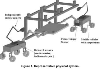
Future mobile field robotic systems, such as planetary and terrestrial mission robots, will be required to perform complex tasks (Huntsberger, 1997; Shaffer and Stentz, 1992). Planetary robots will be used to collect rock samples, to build infrastructures, and explore complex terrains. Tasks for terrestrial field robots may include explosive ordinance removal, de-mining and handling hazardous waste, and environment restoration (Baumgartner et al., 1998; Huntsberger, 1997; Osborn, 1989; Shaffer and Stentz, 1992). Those will require the handling of relatively large objects, such as deploying of solar panels and sensor arrays, anchoring of deployed structures, movement of rocks, and clearing of terrain.An important goal of robotics research is to develop mobile robot teams that can work cooperatively in unstructured field environments, such as shown conceptually in Fig. 1 (Baumgartner et al., 1998; Huntsberger, 1997).
Each field robot may be equipped with a manipulator arm and sensors such as inclinometers, accelerometers, vision systems, and force/torque sensors. The control of such systems typically requires models of the environment and task. This paper addresses the problem of assembly (insertion) tasks performed by cooperative mobile robots in field environments.
Substantial previous research has been devoted to control and planning of cooperative 1robots and manipulators (Alur, 2000; Donald et al., 1997; Gerkey and Mataric, 2000; Khatib, 1995; Marapane et al., 1996; Mataric, 1998; Parker, 1995; Veloso and Stone, 1999). However, these results are largely inapplicable to mobile robots in unstructured field environments. The methods developed to date generally rely on assumptions that include: flat and hard terrain; accurate knowledge of the environment; little or no task uncertainty; and sufficient sensing capability. Additionally, researchers have developed several approaches to the single robot object insertion problem including motion in direction of least resistance, perturbation methods, petri-nets and event-based approaches, and remote compliance center modeling for contact state identification (Giraud and Sidobre, 1992; Hirai and Iwata, 1992; Kang et al., 1998; Kitagaki et al., 1993; Kittipongpattana and Laowattana, 1998; Lee and Asada, 1999; McCarragher and Asada, 1993; Shimokura and Muto, 1996; Xiao and Liu, 1998).
Little work has been done in addressing the problem of autonomous field robots cooperatively assembling structures. In
Paper accepted July, 2004. Technical Editor: José Roberto de França Arruda.
unstructured field environments the robot(s) needs to construct environment and task models from available sensory information.A number of problems can make this difficult. These include the uncertainty of the task in the environment, location and orientation errors in the individual robots, sensing occlusions, and external disturbances. Previously reported work has addressed problems due to environment and task sensing uncertainty and limitations (Sujan, 2002a; Sujan, 2002b; Sujan and Dubowsky, 2002).
This paper addresses the problem of disturbance compensation for the successful assembly of structures by mobile field robots. Disturbances may arise due to inter-robot and robot-environment interaction forces. Such disturbances can significantly degrade the performance of a manipulator. They may cause the manipulator to leave its prescribed path, saturate its actuators, and induce high stresses (both internal and external e.g. at the endpoint). Additionally, a critical element in task execution may be the stresses exerted by the system(s) on the structure elements and the environment. Therefore, these forces will have to be monitored and kept below a damage threshold during the entire task.
The control system proposed for manipulator control is a linear PID joint controller with model predictive feed-forward compensation for mobile base motions and interactive-force disturbance rejection. Object insertion is achieved by predicting environment-object contact states (from force/torque sensor readings) and motions are planned in the direction of least resistance. To model an appropriate controller for such a system, a dynamic model of this environment must be developed. Such a model will demonstrate the relationship between manipulator joint angles/positions, vehicle base motions and external end-point interactive forces.
Simulation results show the effectiveness of the control architecture. Without dynamic disturbance compensation in the control loop, the system is seen to fail. However, with dynamic disturbance compensation in the control loop, the robots are now able to predict the errors that would be introduced into the system due to external interaction forces, and succeed in task execution.
Nomenclature
bi = 3x1 unit vector along joint axis i, dimensionless
d = measured vehicle disturbance vector [xV, yV, θV]T
dxi, dyi, dzi = distance between the vehicle center of gravity and tire i in the x, y or z direction, m
F = measured manipulator endpoint external force, N
Fk = externally applied force [Fxk, Fyk, Fzk]T, N
Copyright 2004 by ABCM July-September 2004, Vol. XXVI, No. 3 /261
fV = vehicle damping feed-forward term (analytical)
ffr = measured contact friction force, N fn = measured normal contact force, N
g = gravitational acceleration vector [gx, gy, gz]T, m/s2 G = gravitational term, N or N⋅m
H = augmented inertia tensor of the manipulator-vehicle system
Hij = element (i, j) of the manipulator-vehicle system inertia matrix H
HM = augmented inertia tensor of the manipulator solely
h = augmented matrix of Coriolis and centrifugal coefficients of the manipulator-vehicle system
hijk= Christoffel’s three-index coefficient
hM = augmented matrix of Coriolis and centrifugal coefficients of the manipulator solely
I = moment of inertia, N⋅m2
J = manipulator Jacobian matrix
J(j) = column j of the manipulator Jacobian matrix
KD = derivative control gain KI = integral control gain KP = proportional control gain
Kx,y,z = linear stiffness in the x, y or z direction, kN/m
Kθ = angular stiffness, kN⋅m
l = link length, m
m = link mass, kg
Mj = externally applied moment [Mxj, Myj, Mzj]T, N⋅m p = position vector [xp, yp, 0]T of point p in Fig. 4, m Qi= generalized force on joint i, N
qi = generalized coordinate associated to joint i, m or deg
ri = position vector [xi, yi, zi]T of particle i, m ri,cj = vector of centroid of link j from ith frame, m
Sk = position vector [xSk, ySk, zSk]T where external force Fk is applied, m
T = total torque [Tx, Ty, Tz]T acting on point p in Fig. 4, N⋅m V = Lyapunov function
vc = linear velocity of link centroid, m/s
Greek Symbols
θ = angular displacement, rad Θ
Θ Θ
Θ = manipulator parameter vector [θ1, θ2, θ3]T ττττ = joint torque vector, N⋅m
ω ω ω
ωc = link angular velocity, rad/s
Subscripts
A relative to angular velocities D relative to derivative control d desired value
F relative to force control I relative to integral control i relative to manipulator joint i L relative to linear velocities P relative to proportional control v relative to vehicle center of gravity x relative to the x direction
y relative to the y direction z relative to the z direction
zmp relative to the zero moment point ~ estimation error
Control Algorithm Development
A feedback controller is characterized by not reacting to a disturbance before a control error has already occurred. But in many cases it is possible to measure the value of a disturbance before it gives rise to a control error. In model predictive control, disturbance rejection is accomplished by estimating the equivalent disturbance
of a system based on its dynamic model and the sensed disturbances. This is also known as feed-forward control, which takes control action in the manipulator to eliminate the impact of uncontrolled vehicle disturbances before any errors in the manipulator can be detected, see Fig. 2. Disturbance measurements are fed into a dynamic system model to account for the errors caused by them. The resulting dynamic disturbance commands are fed-forward and added to the basic controller commands to give the system control input. The basic joint-level controller considered here is a PID controller. To function effectively, such a system is dependent on an accurate dynamic model and low noise sensors. Degradation in the accuracy of the models and the disturbance measurements result in corresponding degradation of the controller.
Using a Lagrangian formulation, the dynamic models of the systems and task (represented in Fig. 1) are developed. These models account for robot base motion, compliance, and multi-robot interaction forces (see Fig. 3 for a planar representation). This method can be readily extended to model the closed chain dynamics of multiple cooperating robots. The primary steps involved in this process are now described.
Figure 1. Representative physical system.
manipulator dynamics
J−−−−1 joint
controller manipulator + base dynamic
model vehicle motion
sensors
mobile manipulator
kinematics disturbance compensation desired
endpoint position
actual endpoint position
+
+ +
endpoint error
joint error
−−−−
joint angles gravity
compensation
+
Figure 2. Block diagram of linear feed-forward compensation for dynamic disturbance rejection.
Step 1: Reduction of Suspension Compliance System
∑
∑
∑
∑
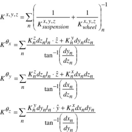
+ ⋅ = + ⋅ = + ⋅ = + = − − − − n n n n n x n n n y n n n n n n x n n n z n n n n n n y n n n z n n n z y x wheel z y x suspension z y x dy dx dy dx K y l dy K K dz dx dz dx K z l dz K K dz dy dz dy K z l dz K K K K K z y x 1 1 1 1 , , , , , , tan ˆ tan ˆ tan ˆ 1 1 θ θ θ (1)where xˆ, yˆ, zˆ are unit normal direction vectors for the x, y, z axes respectively, as shown in Fig. 3(a). Similar expressions may be derived for the 6 DOF damping terms.
x y z 2 , 1 p 1
q q2
. F1 F2 z x y
O1 O2
xV, yV, θθθθV
.
.
xV, yV, θθθθV
vehicle chassis
F
xV, yV, θθθθV
vehicle & suspension motion θθθθ1 θθθθ2 θθθθ3
m3, I3, l3
m2, I2, l2
m1, I1, l1
M, I
(a) (b)
Figure 3. Cooperative robot modeling. (a) Interacting mobile systems, (b) Individual robot with interaction forces
Step 2: Robot Model Lagrangian Dynamics
In general for a multi-DOF serial manipulator, the spatial equation of motion for the ith link is given by:
( )
in j n k k j ijk n j j ij i
i H q h q q G
Q − =
∑
+∑ ∑
+= =
=1 1 1
& & &&
F
JT (2)
where Hij is the element (i, j) of the robot inertia matrix H:
) ( ) ( ) ( 1 ) ( ]
[ AjT j Aj
j L n j T j L j
nxn m I
H J J J J
H= =
∑
+= (3) i jk k ij ijk q H q H h ∂ ∂ − ∂ ∂ = 2 1 (4)
∑
= = n j j Li T j i m G 1 ) ( J g (5) = ⇒ ⋅ = × = ⇒ ⋅ = joint revolute joint prismatic joint revolute joint prismatic ) ( ) ( ) ( ) ( i c c i, i i c b 0 J q J ω r b b J q J v j j j j Ai j A j Li j L & & (6)For example, in the planar system shown in Fig. 3, the generalized variables q are given by:
[
]
T3 2 1 v v v y θ θ θ θ x
=
q (7)
Note that the suspension effects are embedded into the measured vehicle variables xv, yv, θV. Considering small perturbations ∆qi about an equilibrium state e
i
q and substituting into the non-linear dynamic equations of motion gives:
( )
q )∆ q h(q, q H∆ q ) q h(q, q H G F J Q F J e e e e T T & & && & & && & & && && & & & & & & & & & & & & 2 ) ( ) )( ( 1 1 1 i + = − − − − ⇒ + ∆ + = − − ⇒ ∆ + ∆ + ≅ ∆ + ∆ + = ∆ + =∑ ∑
∑
= = = n j n k k j ijk n j j e j ij i i i j e k k e j e k e j k e k j e j k j i e i q q h q q H G Q q q q q q q q q q q q q q q q (8)Alternatively, these non-linear equations of motion may be simplified using Computed Torque Techniques. To compensate for the gravitational, Coriolis and centrifugal effects, the control input can be easily calculated in real-time from the generalized forces Qi given by:
( )
( )
q q H Q F J F J c T T && & & & & && ⋅ = ⇒ + + + ≡ + + = −∑ ∑
∑ ∑
∑
= = = = = ) ( 1 1 1 1 1 i n j n k k j ijk i c i i i n j n k k j ijk n j j ij i i G q q h Q Q G q q h q H Q (9)where Qc is the output of a simple PID control law. To compensate for the (uncontrolled) vehicle disturbances d = [xV, yv, θV]T, the associated vehicle inertial and damping feed-forward terms FV and
fV must be computed. These terms are readily obtained from the last 3 rows of the manipulator-vehicle system augmented matrices H
and h, computed from Eqs. (3-4) using the generalized variables q
from Eq. (7):
[ ] [ ]
[ ] [ ]
[ ] [ ]
[ ] [ ]
≡ ≡ 3 3 3 3 3 3 3 3 3 3 3 3 3 3 3 3 x x x x x x x x M V MV f h
h H
F
H (10)
where the empty-bracketed terms are expressions not necessary for the development below, and HM and hM are the augmented matrices of the manipulator without considering the vehicle-suspension generalized variables.
Converting Eq. (9) into state space form:
[
]
[
]
Du Cx y f F u B Axx V V
+ = − − +
= x&&v y&&v θ&&vT x&vy&vθ&vT
&
(11)
where, for the planar system shown in Fig. 3, the measured manipulator system state x, the computed torque/force input u, and the matrices A, B, C, D are given by:
[
]
T3 2 1 3 2
1θ θ θ θ θ
θ & & &
=
x (12)
[
c c c] [
T c c c]
TQ Q
Q1 2 3 =τ1 τ2 τ3
=
u (13)
[
][ ]
[
][
]
[
[
]
]
[
[ ][
3x3 3x3]
]
[ ]
3 33x3 3x3 3x3 3x3 3x3 3x3 0 0 I 0 0 0 I 0 x = = =
= − C D
Copyright 2004 by ABCM July-September 2004, Vol. XXVI, No. 3 /263
Step 3: Stability of Controller for Position Control
Using this state space formulation of the dynamic system model, the effects of disturbances may be predicted and compensated for. However, it is important to confirm that such a controller (see Fig. 2) will remain stable. For the planar 3 DOF arm system show in Fig. 3, the manipulator dynamics are now given by:
G d f d F Θ h Θ H τ f F h H V V M M V V M M + + + + = + + + + = & && & && & & & && && && & & & && && && 3 2 1 3 2 1 3 2 1 3 2 1 G G G y x y x V V V V V V θ θ θ θ θ θ θ θ τ τ τ (15)
where ΘΘΘΘ = [θ1, θ2, θ3]T is the manipulator parameter vector. For a
PD joint controller coupled with gravity compensation and dynamic disturbance rejection feed-forward terms, we have the control input torque: G d f d F Θ K Θ K G d f d F Θ Θ K Θ Θ K
τ≡ P d− + D &d−& + V&&+ V&+ =− P − D&+ V&&+V&+
~ ~ ) ( ) ( (16)
Note that the only gains in the above equation are KP and KD, which must be calibrated; all other terms are deterministic equations derived from the manipulator and vehicle kinematics and sensor readings. The stability of this controller may be verified by considering the following Lyapunov function candidate:
Θ H Θ 2 1 Θ K Θ 2 1 q
q,&)= ~T P~+ &T M&
(
V (17)
Since Kp and HM are symmetric and positive definite, V > 0 (except when ΘΘΘΘ = ΘΘΘΘd). Differentiating V with respect to time gives:
0 ) 2 ( ~ ~ ~ ~ ~ ~ ~ ≤ − = − + − = + + − = + − + − = + − − − − + = + + = Θ K Θ Θ h H Θ 2 1 Θ K Θ Θ H Θ 2 1 Θ ) h (K Θ Θ H Θ 2 1 Θ K Θ ) Θ h Θ (K Θ Θ K Θ Θ H Θ 2 1 G) d f d F Θ h (τ Θ Θ K Θ Θ H Θ 2 1 Θ H Θ Θ K Θ D T M M T D T M T M D T M T P T M D T p T M T V V M T p T M T M T p T & & & & & & & & & & & & & & & & & & & & & & & & && & & & & & & && & & & V (18)
For the derivative of the Lyapunov function to be equal to zero, it is necessary that Θ&=0, in which case the acceleration of the system is Θ K H Θ h Θ K Θ K H G d f d F Θ h τ H Θ P 1 M M D P 1 M V V M 1 M ~ ) ~ ~ ( ) ( − − − − = − − − = − − − −
= & && & & &
&&
(19)
Therefore, the acceleration Θ&& is always different than zero, except when Θ~ =0, implying in Θ=Θd. It can be concluded then that the Lyapunov stability criteria apply and the controller is stable.
Step 4: Dynamic Tip-Over Stability
Once a dynamic model of the robotic system(s) has been set up, the controller needs to maintain tip-over stability. This is achieved by limiting the motion of the dynamic zero-moment point (dynamic
center of gravity) to lie within the vehicle footprint, see Fig. 4 (Takanishi et al., 1989).
Using d’Alambert’s principle, the forces/torques on each individual mass particle are evaluated. The X and Y components of the zero moment point are given by (Fig. 4):
X Z Y X’ Z’ Y’ O O’ m1 m2 mn
(a) General robot system
X
Z
Y
m
ir
ip
S
kF
kM
j(b) Force and moments on an individual mass element
Figure 4. Dynamic tip-over stability.
(
) (
)
(
)
(
)
(
)
(
)
(
)
(
)
(
)
(
)
(
)
∑
∑
∑
∑
∑
∑
∑
∑
∑
∑
∑
∑
∑
∑
∑
− + − + + + − + = − + − + + + − + = × − + + × − − = = = = = = = k z n i z i i k y S z S j x n i i y i i i n i z i i zmp k z n i z i i k z S x S j y n i i x i i i n i z i i zmp k i i j k k k k k j k k k k k j F g z m F z F y M z g y m y g z m Y F g z m F x F z M z g x m x g z m X m 1 1 1 1 1 1 && && && && && &&&&i k k
i
j r p r g S p F
M T
(20)
The controller is able to determine the admissible robot motion states, by confining the position of the system zero moment point to within the vehicle footprint.
Cooperative Task Execution—Robotic Assembly
motion plan to move in the direction of least resistance. Figure 5 shows an example of the six possible environment interaction states of a rectangular object at a similarly shaped insertion site.
State: 0 State: 1 State: 2
State: 3 State: 4 State: 5
Figure 5. Environment contact states.
For each of these contact states, a relation between interaction forces, the contact point(s), and the measured forces/torques (Fx, Fy and M) can be developed (see Figs. 6 through 10).
Fx Fy M
α1
fx fy
θ fn
ffr
r α
State: 1
Figure 6. Modeling contact state 1.
α
Fx Fy M
α1
θ r
fx fy f n
ffr
State: 2
Figure 7. Modeling contact state 2.
State: 3
α
Fx Fy M
α1
θ r
fx fy fn
ffr
Figure 8. Modeling contact state 3.
State: 4
α
Fx Fy M
α2
θ
r1
fx1 fy1f
n1
ffr1 r2
α1
fn2 ffr2
fy2 fx2
Figure 9. Modeling contact state 4.
State: 5
α
Fx Fy M
α2
θ r1
fx1 fy1 fn1
ffr1
r2 α1
fn2
ffr2 fy2 fx2
Figure 10. Modeling contact state 5.
= −
× + × + = =
+ + + = =
∑
∑
θ
tan 0 0
: 1 State
y x f
f
fr n
fr n y x
f r f r M M
f f F F F
(21)
=
× + × + = =
+ + + = =
∑
∑
θ
tan 0 0
: 2 State
x y f f
fr n
fr n y x
f r f r M M
f f F F F
(22)
= −
× + × + = =
+ + + = =
∑
∑
α
tan 0 0
: 3 State
y x f
f
fr n
fr n y x
f r f r M M
f f F F F
Copyright 2004 by ABCM July-September 2004, Vol. XXVI, No. 3 /265
= − =
× + × + × + × + = =
+ + + + + = =
∑
∑
θ
θ tan
tan 0 0
: 4 State
2 2 1
1
2 2 2 2 1 1 1 1
2 2 1 1
y x
x y
f f f
f
fr n
fr n
fr n fr n y x
f r f r f r f r M M
f f f f F F F
(24)
= − =
× + × + × + × + = =
+ + + + + = =
∑
∑
θ
α tan
tan 0 0
: 5 State
2 2 1
1
2 2 2 2 1 1 1 1
2 2 1 1
y x
x y
f f f
f
fr n fr n
fr n fr n y x
f r f r f r f r M M
f f f f F F F
(25)
The measured forces/torques are evaluated from force/torque sensor readings of all cooperating robots. Note that although multiple contact points cannot be uniquely identified, yet the motion plan is valid. Figure 11 shows the error in location of a single contact point as a function of sensor noise.
Figure 11. RMS error of location of contact point as a function of force/torque sensor noise.
Figure 12 shows the combined control architecture for a hybrid master-slave cooperative manipulation of an object by two robots. For insertion to a target site, after a rough approximation of the target site location (through initial visual identification that may consequently get occluded), the controller uses an estimation of contact state to “feel” its way to the final target site. This is known as surrogate sensing. Once again the motion plan is in the direction of least resistance, with the assumption that the target is located in such a direction. To overcome the limitations due to this assumption, more sophisticated sensing algorithms may need to be employed, which have been previously described (Sujan, 2002a; Sujan, 2002b; Sujan and Dubowsky, 2002).
xr1
Fr1
Motion/Force Controller
J1-1
J1T + + Robot(1)
Forward Kinematics G
ra
sp
ed
o
b
je
c
t
T
a
rg
e
t L
o
ca
tio
n
Motion/Force Controller
J2-1
J2T + + Robot(2)
Forward Kinematics
Fr2 xr2
Fd1
xd1
Fd2
xd2 Surrogate
sensing
Surrogate sensing
Figure 12. Decentralized cooperative control architecture.
Simulation Results
Two types of simulation tests were performed to verify the validity of the control methodologies developed in this paper. In both instances a planar model for the robotic system was used, consisting of a 3 DOF manipulator mounted on a compliant vehicle (see Fig. 3). The vehicle mass is assumed to be 10 kg, with moment of inertia 1.0 kg⋅m2, and the base stiffness and damping terms in all directions are 200 kN/m and 1.0 kN/(m/s), respectively. The manipulator parameters and control gains are shown in Table 1.
Table 1. Manipulator parameters and control gains used in the simulations.
length mass inertia PID control gains force control
gains
link li
(m)
mi
(kg)
Ii
(kg⋅m2)
Kp Kd Ki KFp KFi
1 0.813 5.0 0.523 80 7 0.2
5
1.0 0.5
2 0.508 3.0 0.360 110 6 1.0 1.0 0.5
3 0.508 3.0 0.360 150 9 1.0 1.0 0.5
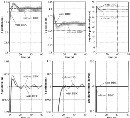
Table 2. Frequency response of the manipulator end-effector with and without DDC.
without DDC with DDC
base oscillation
frequency (Hz)
X amplitude
(mm)
Y amplitude
(mm)
X amplitude
(mm)
Y amplitude
(mm)
0.06 5.0 5.0 * *
0.1 6.0 6.0 * *
0.5 15 13 0.5 0.5
1 52 41 2.0 1.5
100 2.0 2.0 0.6 0.5
* down to simulated sensor resolution
0 20 40 60 0.8
0.85 0.9 0.95 1 1.05
time (s)
X
p
o
si
ti
o
n
(
m
)
0 20 40 60
0.8 0.85 0.9 0.95 1 1.05 1.1 1.15
time (s)
Y
p
o
si
ti
o
n
(
m
)
0 20 40 60
-10 0 10 20 30 40 50 60 70 80 90
time (s)
a
n
g
u
la
r
p
o
si
ti
o
n
(
d
e
g
r
e
e
s)
with DDC
without DDC
with DDC
without DDC
with DDC
without DDC
0 20 40 60
0.99 0.995 1 1.005 1.01
0 20 40 60 0 20 40 60
89.5 90 90.5
0.99 0.995 1 1.005 1.01
time (s)
X
p
o
si
ti
o
n
(
m
)
time (s)
Y
p
o
si
ti
o
n
(
m
)
time (s)
a
n
g
u
la
r
p
o
si
ti
o
n
(
d
e
g
r
ee
s)
with DDC
without DDC
with DDC
without DDC
with DDC
without DDC
Figure 13. Single system position control with and without dynamic disturbance compensation (DDC), for 0.5Hz (top) and 0.06Hz (bottom) base oscillations.
Copyright 2004 by ABCM July-September 2004, Vol. XXVI, No. 3 /267
0 10 20 30
0.5 1 1.5 2
X
p
o
si
ti
o
n
(
m
)
0 10 20 30
0 0.5 1
Y
p
o
si
ti
o
n
(
m
)
0 10 20 30
-40 -20 0 20
th
et
a
p
o
si
ti
o
n
(
d
eg
)
0 10 20 30
0 5 10 15 20
X
f
o
rc
e
(N
)
0 10 20 30
-5 0 5 10 15
Y
f
o
rc
e
(N
)
0 10 20 30
-10 -5 0 5 10
Z
t
o
rq
u
e
(N
-m
)
0 10 20 30
-1.5 -1 -0.5 0
X
p
o
si
ti
o
n
(
m
)
0 10 20 30
-0.5 0 0.5 1
Y
p
o
si
ti
o
n
(
m
)
0 10 20 30
140 160 180 200
th
et
a
p
o
si
ti
o
n
(
d
eg
)
0 10 20 30
-20 -15 -10 -5 0
X
f
o
rc
e
(N
)
Y
f
o
rc
e
(N
)
0 10 20 30
-10 -5 0 5 10
Z
t
o
rq
u
e
(
N
-m
)
Master robot endpoint position and force × time (s)
Slave robot endpoint position and force × time (s)
0 10 20 30
-5 0 5 10 15
Figure 15. Endpoint position and force of master robot (top) and slave robot (bottom).
0 0.5 1 1.5
0.8 0.85 0.9 0.95 1 1.05 1.1
time (s)
tr
u
ss
X
p
o
si
ti
o
n
(
m
)
0 0.5 1 1.5
0.7 0.75 0.8 0.85 0.9 0.95 1 1.05
time (s)
tr
u
ss
Y
p
o
si
ti
o
n
(
m
)
0 0.5 1 1.5
0 10 20 30 40 50 60 70 80 90
time (s)
tr
u
ss
a
n
g
le
(
d
eg
r
e
es
)
insertion completed
Figure 16. Truss segment position and orientation during insertion with dynamic disturbance compensation.
The second test involves two identical mobile robots (Table 1) cooperating using a model predictive master-slave hybrid position-force control architecture with surrogate sensing. In this task, the robots must insert a segment into a truss stage, which is slightly slanted by an angle of 6 degrees (which results in an insertion angle of 84 degrees). The manipulator bases are 2.5 m apart (in the horizontal direction), and the segment mass and inertia are respectively 2 kg and 0.21 kg⋅m2. Figure 14 shows 3D renderings of the simulation output at several stages during this insertion process.
Figure 15 shows simulation results of the endpoint positions and forces felt by the cooperating robots during the approach phase of the task. Although no external oscillation is forced on the base, there is significant base motion due to the interacting forces combined with the vehicle compliance. However, with predictive
Conclusions
This paper has addressed the problem of disturbance compensation for the successful assembly of structures by mobile field robots. A control architecture, consisting of a linear PID joint controller with model predictive feed-forward compensation for mobile base motions and interactive-force disturbance rejection has been discussed. Object insertion was achieved by predicting environment-object contact states using onboard force/torque sensors and inter-robot communication. Motions are planned in the direction of least resistance. Issues presented include dynamic modeling of multiple cooperative robots, control architecture design and stability analysis, and environment-object contact state prediction. Simulation results show the effectiveness of the control architecture.
References
Alur, R., 2000, “A Framework and Architecture for Multirobot Coordination”, Proceedings of the ISER 2000, Waikiki, Hawaii, USA.
Baumgartner, E.T., Schenker, P.S., Leger, C. and Huntsberger, T.L., 1998, “Sensor-Fused Navigation and Manipulation from a Planetary Rover”, Proceedings of the SPIE Symposium on Sensor Fusion and Decentralized Control in Robotic Systems, Vol. 3523, Boston, MA, USA.
Donald, B., Jennings, J. and Rus, D., 1997, “Information Invariants for Cooperating Autonomous Mobile Robots”, International Journal of Robotics Research, Vol.16, No. 5, pp. 673-702.
Gerkey, B. and Mataric, M.J., 2000, “Principled Communication for Dynamic Multi-Robot Task Allocation”, Proceeding of the ISER 2000, Waikiki, Hawaii, USA.
Giraud, A. and Sidobre, D., 1992, “A Heuristic Motion Planner using Contact for Assembly”, Proceedings of the 1992 IEEE International Conference on Robotics and Automation, Vol.3, Nice, France, pp. 2165-2170.
Hirai, S. and Iwata, K., 1992, “Recognition of Contact State Based on Geometric Model”, Proceedings of the 1992 IEEE International Conference on Robotics and Automation, Vol.2, Nice, France, pp. 1507-1512.
Huntsberger, T.L., 1997, “Autonomous Multi-Rover System for Complex Planetary Retrieval Operations”, Proceedings of the SPIE Symposium on Sensor Fusion and Decentralized Control in Autonomous Robotic Agents, Pittsburgh, PA, USA, pp. 220-229.
Kang, S., Kim, M., Lee, W.L. and Lee, K.-I., 1998, “A Target Approachable Force-Guided Control for Complex Assembly”, Proceedings of the 1998 IEEE International Conference on Robotics and Automation, Leuven, Belgium.
Khatib, O., 1995, “Force Strategies for Cooperative Tasks in Multiple Mobile Manipulation Systems”, Proceedings of the ISER 1995, Munich, Germany.
Kitagaki, K., Ogasawara, T. and Suehiro, T., 1993, “Methods to Detect Contact State by Force Sensing in an Edge Mating Task”, Proceedings of the 1993 IEEE International Conference on Robotics and Automation, Vol.2, Atlanta, GA, USA, pp. 701-706.
Kittipongpattana, T. and Laowattana, D., 1998, “Robotic Insertion of Dual Pegs based on Force Feedback Signals”, IEEE Proceedings of the Asia Pacific Conference on Circuits and Systems, pp. 527-530.
Lee, S. and Asada, H., 1999, “A Perturbation/Correlation Method for Force Guided Robot Assembly”, IEEE Transactions on Robotics and Automation, Vol.15, No. 4, pp. 764-773.
Marapane, S.B., Trivedi, M.M., Lassiter, N., Holder, M.B., 1996, “Motion Control of Cooperative Robotic Teams through Visual Observation and Fuzzy Logic Control”, Proceedings of the 1996 IEEE International Conference on Robotics and Automation, Vol.2, Minneapolis, MN, USA, pp. 1738-1743.
Mataric, M.J., 1998, “Coordination and Learning in Multi-Robot Systems”, IEEE Intelligent Systems, March/April 1998, pp. 6-8.
McCarragher, B.J. and Asada, H., 1993, “A Discrete Event Approach to the Control of Robotic Assembly Tasks”, Proceedings of the 1993 IEEE International Conference on Robotics and Automation, Atlanta, GA, USA.
Osborn, J.F., 1989, “Applications of Robotics in Hazardous Waste Management”, Proceedings of the SME 1989 World Conference on Robotics Research, Gaithersburg, MD, USA.
Parker, L.E., 1995, “The Effect of Action Recognition and Robot Awareness in Cooperative Robotic Teams”, Proceedings of the 1995 IEEE International Conference on Robotics and Automation, Vol.1, Nagoya, Japan, pp. 212-219.
Shaffer, G. and Stentz, A., 1992, “A Robotic System for Underground Coal Mining”, Proceedings of the 1992 IEEE International Conference on Robotics and Automation, Vol.1, pp. 633-638.
Shimokura, K. and Muto, S., 1996, “A High Speed Method of Detecting Contact-State Transitions and its Implementation in a Task-Coordinate Manipulation System”, Proceedings of the 1996 IEEE International Conference on Robotics and Automation, Minneapolis, MN, USA.
Sujan, V.A., 2002a, “Optimum Camera Placement by Robot Teams in Unstructured Field Environments”, Proceedings of the IEEE International Conference on Image Processing (ICIP), Rochester, NY, USA.
Sujan, V.A., 2002b, “Task Directed Imaging in Unstructured Environments by Cooperating Robots”, submitted to the 2002 Third Indian Conference on Computer Vision, Graphics and Image Processing, Ahmedabad, India.
Sujan, V.A. and Dubowsky, S., 2002, “Visually Built Task Models for Robot Teams in Unstructured Environments”, Proceedings of the 2002 IEEE International Conference on Robotics and Automation, Washington, D.C., USA.
Takanishi, A., Tochizawa, M., Karaki, H. and Kato, I., 1989, “Dynamic Biped Walking Stabilized With Optimal Trunk And Waist Motion”, Proceedings of the 1989 IEEE/RSJ International Workshop on Intelligent Robots and Systems (IROS’89) - The Autonomous Mobile Robots and Its Applications, pp. 187 –192.
Veloso, M. and Stone, P., 1999, “Task Decomposition and Dynamic Role Assignment for Real-Time Strategic Teamwork”, Intelligent Agents V – Proceedings of the International Workshop on Agent Theories, Architectures and Languages, Springer-Verlag, Heidelberg.