www.atmos-chem-phys.org/acp/6/433/ SRef-ID: 1680-7324/acp/2006-6-433 European Geosciences Union
Chemistry
and Physics
Boundary layer structure and decoupling from synoptic scale flow
during NAMBLEX
E. G. Norton1, G. Vaughan1, J. Methven2, H. Coe1, B. Brooks3, M. Gallagher1, and I. Longley1
1School of Earth, Atmospheric and Environmental science, University of Manchester, Building Sackville Street, Manchester,
M60 1QD, UK
2Department of Meteorology, University of Reading, P.O. Box 243, Earley Gate, Reading, RG6 6BB, UK 3School of the Environment, University of Leeds, Leeds, LSJ 9JT, UK
Received: 21 March 2005 – Published in Atmos. Chem. Phys. Discuss.: 23 May 2005 Revised: 2 November 2005 – Accepted: 2 November 2005 – Published: 8 February 2006
Abstract. This paper presents an overview of the meteo-rology and planetary boundary layer structure observed dur-ing the NAMBLEX field campaign to aid interpretation of the chemical and aerosol measurements. The campaign has been separated into five periods corresponding to the prevail-ing synoptic condition. Comparisons between meteorologi-cal measurements (UHF wind profiler, Doppler sodar, sonic aneometers mounted on a tower at varying heights and a standard anemometer) and the ECMWF analysis at 10 m and 1100 m identified days when the internal boundary layer was decoupled from the synoptic flow aloft. Generally the agree-ment was remarkably good apart from during period one and on a few days during period four when the diurnal swing in wind direction implies a sea/land breeze circulation near the surface. During these periods the origin of air sampled at Mace Head would not be accurately represented by back trajectories following the winds resolved in ECMWF analy-ses. The wind profiler observations give a detailed record of boundary layer structure including an indication of its depth, average wind speed and direction. Turbulence statistics have been used to assess the height to which the developing inter-nal boundary layer, caused by the increased surface drag at the coast, reaches the sampling location under a wide range of marine conditions. Sampling conducted below 10 m will be impacted by emission sources at the shoreline in all wind directions and tidal conditions, whereas sampling above 15 m is unlikely to be affected in any of the wind directions and tidal heights sampled during the experiment.
Correspondence to:E. G. Norton ([email protected])
1 Introduction
The North Atlantic Marine Boundary Layer EXperiment (NAMBLEX) took place during between 1 August and 1 September 2002 at the Mace Head atmospheric research sta-tion (53.32◦N, 9.90◦W) on the west coast of Ireland (Heard, 2005).
434 E. G. Norton et al.: Boundary layer structure during NAMBLEX
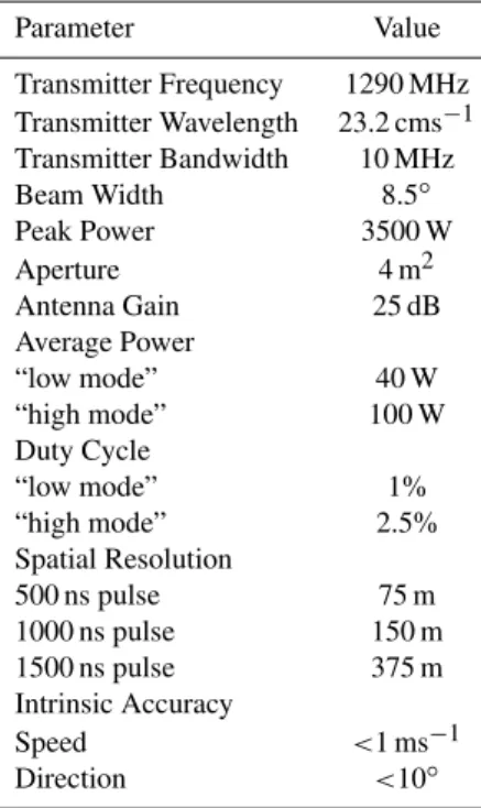
Table 1.Characteristics of the UFAM mobile 1290 MHz wind
pro-filer.
Parameter Value Transmitter Frequency 1290 MHz Transmitter Wavelength 23.2 cms−1 Transmitter Bandwidth 10 MHz Beam Width 8.5◦ Peak Power 3500 W Aperture 4 m2 Antenna Gain 25 dB Average Power
“low mode” 40 W “high mode” 100 W Duty Cycle
“low mode” 1% “high mode” 2.5% Spatial Resolution
500 ns pulse 75 m 1000 ns pulse 150 m 1500 ns pulse 375 m Intrinsic Accuracy
Speed <1 ms−1 Direction <10◦
This paper will first describe the specialist meteorologi-cal instrumentation used at Mace Head. We then present an overall meteorological summary of the NAMBLEX cam-paign, dividing it into five broad periods of similar synoptic type. Within each period, we present a time series of mea-surements from the various instruments and compare them to ECMWF analysis fields, to determine how well the analyses represented the local conditions. This in turn is a measure of the reliability of trajectory calculations based on ECMWF data. Subsequently, we concentrate on measurements of boundary-layer structure made by the UHF wind profiler, which show how representative the surface measurements were of the boundary layer as a whole. Finally turbulence statistics from the sonic anemometers are presented to asses the development of an internal layer.
2 Instrumentation
2.1 UHF wind profiler
“Clear-air” radars detect small scale irregularities in backscattered signals due to refractive index inhomo-geneities caused by turbulence C2n; (Doviak and Zrnic, 1993). In the lower troposphere such inhomogeneities are mainly produced by humidity fluctuations. “Clear-air” Doppler shifts provide a direct measurement of the mean radial ve-locity along the radar beam. UHF radars also observe strong
echoes from precipitation which can be distinguished from the “clear-air” echo by their intensity and spectral width.
The University Facility for Atmospheric Measurements (UFAM) mobile wind profiler is a “clear-air” UHF Doppler radar system designed by Degreane Horizon to measure three components of wind 24 h a day under all weather conditions. The radar operates at 1290 MHz (23 cm) with a peak power of 3.5 kW and beam width of 8.5◦. The radar consists of three panels that emit and receive three separate beams, each panel being an array of 64 dipole antennas. The vertical beam mea-sures the vertical component of the wind and the two beams at an elevation of 73◦and orthogonal azimuths sample radial velocities that have contributions from both vertical and hor-izontal wind components, to enable full wind vectors to be calculated. The radar provides measurements of wind speed and direction to an intrinsic accuracy of<1 ms−1and<10◦,
respectively, according to the manufacturer’s estimates. The radar was cycled between measurements in two modes: the “low mode” with a Gaussian shaped pulse of length 500 ns, inter-pulse period of 50µs, average power of 40 W and duty cycle of 1%; and the “high mode” with a rect-angularly shaped pulse of length 1000 ns, inter-pulse period of 40µs, average power of 100 W and duty cycle of 2.5%. The vertical resolution was 75 m for the “low mode” and 150 m for the “high mode” up to altitudes of approximately 1500 m and 4000 m, respectively, depending on atmospheric conditions. The minimum altitude was 75 m, although in practice it was found to be in the region of 200 m due to ground clutter echoes. The characteristics of the UFAM mo-bile wind profiler are summarized in Table 1.
Echoes from the three beams at each altitude were com-bined and both temporal and vertical windowing was used to distinguish the “clear-air” signal from any ground clutter or other interference. The wind profiler was located outside the top cottage 30 m above sea level and approximately 300 m from the shoreline. Measurements were derived every 15 min using consensus averaging over 30 min around the nominal observation time. The radar was operational 24 h a day un-der all weather conditions for the duration of the campaign apart from when a timing fault on the transmit-receive switch caused the limiter to fail. This resulted in no wind profiler data between the 15 and 21 August.
2.2 Surface layer flux measurements
Table 2.Scintec MFas64 technical specifications.
Number of Elements 64 Frequency Range 1650–2750 Hz Beam Angles 0◦,±22◦,±29◦ Number of frequencies Up to 80, (10 within
a single sequence) Number of vertical layers 100 Thickness of layer 10–250 m Maximum range 1000 m Minimum measurement height 20 m Intrinsic Accuracy
Horizontal speed 0.1–0.3 ms−1 Vertical speed 0.03–0.1 ms−1 Direction 2–3◦ Averaging time 1 min to 60 min
speeds in the u, v and w co-ordinates were recorded every 0.05 s, providing 10 Hz response and turbulence statistics as a function of height above the surface.
2.3 Sodar
The UFAM Doppler Sodar (SOnic Detection And Rang-ing) used during NAMBLEX was a Scintec MFAS64: a monostatic phased array system with 64 transmit and 64 receive transducers generating acoustic signals in the fre-quency range 1650 to 2750 Hz. The phased array allows for both the transmitted and the received signals to be steered and the effect of side lobe interference reduced. Table 2 gives the detailed technical specifications of the system.
In a monostatic sodar system only the backscattered signal is detected. The intensity of the returned energy is propor-tional to the C2T function, which, in turn, is related to the ther-mal structure and stability of the atmosphere. C2T has char-acteristic patterns during ground-based radiation inversions, within elevated inversion layers, at the periphery of convec-tive columns or thermals, in sea breeze/land breeze frontal boundaries, and at any interface between air masses of dif-ferent temperatures. The acoustic scattering is determined by Bragg scattering laws and only inhomogenities of the order of 1/2 the acoustic wavelength (5–10 cm) contribute. Using Doppler methods a measure of air movement at the position of the scattering eddy can be determined.
In this application ten frequencies were used (Table 3) with longer pulse lengths at the lower frequencies to increase mea-surement range and shorter pulses at higher frequencies to increase height resolution. The acoustic beam was steered around four reference directions in turn (N, E, S, W) with a pulse sequence as described in Table 3; alternate pulses were directed either side of the reference direction. The reason for the two low frequency short duration pulses at the end is so they don’t interfere with the rest of the sequence.
Table 3.Pulse sequence used during NAMBLEX.
Frequency (Hz) Pulse length (m) 2022.0 210 2124.8 150 2227.6 100 2330.4 80 2433.2 50 2536.1 40 2638.9 30 2741.7 20 1919.2 10 1713.6 10
The same pulse sequence was repeated 10 times for a given reference direction and the data averaged over 10 min. Due to the proximity of housing to the research site the operation of the sodar was restricted to the hours of 09:00 to 17:00 local time. During rain events the sodar output was reduced to zero due to scattering of the acoustic signal off the falling rain droplets.
3 Meteorological summary
This meteorological summary for the NAMBLEX period has been compiled from synoptic charts published by Weather for 12:00 GMT and the European Meteorological Bulletin for 00:00 GMT, along with meteorological measurements made at Mace Head. The daily maximum temperature over the campaign period remained in the range 12–17◦C except for a warm spell between 1 and 6 August when the tempera-ture was 16–20◦C, with a warm spike on the 2 August (up to 24◦C). Prevailing synoptic conditions were used to separate the campaign into five periods:
1. 1 August to 5 August was complex, with the Azores high extending over the Atlantic and a stagnant low pressure system over Ireland and the UK, with re-circulating fronts. Winds were very weak north-easterly from 1 to 5 August.
2. The Azores high extended towards Ireland and therefore winds were generally westerly or north-westerly from 6 to 11 August, apart from the 8th when the centre of a depression crossed just south of Mace Head.
3. From 12 to 17 August the Azores high retreated south allowing a succession of depressions to cross Ireland from the west.
436 E. G. Norton et al.: Boundary layer structure during NAMBLEX
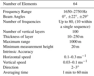
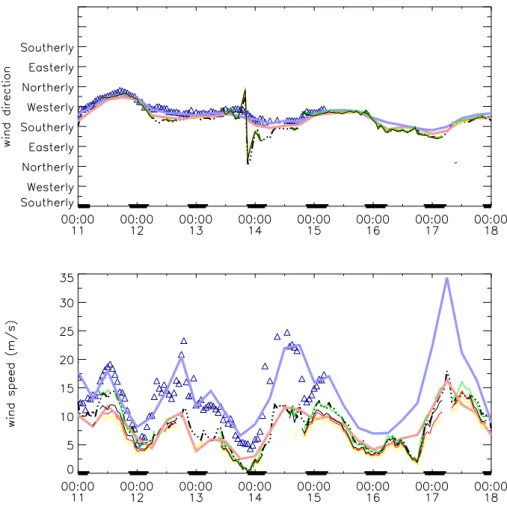
Fig. 1. Comparisons for period one between the ECMWF model analysis every 6 h at 10 m (pink line) and 1100 m (blue line) with mea-surements by sonic anemometers at 7 m (yellow line), 10 m (red line), 15 m (black line) and 24 m (green line), standard surface anemometer (black dashed line) and UHF wind profiler data (blue triangles) for(a)wind direction and(b)wind speed. The bold black line on the time axis indicates hours of darkness. On this plot for period one the lower and upper levels have been offset from one another for clarity. Note the close agreement in wind directions measured by the different anemometer make it is often difficult to distinguish between them.
5. The 28 to 31 August saw a return to westerlies and un-settled weather.
4 Comparison between wind speed and direction mea-surements and meteorological analysis.
In order to interpret the chemical measurements at Mace Head it is necessary to separate local and long-range contri-butions to the air sampled. This will be done by comparing the local wind measurements to those in the corresponding ECMWF analyses, and examining the consistency between surface winds and the flow aloft. The ECMWF analysis data used has a horizontal resolution T159 (grid spacing of about 1.125 degrees) and 60 levels in the vertical in terrain fol-lowing eta-coordinates. The lowest level is at approximately 10 m and the 11th is at about 1100 m. We present compar-isons of wind speed and direction for two altitude regions: at low level between the 7 m, 10 m, 15 m and 24 m sonic anemometers, a standard anemometer at 21 m and ECMWF
analyses at 10 m; and near the top of the boundary layer be-tween the wind profiler at 1100 m and ECMWF analyses at 1100 m. Sodar data at 100 m was also included in the com-parisons for periods four and five. In the plots that follow night-time is indicated as the bold black line on the time axis. 4.1 Meteorological period one
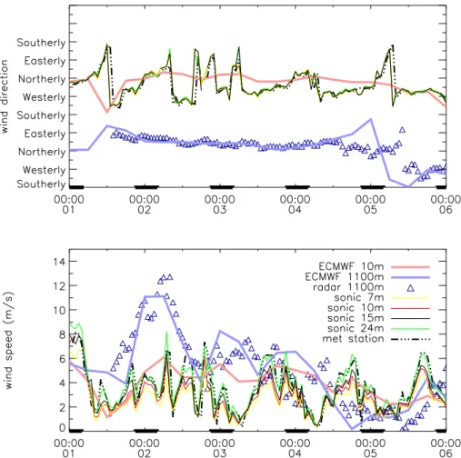
Fig. 2.The same as Fig. 1 but for period two.
The lower level winds were much more variable with a general tendency to be from the north-western quadrant. This variability was not represented in the ECMWF model winds which were generally northerly. During land breeze events the lower winds were measured to be more easterly. This is clear on the night of the 2nd, 4th and 5th when the wind direction switched to be more easterly than the model dur-ing the night. The opposite occurred a few hours after dawn when the direction shifted more westerly than the ECMWF model. This is a characteristic sea breeze pattern. Close agreement in the wind directions was observed between the sonics positioned at different heights on the tower. Period one was characterised by low wind speeds with a local cir-culation being the dominant influence on the ground based chemical measurements.
Comparisons between the wind speed values are also shown in Fig. 1. The radar and ECMWF analyses at 1100 m agree to within <2 ms−1 apart from the night of the 4th. At the lower levels wind speeds were very variable on 1st and 2nd, then settled into a sea breeze pattern with min-imum speeds in early morning and maxima in late after-noon. The sea breeze circulation was not represented in the ECMWF model which bears little resemblance to the
lower-level winds. These comparisons confirm that period one was dominated by local flow introducing a high degree of error to trajectory calculations based on the ECMWF model. Indeed there are occasions in Fig. 1 where the sonic anemometers at 10 m (red line) and 24 m (green line) on the tower show wind speeds that differ by up to to 2.0 ms−1, emphasizing that species at different altitudes during this period cannot be assumed to share a common source region.
4.2 Meteorological period two
This pattern of sea and land breezes disappeared on the morn-ing of 6 August after the passage of an occluded front. Hence period two was defined between 6 and 11 August. Dur-ing this period the wind direction was generally westerly to north-westerly, apart from the 8th when the centre of a de-pression passed just south of Mace Head. During the pas-sage of the depression the wind direction went full circle in an anti-clockwise direction from northwesterly to northerly.
438 E. G. Norton et al.: Boundary layer structure during NAMBLEX
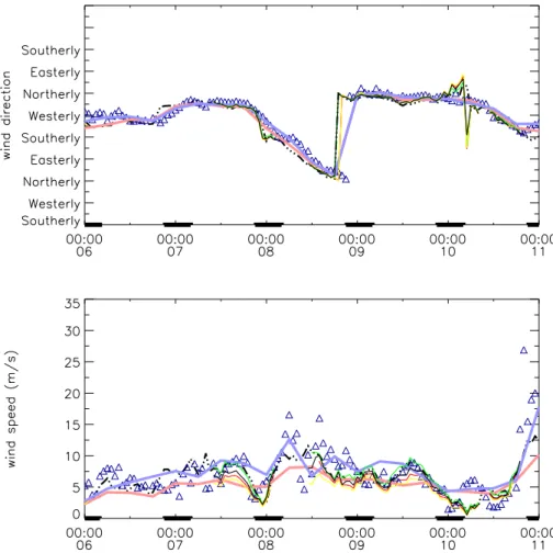
Fig. 3.The same as Fig. 1 but for period three.
a brief exception to this rule occurred on the night of the 10th when the wind speed dropped to <2 ms−1 and hence local circulation effects dominated. For most of this period the wind speeds at 1100 m were similar to those near the ground. Interestingly this agreement is not exhibited by the ECMWF analyses, where winds are almost always stronger at the higher level. The model also fails to capture the vari-ability of the measured winds, suggesting that some local in-fluences were present during this period. Nevertheless, the good agreement in wind direction and overall average cor-rectness of the speeds suggests that the ECMWF trajectory calculations should be fairly reliable during this period. 4.3 Meteorological period three
Another depression and occluded front passed over Mace Head on the evening of the 10th and early hours of the 11th. After the depression passed, a north-westerly airflow ensued and a ridge of high pressure started to develop, defining pe-riod three. During this pepe-riod three frontal systems passed over Mace Head, with the wind direction retaining a west-erly component throughout (Fig. 3). As in period two the measured wind directions at the upper and lower levels were
almost identical, with the ECMWF model in close agree-ment. An exception was observed during the night/morning of the 13th/14th when the lower level wind vector rotated through the west. This was accompanied by very low wind speeds<2 ms−1. This time however the model and
measure-ments also agree on wind speed (Fig. 3), with both showing winds approximately 5 ms−1stronger at the upper level than
the lower level. We therefore conclude that trajectory calcu-lations should be valid during this period.
4.4 Meteorological period four
After the passage of a warm and a cold front on the 17th the wind speed dropped off and anti-cyclonic conditions set in, with the direction remaining generally westerly (Fig. 4). Radar data were only available from the 22nd on and agree very well with the ECMWF model direction. The ECMWF analyses seem to capture a weak representation of the sea breeze from the 18th to 20th, seen in the low level wind di-rection and speed (Fig. 4). A sea breeze also occurred on the 25th.
Fig. 4.The same as Fig. 1 but for period four and including sodar data (red crosses).
measurements at 100 m (red crosses), available only during the day, closely tracked the ECMWF model at 10 m apart from the 23rd for speed. This was because in low wind con-ditions (<5 m/s) the sodar is more susceptible to the effects of ambient noise. This problem is reduced by using a 2 m high acoustic shield, unfortunately during this period only a 1 m hight shield was used. Agreement with the model wind speeds is generally good at both levels apart from the sea breeze events. Trajectory calculations, outside of the sea breeze periods, should be reliable during this period.
4.5 Meteorological period five
Radar data ceased on the 30th and the anemometers and so-dar data on 1 September as the campaign ended. This west-erly period was very similar to period two, with excellent agreement in wind direction between all the measurements and the ECMWF model and little directional wind shear in the boundary layer as shown by Fig. 5. At both levels the wind speeds showed good agreement as shown by Fig. 5 in-dicating that trajectory calculations should be reliable during this period.
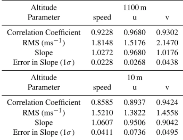
Table 4.Comparison statistics of the ECMWF model analysis with the wind profiler at 1100 m (1–15 and 21–31 August) and with the sonic anemometer at 10 m (6–19, 22–24 and 26–31 August) .
Altitude 1100 m Parameter speed u v Correlation Coefficient 0.9228 0.9680 0.9302
RMS (ms−1) 1.8148 1.5176 2.1470 Slope 1.0272 0.9680 1.0176 Error in Slope (1σ) 0.0228 0.0268 0.0438
Altitude 10 m Parameter speed u v Correlation Coefficient 0.8585 0.8937 0.9424
440 E. G. Norton et al.: Boundary layer structure during NAMBLEX
Fig. 5.The same as Fig. 4 but for period five.
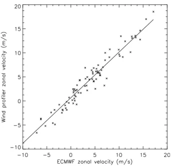
Fig. 6.Comparison of wind profiler and ECMWF zonal velocity of wind at 1100 m during NAMBLEX.
4.6 Comparison statistics
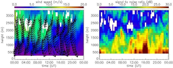
Fig. 7.1290 MHz wind profiler data for the 4 August 2002(a)Wind speed and direction(b)Minimum signal to noise ratio.
within 1 σ, showing that there is no detectable systematic offset between the model analyses and the measurements at either level outside of the sea breeze periods. Figure 6 shows an example of a scatter plot for the zonal component of wind for the wind profiler throughout the duration of the campaign.
5 Planetary boundary layer structure
The Planetary boundary layer (PBL) is defined as the low-est part of the atmosphere directly influenced by the Earth’s surface on a time period of 1 day or less (Stull, 1988). The depth of this layer is dependent on surface heating by the Sun leading to convection. Over land under high pressure condi-tions there is usually a daily cycle of the planetary bound-ary layer, growing during the day and collapsing at night as the Earth’s surface cools and mixing is suppressed. During the night (or over the ocean) a stable boundary layer often forms. Coupling between the PBL and the surface has an im-pact on understanding ground-based chemical measurements made during NAMBLEX. This section gives a brief overview of the PBL structure during NAMBLEX. The structure of the PBL at the coastal environment of Mace Head was ob-served by lidar during PARFORCE to vary from a single well mixed layer to multilayered structures (Kunz, 2002). The UHF radar observations during NAMBLEX showed that the PBL was more complex than at an inland location hence full details of the PBL structure during NAMBLEX will be given in a later paper.
Two properties of the atmosphere give rise to UHF radar echoes: turbulence and vertical gradient in refractive index. Where they occur together as in a convective plume strong echoes results, so that the radar can readily identify the con-vectively mixed boundary layer. In the lower atmosphere re-fractive index gradients are caused mainly by humidity gradi-ents, so the radar can identify the hydrolapse typically found
at the top of the boundary layer, as well as internal residual layers (Angevine et al., 1994; Angevine et al., 1998; Grims-dell and Angevine, 1998).
On sea breeze days such as 4 August a stable boundary layer with shear-driven turbulence was observed. On this day the prevailing wind was north-easterly (Fig. 7). The reflectiv-ity profiles show that in this case there is no obvious diurnal evolution of a mixed layer. Enhanced signals are sometimes observed up to altitudes as high as 2000 m but it is not clear where to assign the depth of the boundary layer. The en-hanced reflectivity at 16:00 was due to Rayleigh scattering from precipitation.
442 E. G. Norton et al.: Boundary layer structure during NAMBLEX
Fig. 8. The same as Fig. 7 but for the 9 August 2002. Note the clockwise turning of the wind direction with height within the turbulent boundary layer is extremely clear in this picture.
Fig. 9.The same as Fig. 7 but for the 11 August 2002.
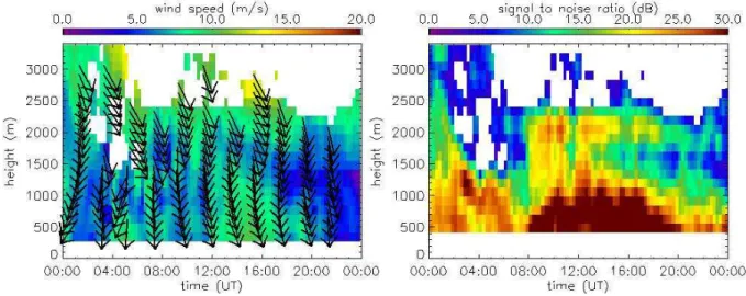
Updrafts during large scale weather features such as the passage of the occluded front on the afternoon of the 10 Au-gust obliterated any surface effects as shown in Fig. 10. PBL air is transported high into the atmosphere hence strong re-flectivity signals are observed to>3000 m. During the strong winds between 17:00 and 23:00 h the enhanced SNR was as-sociated with precipitation. During the passage of this weak forward-sloping (kata) front the wind speeds were observed to increase very suddenly by approximately 10 ms−1. There was no significant change in wind direction associated with the front shown in Fig. 10. The change in wind direction pre-ceding the front was associated with a ridge of high pressure passing over the site.
To summarise, the idealised convective land based diurnal cycle of the PBL was only observed on a few days. The more typical PBL during the NAMBLEX campaign was one
that was more oceanic in nature showing much less diurnal variation and less evidence for strong vertical mixing.
6 Surface layer turbulence structure
Z
,2x
1x
2x
3x
δ
Z
,1Z
Fig. 10.The same as Fig. 7 but for the 10 August 2002.
Z
0,2x
1x
2x
3x
δ
Z
0,1Z
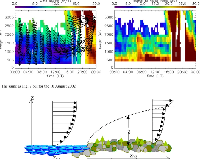
Fig. 11.Schematic of the development of an internal boundary layer arising from a change in surface roughness at the shoreline.
from the immediately underlying air. Wave breaking on the shoreline will produce large sea salt particles (Kunz, 2002) and this production is likely to be significantly influenced by the developing internal boundary layer and will be retained within it. The inter-tidal zone at Mace Head has previously been shown to be a source of iodocarbons (Carpenter, 2003) and these species have been linked with ultrafine particle for-mation (O’Dowd et al., 2002; McFiggans et al., 1998). The developing internal boundary layer will act to restrict the ver-tical diffusion of such emissions. It was therefore important to understand the micrometeorology of the internal bound-ary layer in a range of stability conditions, wind directions and tidal heights during NAMBLEX to establish whether the sample inlets were likely to be within the internal boundary layer and therefore whether they may be impacted by any gas or particle sources in the inter-tidal zone.
Turbulence statistics were calculated from the sonic data every 15 min throughout the experiment Fig. 12. The stress is measured by the covariance of the horizontal and vertical
444 E. G. Norton et al.: Boundary layer structure during NAMBLEX
u'w'(z)/u'w'(24)
0 1 2 3
z / m 0 5 10 15 20 25 30 low tide high tide
u'w'(z)/u'w'(24)
0 1 2 3
z / m 0 5 10 15 20 25 30 SW W NW
Fig. 12. Normalised stress profile, averaged over the entire experimental period as a function of(a)wind direction degrees and(b)tidal height.
the stress perturbation is larger at low tide due to the greater exposure of the inter-tidal coast, however, there is no indi-cation that the perturbation affects the wind profile at 24 m, demonstrating that in all wind directions and tidal conditions the measurements made from the 24 m are free from the im-mediate influence of the shore. It is likely that measurements made at, or below 10–12 m, will be significantly impacted by shoreline or inter-tidal emissions. Previous work (Car-penter, 2003) has provided evidence for iodocarbon profiles that support these findings. It is recommended that the dis-continuities in the surface profile arising from changes in sur-face roughness be considered when interpreting data at Mace Head that is likely to have significant coastal sources.
7 Conclusions
This paper has presented a meteorological overview of the NAMBLEX field campaign, for use in interpreting the chem-ical measurements. The comparative investigations found that on the whole the ECMWF model analysis at 10 m and 1100 m agreed well with the meteorological measurements, but on a number of days the local winds were very different to the synoptic flow. The greatest discrepancies were ob-served between the 1 and 6 August when the winds were light and sea breeze effects dominated. Sea breezes were also observed between 17 and 22 August and on the 25th. On days when the local flow was different from the synoptic, trajectory calculations based on the ECMWF model should be treated with caution. The UHF radar reflectivity profile have also been used to identify days when the boundary layer could be considered convectively mixed up to ∼1 km. In fact such days were rare: when on-shore winds prevailed the boundary layer showed little evidence of active mixing above∼700 m. Turbulence statistics have been used to as-sess the development of the internal boundary produced by
the change in roughness at the shoreline at the measurements location.
Stress profiles show that in all marine sectors sampled the stress profile is perturbed, indicating the influence of the in-ternal boundary layer, at the 10 m sample level and below. There is some evidence that this may reach 15 m in the north westerly sector, though the terrain and the laboratory may induce artifacts under these conditions. The increased inter-tidal fetch at low tide is measurable in the stress profile but does not show that the internal boundary layer propagates to 24 m, even at low tide. However, sampling at, or below, 15 m may be affected under low tide conditions.
Acknowledgements. The authors would like to thank D. Heard
and all their colleagues involved in NAMBLEX. Credit is also due to P. Currier and colleagues at Degreane for their help with the wind profiler. This work was supported by University Facility for Atmospheric Measurements (UFAM) and British Atmospheric Data Centre (BADC).
Edited by: D. Heard
References
Angevine, W. M., White, A. B., and Avery, S. K.: Boundary layer depth and entrainment zone characteriztion with a bound-ary layer profiler, Bound.-Layer Meteor., 68, 375–385, 1994. Angevine, W. M., Grimsdell, A. W., Warnock, J. M., Clark, W. L.,
and Delany, A. C.: Flatland boundary layer experiments, Bull. Amer. Meteor. Soc., 79, 419–431, 1998.
Carpenter, L. J., Liss, P. S., and Penkett, S. A.: Marine organohalo-gens in the atmosphere over the Atlantic and Southern Oceans, J. Geophys. Res., 108(D9), 4256, doi:10.1029/2002JD002769, 2003.
Grimsdell, A. W. and Angevine, W. A.: Convective boundary laer height measuremnts with wind profilers and comparison to cloud base, J. Atmos. and Oceanic. Tech., 15(6), 1331–1338, 1998. Heard, D., Read, K., Methven, J., et al.: The North Atlantic
Ma-rine Boundary Layer Experiment (NAMBLEX). Overview of the campaign held at Mace Head, Ireland, in summer 2002, Atmos. Chem. Phys. Discuss., 5, 12 177–12 254, 2005,
SRef-ID: 1680-7375/acpd/2005-5-12177.
Kunz, G. J., de Leeuw, G., Becker, E., and O’Dowd, C. D.: Li-dar observations of atmospheric bounLi-dary layer structure and sea spray aerosol plumes generation and transport at Mace Head, Ireland (PARFORCE experiment), J. Geophys. Res., 107(D19), 8106, doi:10.1029/2001JD001240, 2002.
McFiggans, G., Coe, H., Burgess, R., Allan, J., Cubison, M., Al-farra, M. R., Saunders, R., Saiz-Lopez, A., Plane, J. M. C., Wevill, D. J., Carpenter, L. J., Rickard, A. R., and Monks, P. S.: Direct evidence for coastal iodine particles from Laminaria macroalgae – linkage to emissions of molecular iodine, Atmos. Chem. Phys., 4, 701–713, 2004,
SRef-ID: 1680-7324/acp/2004-4-701.
O’Dowd, C. D., Jimenez, J. L., Bahreini, R., Flagan, R. C., Seinfeld, J. H., Hameri, K., Pirjola, L., Kulmala, M., Jennings, S. G., and Hoffmann, T.: Marine aerosol formation from biogenic iodine emissions Nature, 417(6889), 632–636, 2002.