Characterizing summertime chemical boundary conditions for
airmasses entering the US West Coast
G. G. Pfister1, D. D. Parrish2, H. Worden1, L. K. Emmons1, D. P. Edwards1, C. Wiedinmyer1, G. S. Diskin3, G. Huey4, S. J. Oltmans2, V. Thouret5,6, A. Weinheimer1, and A. Wisthaler7
1Atmospheric Chemistry Division, National Center for Atmospheric Research (NCAR), Boulder, CO, USA 2Earth System Research Laboratory, National Oceanic and Atmospheric Administration, Boulder, CO, USA 3Chemistry and Dynamics Branch, NASA Langley Research Center, Hampton, VA, USA
4School of Earth & Atmospheric Sciences, Georgia Institute of Technology, Atlanta, GA, USA 5Laboratoire d’A´erologie, Centre National de la Recherche Scientifique, Toulouse, France 6Universit´e de Toulouse, Toulouse, France
7Institute for Ion Physics & Applied Physics, University of Innsbruck, Innsbruck, Austria Received: 26 October 2010 – Published in Atmos. Chem. Phys. Discuss.: 25 November 2010 Revised: 2 February 2011 – Accepted: 7 February 2011 – Published: 25 February 2011
Abstract. The objective of this study is to analyze the pol-lution inflow into California during summertime and how it impacts surface air quality through combined analysis of a suite of observations and global and regional models. The focus is on the transpacific pollution transport investigated by the NASA Arctic Research of the Composition of the Troposphere from Aircraft and Satellites (ARCTAS) mis-sion in June 2008. Additional observations include satel-lite retrievals of carbon monoxide and ozone by the EOS Aura Tropospheric Emissions Spectrometer (TES), aircraft measurements from the MOZAIC program and ozoneson-des. We compare chemical boundary conditions (BC) from the MOZART-4 global model, which are commonly used in regional simulations, with measured concentrations to quan-tify both the accuracy of the model results and the variability in pollution inflow. Both observations and model reflect a large variability in pollution inflow on temporal and spatial scales, but the global model captures only about half of the observed free tropospheric variability. Model tracer contri-butions show a large contribution from Asian emissions in the inflow. Recirculation of local US pollution can impact chemical BC, emphasizing the importance of consistency be-tween the global model simulations used for BC and the regional model in terms of emissions, chemistry and trans-port. Aircraft measurements in the free troposphere over California show similar concentration ranges, variability and
Correspondence to:G. G. Pfister ([email protected])
source contributions as free tropospheric air masses over ocean, but caution has to be taken that local pollution aloft is not misinterpreted as inflow. A flight route specifically designed to sample boundary conditions during ARCTAS-CARB showed a prevalence of plumes transported from Asia and thus may not be fully representative for average inflow conditions. Sensitivity simulations with a regional model with altered BCs show that the temporal variability in the pollution inflow does impact modeled surface concentrations in California. We suggest that time and space varying chem-ical boundary conditions from global models provide useful input to regional models, but likely still lead to an underesti-mate of peak surface concentrations and the variability asso-ciated with long-range pollution transport.
1 Introduction
(O3) (Zhang et al., 2008) have confirmed the large dis-tances over which pollutants can be transported. Ziemke et al. (2006) demonstrated the potential of using satellite-derived columns of tropospheric ozone (O3) in tracking pol-lution events either regionally or globally. Using observa-tions at a mountaintop in the Azores, Val Martin et al. (2006) showed that North American emissions frequently impacted this remote site. Tracer correlations of CO and O3have been used to identify the photochemical O3enhancement in long-range pollution events (Parrish et al., 1993; Bertschi et al., 2004) and of odd nitrogen (NOy)and O3to study the export efficiency of anthropogenic emissions (Li et al., 2004; Stohl et al., 2002). However, the quantification of the impact of long-range pollution events on local air quality is challeng-ing.
Recent modeling experiments have attempted to charac-terize the contribution of long-range pollutant transport. Us-ing global model simulations, Fiore et al. (2009) suggest that for Northern Hemispheric surface O3the response to foreign emissions is largest in spring and late fall, and that responses to emission reductions of the traditional O3precursors from a single foreign source region are often 10% (maximum of 50%) of the responses to domestic emission reductions. Ja-cob et al. (1999) calculated that a tripling of Asian anthro-pogenic emissions could increase monthly mean surface O3 over the US by 1–6 ppbV. And the modeling study by Li et al. (2002) suggested that 20% of the violations in Europe of the 8-h European Council O3standard of 55 ppbV would not have occurred without the contribution from pollution trans-port from North America. The imtrans-portance of intercontinen-tal pollution transport was recognized in 1994 with the es-tablishment of the Task Force on Hemispheric Transport of Air Pollution (HTAP) by the Executive Body of the UNECE Convention on Long-Range Transboundary Air Pollution.
The methods applied for setting chemical BC in regional air quality models range from the use of a single background value for selected long-lived tracers, through the use of ide-alized or observed vertical profiles, to using time and space varying output from global CTMs. Tang et al. (2007) stud-ied the sensitivity of regional air quality model simulations for the US to various lateral and top boundary conditions by comparing regional model simulations driven with chemical BC from three different global models. They found differ-ences in the mean CO concentrations as large as 40 ppbv, and the effects of the BCs on CO were important throughout the troposphere, even near the surface. They further conclude that applying BCs without time variation may lead to a sig-nificant bias in the predicted variability. Huang et al. (2010) have continued this work with an examination of the same summertime period that we investigate here. They find that characterizing the vertical structure of the BCs is important in summertime air quality simulations for California.
In principle, observations would be preferred for provid-ing chemical BC, but in practice it is not possible to ob-tain measurements for the necessary species with the
spa-tial and temporal resolution required by air quality models. This leads to uncertainties in the chemical BC used (e.g., non-representativeness on temporal scales, spatial interpo-lation errors), which then affect the results of the regional model simulations. Global models can provide the BC for any needed species for a wide range of spatial and temporal scales, but there is uncertainty in the accuracy of the model results. Our goal in this study is to compare model-generated chemical BCs for the air entering the US West Coast with measured concentrations to quantify both the accuracy of the model results and the variability in pollution inflow, and to examine the sensitivity of the temporal and spatial variabil-ity in chemical BC on surface O3over California.
In this study we focus on the transpacific pollution trans-port investigated by the NASA Arctic Research of the Com-position of the Troposphere from Aircraft and Satellites (ARCTAS) mission. As part of ARCTAS, the California Air Resources Board (CARB) sponsored one week of flights over California and the eastern North Pacific in June 2008. The objectives were to provide measurements that help to improve state emission inventories for greenhouse gases and aerosols, and to test and improve models of ozone and aerosol pollution (Jacob et al., 2010). A boundary conditions flight was especially designed to capture the pollution inflow into California and to provide observational constraints on chemical BCs to be used in regional air quality models.
Here we examine the characteristics of air entering the US West Coast in regard to magnitude and variability based on ARCTAS-CARB and other measurements and evaluate how well the global Model for Ozone and Related Chemical Trac-ers (MOZART-4), which is frequently used for chemical BC in regional models, captures the observed characteristics. We limit our analysis to the three longer-lived gases CO, O3and peroxyacetyl nitrate (PAN), which likely are transported at sufficient concentrations to affect downwind photochemistry. The outline of the paper is as follows. In Sect. 2 we intro-duce the aircraft and satellite observations together with the modeling tools. In Sect. 3 we evaluate the global model for its representativeness of chemical inflow based on compari-son to aircraft and satellite measurement, relate observations taken during the ARCTAS-CARB boundary conditions flight to the larger temporal and spatial scales and examine the rep-resentativeness of free tropospheric observations over land for pollution inflow. Section 4 presents a sensitivity study to demonstrate the importance of temporal and spatial consid-eration of chemical BC in a regional air quality simulation. The findings are summarized in Sect. 5.
2 Observational data sets and models
2.1 In-situ data
pling and an overall uncertainty of about 5%. CO measure-ments are derived from a diode laser spectrometer (Diskin et al., 2002; Sachse et al., 1987) with the uncertainty given as 2% or 2 ppbV. PAN measurements were conducted using a chemical ionization mass spectrometer (Slusher et al., 2004). The detection limit for PAN measurements is estimated as 7 pptV for a 1-s integration period with an estimated error bar of 15%.
In addition to ARCTAS-CARB aircraft data we make use of data from the MOZAIC (Measurement of OZone, wa-ter vapor, carbon monoxide and nitrogen oxides by Airbus In-service airCraft) program (Marenco et al., 1998; http: //mozaic.aero.obs-mip.fr). This program was initiated in 1993 by European scientists, aircraft manufacturers and air-lines and provides measurements of reactive gases on several commercial aircraft. CO measurements are made with an improved infrared correlation instrument with a precision of ±5 ppbv or ±5% for a 30-s averaging time (N´ed´elec et al., 2003). O3 is measured via dual beam UV absorption tech-nique with an uncertainty of ±2 ppbv or ±2% (Thouret et al., 1998). MOZAIC collects data along the flight corridors as well as vertical profiles over a large number of airports. In this study we use CO and O3 measurements taken dur-ing ascents and descents over the Los Angeles and Portland airports.
In addition we include ozone profiles measured on son-des launched from Trinidad Head (Oltmans et al., 2008). Trinidad Head is located along the northern coast of Cali-fornia and, because of its relatively remote coastal location (insignificant anthropogenic influences and prevailing mar-itime airflow), provides an opportunity to observe and mon-itor both regional and global influences. Ozone is measured using electrochemical sensors. Consistent procedures have been used throughout the 10-year measurement period that began in August 1997 (Johnson et al., 2002). Estimated precision of tropospheric profiles is ±5%. Most observa-tions are done on a weekly schedule with some frequency increased to daily during field campaigns.
2.2 TES satellite data
We utilize co-located nadir retrievals of CO and O3vertical profiles (Version ID F05 07) from the Tropospheric Emis-sions Spectrometer (TES), which was launched in July 2004 onboard the NASA EOS Aura satellite in a sun-synchronous orbit (about 1:30 p.m. local mean solar time ascending node). TES is an infrared Fourier transform spectrometer (Beer, 2006) with a ground footprint of each nadir obser-vation of about 5 km×8 km. We include data from both the nominal operation mode (global survey mode) and from special observations (step-and-stare mode). The sampling for the global survey mode is one observation every 160 km
tude.
TES profile concentrations, averaging kernels and error covariances are given for 67 pressure levels located mainly in the troposphere and lower stratosphere. TES CO and O3 profile observations typically have 1 to 2 pieces of informa-tion in the troposphere (Rinsland et al., 2006; Jourdain et al., 2007). Both TES CO and ozone profile retrievals have been compared against a variety of aircraft, in-situ, and model studies. The comparison to ozonesonde data (Nassar et al., 2008; Osterman et al., 2008; Worden et al., 2007) and lidar measurements (Richards et al., 2008) shows that TES O3is biased high by 3–10 ppbV, particularly in the upper tropo-sphere. TES CO profiles are within 15% of aircraft profiles (Luo et al., 2007; Lopez et al., 2008).
2.3 Chemistry transport modeling
The global model used in this study is the Model for Ozone and Related Chemical Tracers MOZART-4, which is described and evaluated in greater detail in Emmons et al. (2010a). It includes a comprehensive chemistry scheme with bulk aerosols for simulating tropospheric ozone and pre-cursors in remote and polluted environments. The simulation includes online calculations of photolysis rates, dry depo-sition, H2O, and biogenic emissions (Pfister et al., 2008a). MOZART output is frequently used for boundary conditions in regional chemical transport models (e.g. Tang et al., 2007; Fast et al., 2009; Mena-Carrasco et al., 2009; Lin et al., 2010).
For this study, MOZART-4 was driven by meteorologi-cal fields from NCEP (National Centers for Environmental Prediction) –Global Forecasting System (GFS) analyses at a horizontal resolution of∼0.7◦ by 0.7◦. The vertical res-olution of the model consists of 64 hybrid levels between the surface and 2 hPa (∼45 km). Instantaneous model fields were output every three hours. A number of synthetic model tracers are included in the simulations. These include CO tracers for two different source types, fossil fuel and bio-fuel sources (FF) and biomass burning sources (BB) for each of the following six regions: contiguous US (US), Alaska and Canada (AkCan), Asia (Asia), Europe and North Africa (EurAf), and Central America (Cam). In addition we track the ozone produced from NOxfire emissions within the con-tiguous US The tagging schemes are described in detail by Lamarque et al. (2005), Pfister et al. (2006) and Hess and Lamarque (2007).
and physics scheme. WRF-Chem includes online biogenic emissions and dry deposition and a photolysis scheme that is coupled with hydrometeors as well as aerosols. We run WRF-Chem with the MOZART chemical scheme, i.e. the same gas-phase chemistry as used in the global simulations, which is linked to the Goddard Chemistry Aerosol Radia-tion and Transport (GOCART) bulk aerosol scheme (Chin et al., 2002). This configuration has recently been released in WRF-Chem V3.2. The regional domain has a spatial resolu-tion of 12 km×12 km centered over California with 27 ver-tical levels between the surface and 50 hPa. Meteorological initial and boundary conditions are taken from the NCEP Eta North American Mescoscale (NAM) Analysis with analysis nudging for wind, temperature and humidity applied. Spa-tially and temporally varying chemical boundary conditions are provided by the MOZART simulation. WRF-Chem is setup to run with the Mellor-Yamada-Janjic boundary layer (Janjic, 2002) scheme and the Noah land surface model (Ek et al., 2003).
Global and regional models are based on the same emis-sion inventories where applicable. Anthropogenic emisemis-sions are based upon the US EPA’s 2005 National Emissions In-ventory (version 3) and over California are replaced by an emission inventory provided by the California Air Resources Board (Jeremy Avis, personal communication). Daily fire emissions have been provided by the Fire INventory from NCAR (FINN Version 1) (Wiedinmyer et al., 2006, 2010). Emissions in MOZART vary daily and in WRF-Chem hourly with the diurnal profile following recommendations by the Western Regional Air Partnership (WRAP; Report to Project No. 178-6, July 2005). Fire emissions in MOZART are re-leased at the lowest model level, while in WRF-Chem the online plume rise module (Freitas et al., 2007) is applied to distribute the fire emissions vertically. Biogenic emissions in both models are calculated online following the Model of Emissions of Gases and Aerosols from Nature (MEGAN) (Guenther et al., 2006). Emissions in the MOZART model for the rest of the globe are based on the ARCTAS emis-sion inventory developed by D. Streets and Qiang Zhang (http:/www.cgrer.uiow.edu/arctas/emissions.html).
3 Discussion
3.1 Chemical BC from ARCTAS-CARB flight over ocean and model results
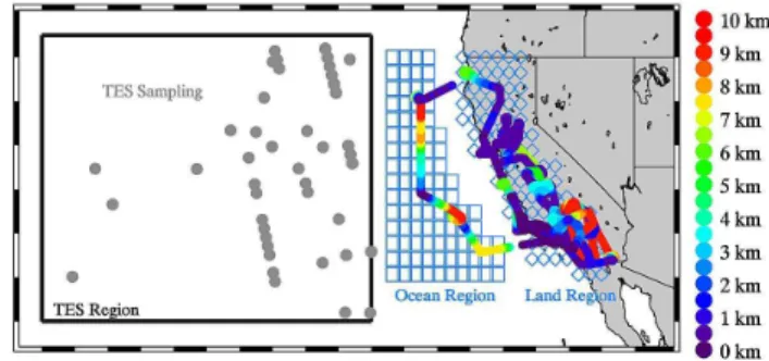
One of the scientific objectives of the NASA ARCTAS-CARB campaign was to investigate the pollution inflow into California from the Pacific, and to characterize the chemical boundary conditions suitable for California regional model-ing. For this purpose, one of the science flights (22 June) was designed to include a flight leg off the California coast with extensive vertical sampling and extending over the latitude range from Southern to Northern CA (Fig. 1). The
remain-Fig. 1. Locations of observational data sets and modeling regions:
Flight tracks of the boundary layer segment on 22 June 2008 and the flights over California are color coded by altitude. The ocean and land region over which additional model statistics (AVGRegion and AVGRegionTime) are performed are indicated by blue squares and blue diamonds, respectively. The TES sampling locations are shown by grey circles and the TES region is outlined by the black box.
der of the flight on 22 June and the other three science flights on 18, 20, and 24 June were performed mostly over land. In this section we perform a statistical analysis of the air-craft measurements over ocean of the longer lived chemical tracers (CO, O3, PAN), investigate the air mass characteris-tics in the free troposphere over ocean, and further examine how well the global model represents the observed statistics. Using the model as a reference, we examine the representa-tiveness of the flight sampling in the context of larger regions and longer time periods.
3.1.1 Measured and modeled concentrations
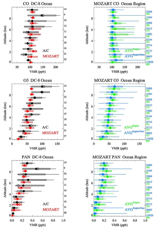
Fig. 2.Observed (black) and modeled (red) statistics for CO, O3and PAN vertical profiles along the DC-8 flight track (left-hand side) and for larger temporal and spatial averages (right-hand side; AVGRegion in green and AVGRegionTime in blue; see text and Fig. 1 for more explanation). Shown are mean (filled symbol), median (open symbols), 10th and 90th percentiles (bars) and extremes (lines). The number of data points per 1-km wide altitude bin is shown next to the graphs.
Overall, the model results interpolated to the flight track reproduce the magnitudes and mean profile shapes of mea-sured CO, O3, and PAN concentrations, but show less vari-ability with smaller extreme values, and overall lower con-centrations above 8 km. Both observation and model show
Fig. 3. Observed and modeled O3-CO and O3- PAN relationships for the aircraft path and respective larger regions. Aircraft data are color-coded by altitude as shown in legend. Larger region data (AVGRegionTime) are in black and gray with lighter shades indicating free tropospheric data (altitudes between 2–8 km). For illustration purposes, a 2-sided linear regression line to the flight track data is added to the graphs. The thin line in the MOZART plots (right-hand side) is a repeat of the fit to the aircraft observations.
plumes than captured in the model results along the flight track. Back trajectories for these flight segments (provided by H. Fuelberg; http://fuelberg.met.fsu.edu/research/arctas/ traj/traj.html) indicate that these plumes are related to long-range transport of pollution from Asia. At the highest alti-tude level, low observed CO and PAN and high O3indicates stratospheric influence. While the model simulates the aver-age PAN and CO concentrations at the highest altitude level well, it significantly underestimates O3suggesting a low bias in modeled stratospheric O3.
The spatial average (AVGRegion, green symbols in Fig. 2) shows enhanced concentrations and variability compared to the modeled flight track concentrations, especially in the middle troposphere around 4–7 km. This indicates that the model does capture concentrated pollution plumes, but that they are placed at lower altitudes compared to the measure-ments. Despite the larger sample size, the AVGRegion statis-tics do not reach the maximum range of the observed
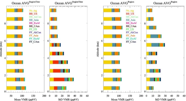
Fig. 4. Modeled CO Tracer concentrations (Mean and STD (ppbV)) for different CO Source types and temporal averages. Results for AVGRegionTime (left-hand side) and AVGRegion (right-hand side). (BB=Biomass burning; FF=Fossil Fuel). The contributions in (%) per 1 km high altitude bin and tracer type are given as numbers above each bar. See Table 1 for a summary of 2–8 km contributions.
3.1.2 Measured and modeled species relationships
While direct quantitative comparisons of individual species are crucial for evaluating the capability of a model to re-produce observed concentrations with regard to the magni-tude, vertical distribution and variability, it is also essential to evaluate the model fields in terms of accurately represent-ing relationships between different species. For this purpose we examine the data as scatter plots showing the relation-ships for CO-O3 and PAN-O3 (Fig. 3). The observed and modeled flight track concentrations as well as AVGRegionTime results (gray and black points) are shown. The model re-produces observed correlations well for the low and mod-erate concentration ranges where the bulk of the data is lo-cated. This is also demonstrated by the comparison of the two-sided linear fits calculated for the observed and modeled flight points. However, the model fails to reproduce relation-ships of high O3, CO and PAN concentrations at altitudes of about 7–10 km, which, as mentioned earlier, is likely linked to pollution from Asia.. The strong O3enhancements may be related to ozone production during the long-range transport of pollution plumes with different degrees of mixing with stratospheric air. Steep O3gradients at high altitudes are gen-erally an indication of stratospheric influence.
Not only the model results interpolated to the flight track, but also the larger model sample AVGRegionTimeare missing the representation of these observed correlations of substan-tial CO and PAN enhancements with varying O3 enhance-ments. A number of factors might be responsible for this
missing representation: uncertainty in the magnitude and emission ratios in the Asian inventory, missing representa-tion of direct injecrepresenta-tion of fire emissions into the free tro-posphere, model transport errors, insufficient mixing with stratospheric air, and/or too little O3 produced from light-ning generated NOx. Also the coarse spatial resolution of the model likely has an impact. Even though the grid resolu-tion of 0.7 degrees×0.7 degrees used here is fairly high for a global model, it still causes the model to overpredict chem-ical and physchem-ical dilution. Rastigejev et al. (2010) found that Eulerian chemical transport models (CTMs) have difficulty reproducing the layered structures of synoptic-scale pollu-tion plumes in the free troposphere due to numerical plume dissipation and conclude that proper simulation of such a plume would require an impractical increase in grid resolu-tion.
Table 1. Average CO Source Contributions for different CO tracers for AVGRegionTimeOcean data selections (entire data set; entire data set but with fire influenced data omitted; entire data set but selected for wind directions towards the continent) and the TES region for the 2–8 km altitude range. The latter is discussed in Sect. 3.3.1. Units are ppbV CO.
Ocean ALL Ocean noFire Ocean ALL TES Region WindDir 200–340 deg (130–150 W, 30–43 N)
NoTag 66.2±4.3 66.0±4.1 66.5±4.0 66.8±5.1 BB US 1.3±7.0 0.3±0.5 0.4±1.9 0.4±2.6 BB AKCan 0.0±0.0 0.0±0.0 0.0±0.0 0.0±0.0 BB Asia 10.6±3.3 10.5±3.3 10.6±3.5 12.7±5.0 BB EuAf 0.8±0.1 0.8±0.1 0.9±0.1 0.8±0.1 BB Cam 1.7±2.0 1.7±2.0 1.8±2.0 1.2±0.4 FF US 2.2±1.6 2.0±1.0 2.0±1.1 2.3±1.2 FF AKCan 0.2±0.1 0.2±0.1 0.2±0.1 0.2±0.1 FF Asia 17.0±4.2 17.0±4.3 16.8±4.4 18.4±4.8 FF EuAf 2.9±0.9 2.9±0.9 2.9±0.9 3.3±1.2 FF Cam 0.9±1.0 0.9±1.0 1.0±1.1 0.6±0.2
3.1.3 Model tagged species
To understand the origin of air masses carrying pollution plumes and to explore further the representativeness of the 22 June flight, we examine the source contributions using the model CO tracers for the 2-week period (AVGRegionTime)and for the day of the flight (AVGRegion)over the selected Ocean region. While the model shows an underrepresentation of high CO events, the comparison with the flight data in Fig. 2 as well as model evaluation results from previous studies (Pfister et al., 2008b, 2009; Emmons et al., 2010a, b) give confidence in the overall model performance for CO emis-sions, transport and distribution. Source contributions are analyzed by sampling model CO tracers for AVGRegionTime and AVGRegionselections (Fig. 4). The term “No tag” refers to the difference between the total CO and the sum of the individual CO tracers and is mostly due to CO produced from the photochemical oxidation of methane and other or-ganic species in the atmosphere, with a smaller contribution from untagged sources (Southern Hemisphere, biogenic and oceanic sources, aircraft emissions). The “No-tag” back-ground accounts on average for more than 50% of the total CO, which is in the range found in previous CO budget stud-ies (Granier et al., 1999; Horowitz et al., 2003; Pfister et al., 2004).
The AVGRegionTime results show large contributions throughout all altitudes from BB and FF sources in Asia. FF Asian contributions tend to be larger at the higher alti-tudes, which is also the altitude range where Asian plumes were sampled on the June 22 flight (Figs. 2 and 3) whereas the Asian BB tracer peaks at lower altitudes. Analysis of the model tracer transport (not shown here) shows that for the FF Asian tracer, with sources mostly south of about 40N, the transport pathways are at more southern latitudes and higher altitudes, while most BB sources in Asia at this time
of the year originate in northern Asia and those emissions are generally transported at higher latitudes and lower alti-tudes. We also see that US sources contribute to CO off the coast. The largest average contributions are seen at lower al-titudes with FF US. Large contributions also come from the US fires (in the AVGRegionTime, but not AVGRegion results). The US sources also add to the free tropospheric (>2 km) CO. The influence of fresh fire plumes is most pronounced at altitudes above 1 km and below about 4 km indicating that these plumes are transported at low altitudes but are not ef-ficiently mixed into the marine boundary layer over the dis-tances and time scales considered here.
The combined variability of CO in AVGRegionTime(as ex-pressed by the standard deviation) is up to about 40 ppbV (∼30%) at the lower altitudes decreasing to about 11 ppbV in the upper troposphere. A large part of the variability is driven by the US BB tracer, which dominates AVGRegionTime variability at the lower altitudes and contributes significantly through the mid-troposphere. Significant contributions also come from the Asian BB tracer and the Asian FF tracer. “No-tag/Photochemical” CO accounts for the major part of to-tal CO, but in comparison has a relatively small variability. Comparing AVGRegion to AVGRegionTime at the higher alti-tude levels, we find an increased contribution and variability of Asian transport on the flight day compared to the tempo-ral average, indicating that the flight day had an increased prevalence of plumes transported from Asia. We further find that the US BB tracer did not influence the selected region on the flight day, while the US FF influence on the flight day is comparable to the long-term sampling.
US. We only include observations with measured acetonitrile <0.25 ppbV and model results when the relative contribu-tions of the CO US fire tracers to total CO and of the O3US Fire Tracer to total O3are less than 5%. Fire influence was negligible in the flight track model results and in AVGRegion, but not in AVGRegionTime. Table 1 gives a summary of the free tropospheric source contributions and compares results with and without fire influence (filtering for fire influence reduces the number of points by about 5%). Omitting results with US BB has only a small influence on the contributions from tracers other than the US BB tracer. US FF slightly decreases reflecting the mixed outflow of FF and BB pollution.
We also include the average source contributions when model results are considered only with a wind direction di-rected towards the continent to select only airmasses being transported towards the US. In this case, the average con-tribution of US BB is clearly lower, but still has a non-negligible associated variability. This indicates that fresh fire plumes can be transported to the west off the coast followed by return to the continent. The US FF tracer changes little under this wind selection, which indicates that only a part of the US FF contribution to the boundary conditions is due to a direct recirculation of pollution. The CO lifetime is sev-eral weeks so it can be transported hemispherically, with US FF emissions entering the western boundary after “around-the-world” transport. Analysis of the spatial distributions of the model tracers (not shown here) support these transport patterns.
The results demonstrate that in choosing chemical bound-ary conditions for regional models the contributions from within the regional domain must be carefully considered. It should be noted that the fires in California started after 20 June so only parts of the considered time window po-tentially could have been impacted. Farther into an intense fire season, the fire emissions might have an even stronger influence. The results discussed here suggest that pollu-tion from within the US can contribute to the “chemical in-flow”, both through direct recirculation of west coast emis-sions transported offshore and, at least for long-lived tracers, also through “around-the-world” transport. To capture these effects, it is important to ensure the highest possible con-sistency in emissions, transport and chemistry between the global and the regional model. Additionally, extending the domain of the regional model as far off the coast as possible will improve the model performance. The US contribution must also be considered when analyzing and designing ob-servations for studying the chemical boundary conditions.
3.1.4 Free tropospheric statistics
We now evaluate how well the model reproduces the range and distribution of observed CO and O3values, the low end
spheric transport. This also allows for a more direct com-parison with TES retrievals (Sect. 3.3.1), which have low sensitivity near the surface, and with aircraft data over land (Sect. 3.2 and 3.3.2), which, especially at lower altitudes, might be influenced by local sources. Related percentiles for data sets with and without fire influence are specified in Ta-ble 2.
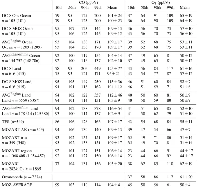
The model generally predicts a larger number of low to moderate CO values but underestimates the upper limit and overestimates the lower limit of the CO distribution. Assum-ing the 10th percentile as representative for CO background concentrations, then the model overestimates the observed background of 79 ppbV by about 15 ppbV. Omitting the fire influence in the AVGRegionTimemodel results has little effect on the lower end of the distribution, but reduces the high end. However, also in this case the model underestimates the ob-served tail (Table 2). The low model bias for the 99th per-centile is more pronounced compared to the 90th perper-centile, which is an indicator for the even stronger dilution of intense pollution plume events in the model.
The model also predicts a much narrower range of CO concentrations than observed. The 10th to 90th percentiles of the observations (no fire) span a range of 46 ppbV, while the model results along the flight track span a range of 27 ppbV. The corresponding ranges for AVGRegionand AVGRegionTime (no fire) are 37 ppbV and 24 ppbV, respectively; i.e. the model represents about half of the observed range of CO concentrations. Similar conclusions are reached if the 1– 99% range is considered (only 99th percentile is listed in Ta-ble 2). Overall the model results are biased high in CO com-pared to the observations. The mean observed concentration is 100±23 ppbV compared to 109±12 ppbV for the model flight track model results, 109±17 ppbV for AVGRegionand 102±10 ppbV for AVGRegionTime. The higher upper per-centiles, mean and standard deviation for AVGRegion com-pared to AVGRegionTimeagain support the finding that the 22 June flight day had a higher than average influence of pol-lution transport. The mean difference between the modeled and the observed flight data is 9±20 ppbV (12±16%).
With regard to the O3 distribution, the model does un-derestimate the high end as well as median of the observed O3 distribution, while being biased high on the low end. The range of O3(no fire) values spanned by the 10th–90th percentiles is 54 ppbV in the observations and 25 ppbV in the corresponding model results. The range for AVGRegion model results is 29 ppbV and for AVGRegionTime 28 ppbV. Similar to CO, the model reflects about half of the observed O3range.
Table 2. Percentiles, mean and standard deviation for different data sets (2–8 km or 850–350 hPa). The second row, where given, gives results when US fire influenced data are omitted. The numbers in the furthest left column give the number of data points that went into the no-fire impacted statistics if filtering was applied.
CO (ppbV) O3(ppbV)
10th 50th 90th 99th Mean 10th 50th 90th 99th Mean
DC-8 Obs Ocean 79 95 127 200 101±24 37 64 91 109 65±19 n=105(101) 79 95 125 200 100±23 36 64 90 109 64±19 DC-8 MOZ Ocean 95 107 123 144 109±13 46 56 70 73 57±10 n=105(101) 95 106 122 145 109±12 45 56 70 73 56±10
AVGRegionOcean 93 104 130 171 109±17 39 52 68 75 53±11
Oceann=1209(1209) 93 104 130 170 109±17 39 52 68 75 53±11
AVGRegionTimeOcean 92 100 119 154 104±14 37 49 65 81 50±12
n=154 752(148 706) 92 100 116 137 102±10 37 49 65 81 50±12 DC-8 Land 78 98 206 449 125±77 43 56 84 117 61±16 n=616(415) 75 93 121 171 95±21 43 54 77 87 57±12 DC-8 MOZ Land 95 105 149 250 115±36 46 51 60 84 52±7 n=616(415) 94 101 116 162 104±12 46 51 59 71 51±6
AVGRegionLand 94 102 122 357 112±46 40 50 60 81 50±9
Landn=5559(5057) 94 101 114 131 103±9 40 50 59 80 50±9
AVGRegionTimeLand 94 102 138 378 116±54 41 51 65 85 52±10
Landn=178 314(149 580) 93 100 114 137 102±9 41 50 62 79 51±10 TES (n=549) 86 106 128 163 107±17 43 54 68 84 55±11 MOZART AK (n=549) 94 106 130 140 109±13 39 47 54 66 47±7 MOZART true 93 102 137 151 109±17 35 49 71 80 51±14 n=549(548) 93 102 138 151 109±17 35 49 70 81 51±14 MOZART region 92 101 127 151 106±14 23 44 66 91 44±17 n=1 068 408(1 054 457) 92 101 127 150 106±14 23 44 66 92 44±17 MOZAIC 77 104 131 156 105±20 38 62 85 110 62±19 n=2824; O3n=1865
Ozonesonde (n=7374) 37 58 86 117 61±20 MOZ AVERAGE 99 103 110 114 104±4 45 50 56 61 50±4
model underestimates O3. The mean observed O3 concentra-tion is 64±19 ppbV compared to 56±10 ppbV for the mod-eled flight track model results, 53±11 for AVGRegion and 50±12 ppbV for AVGRegionTime. AVGRegionis again some-what enhanced over AVGRegionTime. The average difference for modeled and observed flight track data is –8±18 ppbV (–5±33%).
3.1.5 Statistics for boundary layer air
Marine boundary layer air (MBL) influences the surface air over California (Parrish et al., 2010), and for this reason we present an analysis of the 0–1 km altitude range for the above data sets. Table 3 lists percentiles of CO and O3
concentrations and Table 4 and Fig. 4 gives the average source contributions based on model CO tracers. Compared to the free troposphere, the tagged source analysis in the boundary layer indicates a somewhat higher contribution of no-tag/photochemical CO and enhanced contribution of BB Asia and slightly reduced contribution of FF Asia. The latter is in relation to the transport altitudes of Asian tracers dis-cussed in Sect. 3.3.1.
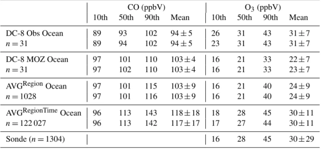
CO (ppbV) O3(ppbV) 10th 50th 90th Mean 10th 50th 90th Mean
DC-8 Obs Ocean 89 93 102 94±5 26 31 43 31±7 n=31 89 94 102 94±5 23 31 43 31±7 DC-8 MOZ Ocean 97 101 110 103±4 16 21 33 22±7 n=31 97 102 110 103±4 16 21 33 23±7
AVGRegionOcean 97 101 115 103±9 16 21 40 24±9
n=1028 97 101 116 103±9 16 21 40 24±9 AVGRegionTimeOcean 96 113 143 118±18 18 28 45 30±11 n=122 027 96 113 142 117±17 17 27 44 30±11 Sonde (n=1304) 16 28 45 30±29
Table 4. Average CO Source Contributions for AVGRegionTime
Ocean and the 0–1 km altitude range. Units are ppbV CO.
Ocean ALL Ocean noFire Ocean ALL WindDir 200–340 deg
NoTag 71.9±6.9 71.7±6.9 69.2±5.2 BB US 1.2±5.5 0.3±0.4 1.5±4.4 BB AKCan 0.0±0.0 0±0 0.0±0.0 BB Asia 19.0±6.4 19.1±6.5 16.4±4.1 BB EuAf 0.7±0.1 0.7±0.1 0.6±0.1 BB Cam 0.9±0.4 0.9±0.4 0.9±0.5 FF US 3.5±3.2 3.1±2.2 3.4±4.0 FF AKCan 0.3±0.1 0.3±0.1 0.3±0.1 FF Asia 15.1±2.5 15.2±2.6 14.2±1.5 FF EuAf 4.1±1.2 4.1±1.2 3.5±0.8 FF Cam 0.5±0.2 0.5±0.2 0.4±0.2
concentrations in the marine boundary layer: mean O3 con-centrations for the observed and modeled flight track data, AVGRegionand AVGRegionTimeare 31±7 ppbV, 23±7 ppbV, 24±9 ppbV and 30±11 ppbV, respectively.
The vertical gradient is less pronounced for CO and me-dian CO concentrations are comparable between the free tro-pospheric (FT) and the boundary layer air. As in the FT, the model is biased high for CO, but for both CO and O3 the model shows a better representation of the observed variabil-ity in the boundary layer. This implies that it is to a large ex-tent FT plume transport that is underestimated in the model.
3.2 Chemical BC from ARCTAS-CARB flights over land and model results
Observations over ocean are generally less common than ob-servations over land and frequently vertical soundings in the
free troposphere over land are used for characterizing pollu-tion inflow. Here we examine ARCTAS-CARB aircraft data and model simulations over land to evaluate the representa-tiveness of the continental free troposphere for inflow. Simi-lar to the analysis of ocean data we consider statistics of ob-served and modeled flight track data, statistics over a larger region for the flight days (AVGRegion; 18, 20, 22 and 24 June at 18:00 UTC) and statistics over a larger region and larger temporal average (AVGRegionTime; 15–30 June). The flight tracks and larger region are shown in Fig. 1 (blue squares). The influence of the California wildfires is significant for ob-servations over land and, unless stated otherwise, we only discuss data filtered for fire influence following the same cri-teria as for the ocean data.
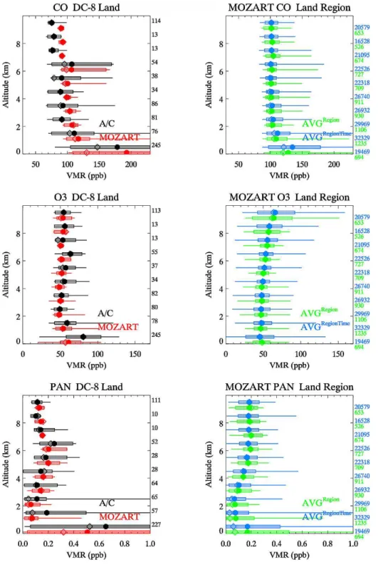
A comparison of observed and modeled vertical profiles for CO, O3and PAN is shown in Fig. 5. The model captures vertical gradients and overall concentrations well. Contrary to ocean data we see that concentrations generally increase in magnitude and variability towards the surface due to the influence of local sources. Elevated CO, O3and PAN con-centrations observed at around 6 km are fairly well reflected in the model results. As for the ocean data, the model in the FT has a high bias in CO and a low bias in O3. The mean difference in FT concentrations between modeled and observed flight track data is 8±16 ppbV (12±17%) for CO and –5±11 ppbV (–6±18%) for O3.
Fig. 5.As Fig. 2 but for DC-8 Land data sets and the data have been filtered for fire influence.
4 km. As seen from Table 5, where we list mean FT tracer contributions for selections with and without fire filtering, it can be noted that filtering for fire influence also reduces the FF US contributions in the FT from 3.7±4.7 ppbV to 2.3±1.8 ppbV. This filtering has little effect on contributions from other tracers.
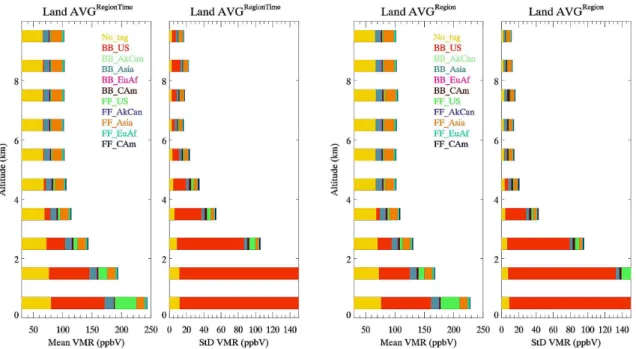
Fig. 6.As Fig. 4 but for AVGRegionTime and AVGRegion Land Data Sets.
indicates that the ocean flight was conducted on a day with above average pollution transport. Average FT CO concen-trations over land are 95±21 ppbV and 104±12 ppbV for observed and modeled flight track data, 103±9 ppbV for AVGRegionand 102±9 ppbV for AVGRegionTime. Average O3 concentrations are 57±12 ppbV, 51±6 ppbV, 50±9 ppbV, and 51±10 ppbV, respectively. The flight track model re-sults are underestimating the observed variability by a fac-tor of 2. The increased variability in O3for AVGRegionand AVGRegionTimesuggests that, at least for O3, the flight sam-pling was less representative for the large-scale variability.
3.3 Chemical boundary conditions from other data sets
As we have shown in the previous analysis, the chemical in-flow into the US West Coast is highly variable on spatial and temporal scales. Here we extend our analysis to three other observational data sets in order (1) to increase the sample size of observed chemical inflow conditions and gain a more complete picture of the existing variability, (2) to evaluate the boundary conditions flight for its representativeness in the context of other observations, and (3) to provide further evaluation of the modeled magnitude and variability. Addi-tional data sets include CO and O3retrievals from the Tro-pospheric Emissions Spectrometer (TES) onboard the NASA EOS Aura satellite, CO and O3aircraft measurements from the MOZAIC program on flights into Los Angeles, Califor-nia and Portland, Oregon, and O3sonde launches at Trinidad Head.
Table 5. Average CO Source Contributions for AVGRegionTime
Land and the 2–8 km altitude range. Units are ppbV CO.
Land ALL Land noFire
NoTag 68.4±6.3 66.9±3.9 BB US 11.4±45.1 0.5±0.8 BB AKCan 0.0±0.0 0.0±0.0 BB Asia 9.9±3.0 9.6±3.0 BB EuAf 0.8±0.1 0.9±0.1 BB Cam 2.1±2.2 2.2±2.3 FF US 3.7±4.7 2.3±1.8 FF AKCan 0.1±0.1 0.1±0.1 FF Asia 15.8±4.4 15.9±4.6 FF EuAf 2.7±0.8 2.7±0.8 FF Cam 1.3±1.3 1.4±1.4
3.3.1 TES satellite retrievals
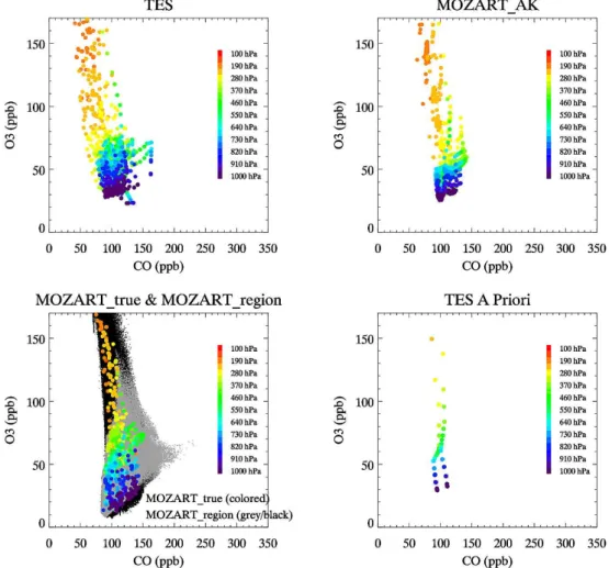
Fig. 7.As Fig. 3, but for TES CO and O3retrievals. Retrievals over Ocean (130–150 W, 30–45 N) for 15–30 June 2008. MOZART has been interpolated to the time, location and pressure grid (MOZART true) and convolved with the TES Averaging Kernels (MOZART AK). The bottom left panel further includes MOZART data for the entire region and time period with data within the 850–350 mbar range colored in gray (MOZART region). The bottom right panel shows scatter plots for the TES a priori CO and O3profiles.
For the following analysis only daytime TES retrievals with a degree of freedom of signal (DFS) larger than 1 and an average cloud optical depth<0.1 are included. Further selection criteria include a retrieval quality flag of 1 and a check of the O3C-Curve quality flag to eliminate unphysical O3retrievals (Osterman et al., 2009). In total this gives 61 coincident CO and O3profiles. Interpretation of satellite re-trievals is not as straightforward as for in-situ measurements. The retrieved profiles, while reported at specific vertical lev-els, represent averages over a broad range of the atmosphere with the vertical sensitivity expressed by the averaging ker-nels. To present the results in a manner comparable to the DC-8 data, we include in the following analysis the reported 11 retrieval levels between 850–350 hPa. However, it must be kept in mind that the retrievals have about 1–2 DFS and therefore the vertical levels are not independent of each other. Results for CO to O3relationships, similar to those shown for the DC-8 aircraft data in Fig. 3, are shown in Fig. 7. In comparing the two figures it must be kept in mind that
Fig. 8.As Fig. 3 but for MOZAIC CO and O3data. The location of the MOZAIC profile measurements for June and July of 2004–2008 is shown in the map.
Following the analysis of the ARCTAS-CARB aircraft data, we also list percentiles for TES and correspond-ing model results in Table 2. Lacking observational ev-idence, we do not list fifiltered statistics for TES re-trievals and corresponding MOZART AK results, but do so for MOZART true and MOZART region following the same filtering of model results as before. Fires have a small influ-ence on the model statistics for TES sampling. The TES– MOZART comparison leads to conclusions similar to those from the analysis of the aircraft data, even though the TES sensitivity has a smoothing effect on the measured and mod-eled values.
The model represents the main correlations seen in the TES data, but shows a smaller range, less variability and misses some of the retrievals with increased CO and O3. Overall the model, in agreement with the previous evalua-tion results, shows a mean positive bias compared to the TES CO retrievals of 2±15 ppbV (3±14%) and a mean nega-tive bias compared to the TES O3retrievals of –8±10 ppbV (–11±21 %). The smoothing effect of the TES operator re-duces the variability from 17 ppbV to 13 ppbV for CO and from 14 ppbV to 7 ppbV for O3. Comparing MOZART true to the sampling for the entire region (MOZART region) we see in the latter more elevated CO/O3plumes (Fig. 7). In a statistical sense (Table 2), however, these points have small weight and the statistics for the TES sampling gives an over-all good representation of the temporal and spatial average with comparable means and medians for CO, but somewhat enhanced O3mean and medians.
nia as an additional diagnostic for the representativeness of the ARCTAS/CARB boundary conditions flight. MOZAIC profiles over California are rare and to increase the sample size we look at all MOZAIC profiles collected in June or July during 2004–2008. In total we have 100 profiles, split about evenly between Portland and Los Angeles. For the Trinidad Head ozonesonde data we include all launches during June and July over the 10-year period 2000–2009. In total this gives 123 profiles. A time and space interpolated compari-son of MOZAIC and ozonecompari-sonde data with model results is not included, because the simulations do not cover the mea-surement time period.
A scatter plot for the CO-O3relationships from MOZAIC data for 2–8 km is shown in Fig. 8 and the locations of the available profiles over Los Angeles and Portland are also il-lustrated. The related percentiles are listed in Table 2. The MOZAIC data show a larger number of data points with a strong increase in CO and moderate increase in O3 represen-tative of fresh plumes. This is expected as the low altitude MOZAIC data are sampled over land on approach to airports in populated areas. Most of the fresh plumes were encoun-tered at low altitudes, but there are a few points above 2 km reflecting fresh pollution characteristics (light blue points in Fig. 8). Overall, fresh continental pollution should have lit-tle impact on free tropospheric statistics. Some data points replicate the correlations of moderate CO and strong O3 in-creases as were seen in the DC-8 sampling, but at even higher altitudes.
Fig. 9. Mean and standard deviation of vertical profiles for CO, O3and PAN from the different data sets DC8-Ocean (blue), DC-8 Land (red), MOZAIC (green) and ozonesondes (orange). Observations are shown in thick solid lines, and MOZART regional averages (AVGRe-gionTime) in dotted lines. The ensemble mean observed profile is denoted by symbols. For altitudes<2 km the ensemble mean is derived from DC-8 Ocean and ozonesonde data only. Except for MOZAIC and sonde data, the data have been filtered for fire influence.
The 10–90% range for O3 is 47 ppbV for MOZAIC and 49 ppbV for the sonde data, which is similar to the DC-8 sampling (54 ppbV). Median and mean concentrations are slightly lower compared to DC-8 Ocean data, and closer to DC-8 Land sampling. Mean FT concentrations for MOZAIC O3are 62±19 ppbV and 61±20 ppbV for the ozonesonde. Due to the pristine location of Trinidad Head, we also assess the sonde profiles at low altitudes for their representative-ness of background concentrations and marine air. As shown in Table 3, the ozonesonde statistics over the 0–1 km altitude range are similar to the mean and median statistics calculated for the DC-8 Ocean data set. This confirms that Trinidad Head is a well-suited location for detecting background con-ditions and the value of using sonde measurements in exam-ining inflow.
3.4 Average Chemical BC from in-situ measurements and MOZART
Fig. 10. Daily average difference in surface O3(ppbV) between the WRF-Chem simulations with temporally varying and with temporally averaged chemical boundary conditions (variable BC minus mean BC).
clearly higher for observations compared to the model. The high concentrations at high altitudes for the DC-8 ocean flight are exceptional, and this supports our previous con-clusion that the DC-8 boundary conditions flight captured a more pronounced episode of long-range pollution transport than is usual. Aside from the lowermost altitudes, the aircraft measurements over land show no significant bias compared to the ocean data, again confirming that free tropospheric ob-servations over land may be considered as representative of pollution inflow as long as caution is taken not to interpret lofted local pollution as pollution inflow.
We include in the graphs also the ensemble mean of all observational data sets. For the lowest 2 km we consider the DC-8 ocean data set and MOZAIC data only to avoid the influence of local pollution sources. For regional mod-els, which are not designed to incorporate time and space varying boundary conditions or if boundary conditions from global models are not available with sufficient confidence, we suggest this ensemble mean might be used for a proper approximation of average inflow conditions. The ensemble mean does replicate vertical profiles typical for air masses over ocean, i.e. little vertical variability in CO and
decreas-ing concentrations towards the surface for O3and PAN. The average “background” conditions for CO are on the order of 100 ppbV, for O3 on the order of 25 ppbV near the surface increasing to 55 ppbV in the mid-troposphere, and for PAN about 0.02 ppbV at the surface approaching 0.2 ppbV at alti-tudes of 6 km and higher.
4 Influence of the variability in chemical BC in a regional model
Fig. 11.Left hand side: RMS difference in surface O3between the WRF-Chem simulations with temporally varying and with temporally averaged chemical boundary conditions. Right hand side: Elevation (m) over the regional domain.
the WRF-Chem simulation (14–30 June 2008). Both simula-tions start from the same initial condisimula-tions and model fields are output every two hours. The mean and standard deviation of the CO and O3chemical inflow for “Variable BC” (this is represented by AVGRegionTime for Ocean without fire filter-ing) is 104±14 ppbV and 50±12 ppbV, respectively. The 10–90th range spanned by the model results is 27 ppbV for CO and 28 ppbV for O3. In comparison, for the “Mean BC” scenario CO and O3mean concentrations (applying the same averaging as for AVGRegionTime to the mean modeled fields) are 104±4 ppbV and 50±4 ppbV with 10–90% ranges of 11 ppbV and 11 ppbV, respectively (Table 2). In other words, the variability and range in the inflow is reduced by a factor of nearly 3 for the mean BC simulation compared to the vari-able BC simulation. While beyond the scope of this study, we present in the Supplement, analogous to Figs. 2, 3 and 5, a comparison of MOZART and WRF-Chem results to the aircraft data.
In Fig. 10 we present maps of daily average difference in surface O3 between the “Variable BC” and the “Mean BC” simulation. During the first days of the simulations differ-ences are mostly seen around the outer edges of the do-main, but after three days we see clear changes in the sur-face concentrations throughout the domain aproaching about ±15 ppbV over California with a large spatial and temporal variability. Figure 11 shows the root mean square (RMS) dif-ference for the entire simulation period together with a map of the domain topography. High altitude locations commonly are expected to show the largest sensitivity to pollution in-flow and are considered as most representative for pollution inflow. However, our results show the largest RMS differ-ences (up to 5 ppbV) not necessarily at the high altitudes, but in the Central Valley region, which is a lower altitude area. A similar pattern is also seen for the RMS differences in sur-face CO (not shown here). Varying concentrations of O3in
onshore flow have recently been shown to have a strong in-fluence on measured surface O3concentrations in the Central Valley. Parrish et al. (2010) found that measured surface O3 concentrations correlate with the O3measured in the lower free troposphere by the Trinidad Head sondes after allow-ing for a time delay of approximately 20 h. On days that surface O3exceeded the air quality standard of 75 ppbv, the transported O3as measured by the sondes averaged 11 ppbv higher compared to days with lower O3observed at the sur-face.
Histograms of the percentage differences between “Vari-able BC” and “Mean BC” simulations for surface concentra-tions for O3, CO, NOxand PAN over California are shown in Fig. 12. CO and NOx, which are strongly source driven and as such highest near local emission sources, show smaller rel-ative changes compared to the more photochemically driven species O3and PAN, which are formed photochemically dur-ing transport. The frequency of cases where changes amount to ±10% or more are 9% for O3, 11.5% for PAN, and∼1% for CO and NOx.
Fig. 12. Histograms in the percentage difference between surface concentrations of O3, CO, NOxand PAN over California between the WRF-Chem simulations with temporally varying and with tem-porally averaged chemical boundary conditions.
only California surface data where the BC have a distinct influence (absolute difference in surface O3between “Vari-able BC” and “Mean BC” >3 ppbV, which includes 12% of all surface data over California), the daily 8-h maximum O3concentrations exceeded 75 ppbV (65 ppbV) in the “Vari-able BC” simulation on 10% (25%) of the days modeled. In the “Mean BC” simulation, these frequencies were reduced to 8% (18%). It must be considered that these statistics may not quite represent a typical influence of pollution inflow. The considered time period was significantly impacted by the intense wildfires, which may have in parts mitigated the in-fluence of pollution inflow. However, the estimated sensitivi-ties might even be on the lower end during strong long-range pollution events, which, as was discussed in Sect. 3.1, are strongly underestimated in a global model.
5 Conclusions
We have presented an analysis of measurements of the long-lived tracers CO, O3and PAN combined with global model simulations to examine the characteristics of airmasses enter-ing the US West Coast. The data sets were collected on four platforms: the NASA-DC8 aircraft during ARCTAS-CARB in June 2008 (with all three species measured), the TES satel-lite (CO and O3), MOZAIC aircraft (CO and O3)and O3 son-des launched from Trinidad Head, California. Both observa-tions and models reflect a large variability in pollution in-flow on temporal and spatial scales, but the MOZART global model captured only about half of the observed free tropo-spheric variability. Sensitivity studies with a regional model demonstrate that the representation of the variability in
pol-from global models provide useful input to regional models, but likely still lead to an underestimate of peak surface con-centrations associated with long-range pollution transport. It therefore is important to carefully evaluate the chemical boundary conditions implemented in regional air quality sim-ulations not only for their representation of the overall back-ground, but also for their representativeness of spatial and temporal variability and frequency distributions.
Model tracer contributions show a large contribution from Asian emissions on FT air masses. Local US pollution can impact chemical boundary conditions both by recirculation within the eastern Pacific region, and by around-the-world transport in the case of long-lived tracers. This emphasizes the importance of consistency between the global model sim-ulations used for boundary conditions and the regional model in terms of emissions, chemistry and transport. To mitigate the influence of the boundary conditions, nested regional do-mains with a sufficiently large outer domain are an option but not always possible as they involve a large computational demand.
Aircraft measurements in the free troposphere over Cal-ifornia show similar concentration range, variability and source contributions as free tropospheric air masses over ocean, but caution has to be taken that lofted local pollu-tion is not misinterpreted as inflow. In the case of the June 2008 period the intense wildfire pollution was seen to have a significant impact on the free troposphere over land. The es-pecially designed boundary conditions flight conducted dur-ing ARCTAS-CARB showed an above average prevalence of plumes transported from Asia and thus may not be fully representative for average inflow conditions.
Owing to the large variability in atmospheric transport, more frequent free tropospheric measurements are needed to better characterize pollution inflow and to evaluate and im-prove (e.g. through model imim-provements and/or data assimi-lation) chemical boundary conditions used in regional model simulations. The evaluation of boundary conditions must be a crucial part of regional model evaluation, especially for re-gions like California where pollution inflow embodies a sig-nificant contribution to air quality.
Supplementary material related to this article is available online at:
http://www.atmos-chem-phys.net/11/1769/2011/ acp-11-1769-2011-supplement.pdf.
Acknowledgements. The authors like to acknowledge Ajith
to thank the reviewers for their constructive comments and sugges-tions. Acetonitrile measurements were supported by the Austrian Research Promotion Agency (FFG-ALR) and the Tiroler Zukun-ftstiftung and carried out with the help/support of T. Mikoviny, M. Graus, A. Hansel and T. D. Maerk. The authors acknowledge the strong support of the European Commission, Airbus, and the Airlines (Lufthansa, Austrian, Air France) who carry free of charge the MOZAIC equipment and perform the maintenance since 1994. MOZAIC is presently funded by INSU-CNRS (France), Meteo-France, and Forschungszentrum (FZJ, Julich, Germany). The MOZAIC data based is supported by ETHER (CNES and INSU-CNRS). The research was supported by NASA grants NNX10AH45G, NNX08AD22G and NNX07AL57G. NCAR is operated by the University Corporation of Atmospheric Research under sponsorship of the National Science Foundation.
Edited by: A. Stohl
References
Beer, R.: TES on the Aura mission: Scientific objectives, mea-surements, and analysis overview, IEEE Trans. Geosci. Remote Sens., 44 (5), 1102–1105, 2006.
Bertschi, I. T., Jaffe, D. A., Jaegl´e, L., Price, H. U., and Denni-son, J. B.: PHOBEA/ITCT 2002 25 airborne observations of transpacific transport of ozone, CO, volatile organic compounds, and aerosols to the northeast Pacific: Impacts of Asian anthro-pogenic and Siberian boreal fire emissions, J. Geophys. Res., 109, D23S12, doi:10.1029/2003JD004328, 2004.
Brown, J. A., Jr.: Operational numerical weather prediction, Rev. Geophys., 25(3), 312–322, doi:10.1029/RG025i003p00312, 1987.
Chin, M., Ginoux, P., Kinne, S. Holben, B. N., Duncan, B. N, Mar-tin, R. V., Logan, J. A, Higurashi, J., and Nakajima, T.: Tropo-spheric aerosol optical thickness from the GOCART model and comparisons with satellite and sunphotometer measurements, J. Atmos. Sci. 59, 461–483, 2002.
Diskin, G. S., Podolske, J. R., Sachse, G. W., and Slate, T. A.: Open-Path Airborne Tunable 15 Diode Laser Hygrometer, in Diode Lasers and Applications in Atmospheric Sensing, SPIE Proceedings 4817, A. Fried, ed., 196–204, 2002.
Ek, M. B., Mitchell, K. E. Lin, Y., Rogers, E., Grunmann, P., Ko-ren, V., Gayno, G., and Tarpley, J. D.: Implementation of Noah land surface model advances in the National Centers for Environ-mental Prediction operational mesoscale Eta model, J. Geophys. Res., 108(D22), 8851, doi:10.1029/2002JD003296, 2003. Emmons, L. K., Walters, S., Hess, P. G., Lamarque, J.-F., Pfister,
G. G., Fillmore, D., Granier, C., Guenther, A., Kinnison, D., Laepple, T., Orlando, J., Tie, X., Tyndall, G., Wiedinmyer, C., Baughcum, S. L., and Kloster, S.: Description and evaluation of the Model for Ozone and Related chemical Tracers, version 4 (MOZART-4), Geosci. Model Dev., 3, 43–67, doi:10.5194/gmd-3-43-2010, 2010a.
Emmons, L. K., Apel, E. C., Lamarque, J.-F., Hess, P. G., Avery, M., Blake, D., Brune, W., Campos, T., Crawford, J., DeCarlo, P. F., Hall, S., Heikes, B., Holloway, J., Jimenez, J. L., Knapp, D. J., Kok, G., Mena-Carrasco, M., Olson, J., O’Sullivan, D., Sachse, G., Walega, J., Weibring, P., Weinheimer, A., and Wiedinmyer, C.: Impact of Mexico City emissions on regional air quality from
MOZART-4 simulations, Atmos. Chem. Phys., 10, 6195–6212, doi:10.5194/acp-10-6195-2010, 2010b.
Fast, J., Aiken, A. C., Allan, J., Alexander, L., Campos, T., Cana-garatna, M. R., Chapman, E., DeCarlo, P. F., de Foy, B., Gaffney, J., de Gouw, J., Doran, J. C., Emmons, L., Hodzic, A., Hern-don, S. C., Huey, G., Jayne, J. T., Jimenez, J. L., Kleinman, L., Kuster, W., Marley, N., Russell, L., Ochoa, C., Onasch, T. B., Pekour, M., Song, C., Ulbrich, I. M., Warneke, C., Welsh-Bon, D., Wiedinmyer, C., Worsnop, D. R., Yu, X.-Y., and Zaveri, R.: Evaluating simulated primary anthropogenic and biomass burning organic aerosols during MILAGRO: implications for as-sessing treatments of secondary organic aerosols, Atmos. Chem. Phys., 9, 6191–6215, doi:10.5194/acp-9-6191-2009, 2009. Fiore, A. M., Dentener, F. J., Wild, O., Cuvelier, C., Schultz, M. G.,
Hess, P., Textor, C., Schulz, M., Doherty, R. M., Horowitz, L. W., MacKenzie, I. A., Sanderson, M. G., Shindell, D. T., Steven-son, D. S., Szopa, S., Van Dingenen, R., Zeng, G., Atherton, C., Bergmann, D., Bey, I., Carmichael, G., Collins, W. J., Duncan, B. N., Faluvegi, G., Folberth, G., Gauss, M., Gong, S., Hauglus-taine, D., Holloway, T., Isaksen, I. S. A., Jacob, D. J., Jonson, J. E., Kaminski, J. W., Keating, T. J., Lupu, A., Marmer, E., Montanaro, V., Park, R. J., Pitari, G., Pringle, K. J., Pyle, J. A., Schroeder, S., Vivanco, M. G., Wind, P., Wojcik, G., Wu, S., and Zuber, A.: Multimodel estimates of intercontinental source-receptor relationships for ozone pollution, J. Geophys. Res., 114, D04301, doi:10.1029/2008JD010816, 2009.
Freitas, S. R., Longo, K. M., Chatfield, R., Latham, D., Silva Dias, M. A. F., Andreae, M. O., Prins, E., Santos, J. C., Gielow, R., and Carvalho Jr., J. A.: Including the sub-grid scale plume rise of vegetation fires in low resolution atmospheric transport models, Atmos. Chem. Phys., 7, 3385–3398, doi:10.5194/acp-7-3385-2007, 2007.
Granier, C., Mueller, J. F., Petron, G. and Brasseur, G.: A three-dimensional study of the CO budget, Glob. Change Science, 1, 255–261, 1999.
Grell, G. A., Peckham, S. E., Schmitz, R., McKeen, S. A., Frost, G., Skamarock, W. C., and Eder, B.: Fully coupled online chemistry within the WRF model, Atmos. Environ., 39, 6957–6975, 2005. Guenther, A., Karl, T., Harley, P., Wiedinmyer, C., Palmer, P. I., and Geron, C.: Estimates of global terrestrial isoprene emissions using MEGAN (Model of Emissions of Gases and Aerosols from Nature), Atmos. Chem. Phys., 6, 3181–3210, doi:10.5194/acp-6-3181-2006, 2006.
Heald, C. L., Jacob, J., Fiore, A. M., Emmons, L. K., Gille, J. C., Deeter, M. N., Warner, J., Edwards, D. P., Crawford, J. H., Ham-lin, A. J., Sachse, G. W., Browell, E. V., Avery, M. A., Vay, S. A., Westberg, D. J., Blake, D. R., Singh, H. B., Sandholm, S. T., Talbot, R. W., and Fuelberg, H. E.: Asian outflow and trans-Pacific transport of carbon monoxide and ozone pollution: An integrated satellite, aircraft, and model perspective, J. Geophys. Res., 108(D24), 17, 4804, doi:10.1029/2003JD003507, 2003. Hess, P. G. and Lamarque, J. F.: Ozone source attribution and its
modulation by the Arctic oscillation during the spring months, J. Geophys. Res., 112, D11303, doi:10.1029/2006JD007557, 2007. Horowitz, L., Walters, S., and Mauzerall, D.S.: A global simula-tion of tropospheric ozone and related tracers: Descripsimula-tion and evaluation of MOZART, version 2, J. Geophys. Res., 108, 4784, 25 pp., doi:10.1029/2002JD002853, 2003.
Impacts of transported background ozone on California air qual-ity during the ARCTAS-CARB period – a multi-scale modeling study, Atmos. Chem. Phys., 10, 6947–6968, doi:10.5194/acp-10-6947-2010, 2010.
Jacob, D. J., Crawford, J. H., Maring, H., Clarke, A. D., Dibb, J. E., Emmons, L. K., Ferrare, R. A., Hostetler, C. A., Russell, P. B., Singh, H. B., Thompson, A. M., Shaw, G. E., McCauley, E., Ped-erson, J. R., and Fisher, J. A.: The Arctic Research of the Com-position of the Troposphere from Aircraft and Satellites (ARC-TAS) mission: design, execution, and first results, Atmos. Chem. Phys., 10, 5191–5212, doi:10.5194/acp-10-5191-2010, 2010. Jacob, D. J., Logan, J. A., and Murti, P. P.: Effect of rising Asian
emissions on surface ozone in the United States, Geophys. Res. Lett., 26(14), 2175–2178, 1999.
Janjic, Z. I.: Nonsingular Implementation of the Mellor-Yamada Level 2.5 Scheme in the NCEP Meso model. NCEP Office Note No. 437, 61 pp., 2002.
Johnson, B. J., Oltmans, S. J., Voemel, H., Smit, H. G. J., Desh-ler, T., and Kr¨oger, C.: Electrochemical concentration cell (ECC) ozonesonde pump efficiency measurements and tests on the sensitivity to ozone of buffered and unbuffered ECC sensor cathode solutions, J. Geophys. Res., 107(D19), 4393, doi:10.1029/2001JD000557, 2002.
Jourdain, L., Worden, H. M., Worden, J. R., Bowman, K., Li, Q., El-dering, A., Kulawik, S. S., Osterman, G., Boersma, K. F., Fisher, B., Rinsland, C. P., Beer, R., and Gunson, M.: Tropospheric ver-tical distribution of tropical Atlantic ozone observed by TES dur-ing the Northern African biomass burndur-ing season, Geophys. Res. Lett., 34, L04810, doi:10.1029/2006GL028284, 2007.
Lamarque, J.-F., Hess, P., Emmons, L., Buja, L., Washing-ton, W., and Granier, C.: Tropospheric ozone evolution between 1890 and 1990, J. Geophys. Res., 110, D08304, doi:10.1029/2004JD005537, 2005.
Li, Q., Jacob, D. J., Palmer, P. I, Duncan, B. N., Field, B. D., Fiore, A. M., Yantosca, R. M., Parrish, D. D., Simmonds, P. G., and Oltsman S.: Transatlantic transport of pollution and its effects on surface ozone in Europe and North America, J. Geophys. Res., 107, doi:10.1029/2001JD001422, 2002.
Li, Q., Jacob, D. J. Munger, J. W., Yantosca, R. M, and Parrish, D. D.: Export of NOy from the North American boundary layer: Reconciling aircraft observations and global model budgets, J. Geophys. Res., 109, D02313, doi:10.1029/2003JD004086, 2004. Lin, M., Holloway, T., Carmichael, G. R., and Fiore, A. M.: Quan-tifying pollution inflow and outflow over East Asia in spring with regional and global models, Atmos. Chem. Phys., 10, 4221– 4239, doi:10.5194/acp-10-4221-2010, 2010.
Lopez, J. P., Luo, M., Christensen, L. E., Loewenstein, M., Jost, H., Webster, C. R., and Osterman, G.: TES carbon monoxide valida-tion during two AVE campaigns using the Argus and ALIAS in-struments on NASA’s WB-57F, J. Geophys. Res., 113, D16S47, doi:10.1029/2007JD008811, 2008.
Luo, M., Rinsland, C., Fisher, B., Sachse, G., Diskin, G., Logan, J., Worden, H., Kulawik, S., Osterman, G., Eldering, A., Herman, R., and Shephard, M.: TES carbon monoxide validation with DACOM aircraft measurements during INTEX-B 2006, J. Geo-phys. Res., 112, D24S48, doi:10.1029/2007JD008803, 2007.
and water vapour by Airbus in-service aircraft: The MOZAIC airborne program, an overview, J. Geophys. Res., 103, 25631– 25642, 1998.
Mena-Carrasco, M., Carmichael, G. R., Campbell, J. E., Zimmer-man, D., Tang, Y., Adhikary, B., Dallura, A., Molina, L. T., Zavala, M., Garca, A., Flocke, F., Campos, T., Weinheimer, A. J., Shetter, R., Apel, E., Montzka, D. D., Knapp, D. J., and Zheng, W.: Assessing the regional impacts of Mexico City emissions on air quality and chemistry, Atmos. Chem. Phys., 9, 3731–3743, doi:10.5194/acp-9-3731-2009, 2009.
Nassar, R., Logan, J. A., Worden, H., Megretskaia, I. A., Bow-man, K. W., OsterBow-man, G. B., Thompson, A. M., Tarasik, D. W., Austin, S., Claude, H.,Dubey, M. K.,Hocking, W. K., John-son, B. J., Joseph, E., Merrill, J., Morris, G. A., Newchurch, M., Oltmans, S. J., Posny, F., Schmidlin, F. J., Voemel, H., Whiteman, D. N., and Witte, J. C.: Validation of Tropo-spheric Emission Spectrometer (TES) nadir ozone profiles us-ing ozonesonde measurements, J. Geophys. Res., 113, D15S17, doi:10.1029/2007JD008819, 2008.
Nedelec, P., Cammas, J.-P., Thouret, V., Athier, G., Cousin, J.-M., Legrand, C., Abonnel, C., Lecoeur, F., Cayez, G., and Marizy, C.: An improved infrared carbon monoxide analyser for routine measurements aboard commercial Airbus aircraft: technical val-idation and first scientific results of the MOZAIC III programme, Atmos. Chem. Phys., 3, 1551–1564, doi:10.5194/acp-3-1551-2003, 2003.
Oltmans, S. J., Lefohn, A. S., Harris, J. M., and Shadwick, D. S.: Background ozone levels of air entering the west coast of the US and assessment of longer-term changes, Atmos. Environ., 42, 6020–6038, 2008.
Osterman, G., Kulawik, S., Worden, H., Richards, N., Fisher, B., Eldering, A., Shephard, M., Froidevaux, L., Labow, G., Luo, M., Herman, R., and Bowman, K.: Validation of Tropospheric Emission Spectrometer (TES) Measurements of the Total, Strato-spheric and TropoStrato-spheric Column Abundance of Ozone, J. Geo-phys. Res., 113, D15S16, doi:10.1029/2007JD008801, 2008. Osterman, G. (Ed.), Bowman, K., Eldering, A., Fisher, B., Herman,
R., Jacob, D., Jourdain, L., Kuawik, S., Luo, M., Monarrez, R., Paradise, S., Payne, V., Poosti, S., Richards, N., Rider, D., 5 Shephard, D., Shephard, M., Vilntotter, F., Worden, H., Worden, J., Yun, H., and Zhang, L.: TES Level 2 Data Users Guide, v4.0, JPL D-38042, 20 May 2009, available at: http://tes.jpl.nasa.gov/ documents/, 2009.
Parrish, D. D., Holloway, J. S., Trainer, M., Murphy, P. C., Fehsen-feld, F. C., and Forbes, G. L.: Export of North America ozone pollution to the North Atlantic Ocean, Science, 259(5100), 1436–1439, 1993.
Parrish, D. D., Aikin, K. C., Oltmans, S. J., Johnson, B. J., Ives, M., and Sweeny, C.: Impact of transported background ozone in-flow on summertime air quality in a California ozone exceedance area, Atmos. Chem. Phys., 10, 10093–10109, doi:10.5194/acp-10-10093-2010, 2010.