Sources, seasonality, and trends of Southeast US aerosol: an integrated analysis of surface, aircraft, and satellite observations with the GEOS-Chem chemical transport model

ACPD

Sources, seasonality,

and trends of

Southeast US aerosol

P. S. Kim et al.

Title Page

Abstract Introduction

Conclusions References

Tables Figures

◭ ◮

◭ ◮

Back Close

Full Screen / Esc

Printer-friendly Version Interactive Discussion

Discussion

P

a

per

|

Discussion

P

a

per

|

Discussion

P

a

per

|

Discussion

P

a

per

|

Atmos. Chem. Phys. Discuss., 15, 17651–17709, 2015 www.atmos-chem-phys-discuss.net/15/17651/2015/ doi:10.5194/acpd-15-17651-2015

© Author(s) 2015. CC Attribution 3.0 License.

This discussion paper is/has been under review for the journal Atmospheric Chemistry and Physics (ACP). Please refer to the corresponding final paper in ACP if available.

Sources, seasonality, and trends of

Southeast US aerosol: an integrated

analysis of surface, aircraft, and satellite

observations with the GEOS-Chem

chemical transport model

P. S. Kim

, D. J. Jacob

, J. A. Fisher

, K. Travis

, K. Yu

, L. Zhu

,

R. M. Yantosca

, M. P. Sulprizio

, J. L. Jimenez

, P. Campuzano-Jost

,

K. D. Froyd

, J. Liao

, J. W. Hair

, M. A. Fenn

, C. F. Butler

, N. L. Wagner

,

T. D. Gordon

, A. Welti

, P. O. Wennberg

, J. D. Crounse

,

J. M. St. Clair

, A. P. Teng

, D. B. Millet

, J. P. Schwarz

, M. Z. Markovic

,

and A. E. Perring

1

Department of Earth and Planetary Sciences, Harvard University, Cambridge, MA, USA

2

School of Engineering and Applied Sciences, Harvard University, Cambridge, MA, USA

3

School of Chemistry, University of Wollongong, Wollongong, New South Wales, Australia

4

ACPD

Sources, seasonality,

and trends of

Southeast US aerosol

P. S. Kim et al.

Title Page

Abstract Introduction

Conclusions References

Tables Figures

◭ ◮

◭ ◮

Back Close

Full Screen / Esc

Printer-friendly Version Interactive Discussion

Discussion

P

a

per

|

Discussion

P

a

per

|

Discussion

P

a

per

|

Discussion

P

a

per

|

5

Department of Chemistry and Biochemistry, University of Colorado Boulder, Boulder, CO, USA

6

Chemical Sciences Division, National Oceanic and Atmospheric Administration Earth System Research Laboratory, Boulder, CO, USA

7

NASA Langley Research Center, Hampton, VA, USA

8

Science Systems and Applications, Inc., Hampton, VA, USA

9

Institute for Atmospheric and Climate Science, Swiss Federal Institute of Technology, Zurich, Switzerland

10

Division of Geological and Planetary Sciences, California Institute of Technology, Pasadena, CA, USA

11

Division of Engineering and Applied Science, California Institute of Technology, Pasadena, CA, USA

12

Deparment of Soil, Water, and Climate, University of Minnesota, Minneapolis-Saint Paul, MN, USA

a

now at: Atmospheric Chemistry and Dynamics Laboratory, NASA Goddard Space Flight Center, Greenbelt, MD, USA

b

now at: Joint Center for Earth Systems Technology, University of Maryland Baltimore County, Baltimore, MD, USA

c

now at: Air Quality Research Division, Environment Canada, Toronto, Ontario, Canada Received: 05 May 2015 – Accepted: 10 June 2015 – Published: 01 July 2015

Correspondence to: P. S. Kim (kim68@fas.harvard.edu)

ACPD

Sources, seasonality,

and trends of

Southeast US aerosol

P. S. Kim et al.

Title Page

Abstract Introduction

Conclusions References

Tables Figures

◭ ◮

◭ ◮

Back Close

Full Screen / Esc

Printer-friendly Version Interactive Discussion

Discussion

P

a

per

|

Discussion

P

a

per

|

Discussion

P

a

per

|

Discussion

P

a

per

|

Abstract

We use an ensemble of surface (EPA CSN, IMPROVE, SEARCH, AERONET), aircraft

(SEAC

RS), and satellite (MODIS, MISR) observations over the Southeast US during

the summer-fall of 2013 to better understand aerosol sources in the region and the

relationship between surface particulate matter (PM) and aerosol optical depth (AOD).

5

The GEOS-Chem global chemical transport model (CTM) with 25 km

×

25 km

resolu-tion over North America is used as a common platform to interpret measurements of

di

_ff

erent aerosol variables made at di

_ff

erent times and locations. Sulfate and organic

aerosol (OA) are the main contributors to surface PM

(mass concentration of PM

finer than 2.5 µm aerodynamic diameter) and AOD over the Southeast US.

GEOS-10

Chem simulation of sulfate requires a missing oxidant, taken here to be stabilized

Criegee intermediates, but which could alternatively reflect an unaccounted for

het-erogeneous process. Biogenic isoprene and monoterpenes account for 60 % of OA,

anthropogenic sources for 30 %, and open fires for 10 %. 60 % of total aerosol mass

is in the mixed layer below 1.5 km, 20 % in the cloud convective layer at 1.5–3 km, and

15

20 % in the free troposphere above 3 km. This vertical profile is well captured by

GEOS-Chem, arguing against a high-altitude source of OA. The extent of sulfate neutralization

(

f

=

[NH

]

/

(2[SO

]

+

[NO

])) is only 0.5–0.7 mol mol

in the observations, despite an

excess of ammonia present, which could reflect suppression of ammonia uptake by

organic aerosol. This would explain the long-term decline of ammonium aerosol in the

20

Southeast US, paralleling that of sulfate. The vertical profile of aerosol extinction over

the Southeast US follows closely that of aerosol mass. GEOS-Chem reproduces

ob-served total column aerosol mass over the Southeast US within 6 %, column aerosol

extinction within 16 %, and space-based AOD within 21 %. The large AOD decline

ob-served from summer to winter is driven by sharp declines in both sulfate and OA from

25

ACPD

Sources, seasonality,

and trends of

Southeast US aerosol

P. S. Kim et al.

Title Page

Abstract Introduction

Conclusions References

Tables Figures

◭ ◮

◭ ◮

Back Close

Full Screen / Esc

Printer-friendly Version Interactive Discussion

Discussion

P

a

per

|

Discussion

P

a

per

|

Discussion

P

a

per

|

Discussion

P

a

per

|

SEAC4RS aircraft data demonstrate that AODs measured from space are

fundamen-tally consistent with surface PM

. This implies that satellites can be used reliably

to infer surface PM

over monthly timescales if a good CTM representation of the

aerosol vertical profile is available.

1

Introduction

5

There is considerable interest in using satellite retrievals of aerosol optical depth (AOD)

to map particulate matter concentrations (PM) in surface air and their impact on public

health (Liu et al., 2004; Zhang et al., 2009; van Donkelaar et al., 2010, 2015; Hu et al.,

2014). The relationship between PM and AOD is a function of the vertical distribution

and optical properties of the aerosol. It is generally derived from a global chemical

10

transport model (CTM) simulating the di

_ff

erent aerosol components over the depth of

the atmospheric column (van Donkelaar et al., 2012, 2013; Boys et al., 2014).

Sul-fate and organic matter are the dominant submicron aerosol components worldwide

(Murphy et al., 2006; Zhang et al., 2007; Jimenez et al., 2009), thus it is important to

evaluate the ability of CTMs to simulate their concentrations and vertical distributions.

15

Here we use the GEOS-Chem CTM to interpret a large ensemble of aerosol chemical

and optical observations from surface, aircraft, and satellite platforms during the NASA

SEAC

RS campaign in the Southeast US in August–September 2013. Our objective is

to better understand the relationship between PM and AOD, and the ability of CTMs to

simulate it, with focus on the factors controlling sulfate and organic aerosol (OA).

20

The Southeast US is a region of particular interest for PM air quality and for aerosol

radiative forcing of climate (Goldstein et al., 2009). PM

(the mass concentration of

particulate matter finer than 2.5 µm aerodynamic diameter, of most concern for public

health) is in exceedance of the current US air quality standard, 12 µg m

_{on an annual}

mean basis, in several counties (http://www.epa.gov/airquality/particlepollution/actions.

25

ACPD

Sources, seasonality,

and trends of

Southeast US aerosol

P. S. Kim et al.

Title Page

Abstract Introduction

Conclusions References

Tables Figures

◭ ◮

◭ ◮

Back Close

Full Screen / Esc

Printer-friendly Version Interactive Discussion

Discussion

P

a

per

|

Discussion

P

a

per

|

Discussion

P

a

per

|

Discussion

P

a

per

|

summertime (JJA) mean concentrations of aerosol components for 2003–2013 from

surface monitoring stations in the Southeast US managed by the US Environmental

Protection Agency (US EPA, 1999). Sulfate concentrations decreased by 60 % over

the period while OA concentrations decreased by 40 % (Hand et al., 2012a; Blanchard

et al., 2013; Hidy et al., 2014). Decreasing aerosol has been linked to rapid warming in

5

the Southeast US over the past two decades (Leibensperger et al., 2012a, b).

The sulfate decrease is driven by the decline of sulfur dioxide (SO

) emissions from

coal combustion (Hand et al., 2012a), though the mechanisms responsible for oxidation

of SO

to sulfate are not well quantified. Better understanding of the mechanisms is

im-portant because dry deposition competes with oxidation as a sink of SO

, so that faster

10

oxidation produces more sulfate (Chin and Jacob, 1996). Standard model mechanisms

assume that SO

is oxidized to sulfate by the hydroxyl radical (OH) in the gas phase

and by hydrogen peroxide (H

O

) and ozone in clouds (aqueous phase). A model

in-tercomparison by McKeen et al. (2007) for the Northeast US revealed a general failure

of models to reproduce observed sulfate concentrations, sometimes by a factor of 2

15

or more. This could reflect errors in oxidation mechanisms, oxidant concentrations,

or frequency of cloud processing. Laboratory data suggest that stabilized Criegee

in-termediates (SCIs) formed from alkene ozonolysis could be important SO

oxidants

(Mauldin et al., 2012; Welz et al., 2012), though their ability to produce sulfate may be

limited by competing reactions with water vapor (Chao et al., 2015; Millet et al., 2015).

20

The factors controlling OA are highly uncertain. OA originates from anthropogenic,

biogenic, and open fire sources (de Gouw and Jimenez, 2009). It is directly emitted as

primary OA (POA) and also produced in the atmosphere as secondary OA (SOA) from

oxidation of volatile organic compounds (VOCs). Current models cannot reproduce

observed OA variability, implying fundamental deficiencies in the model mechanisms

25

ACPD

Sources, seasonality,

and trends of

Southeast US aerosol

P. S. Kim et al.

Title Page

Abstract Introduction

Conclusions References

Tables Figures

◭ ◮

◭ ◮

Back Close

Full Screen / Esc

Printer-friendly Version Interactive Discussion

Discussion

P

a

per

|

Discussion

P

a

per

|

Discussion

P

a

per

|

Discussion

P

a

per

|

1994; Donahue et al., 2006), so that “biogenic” SOA may be enhanced in the presence

of anthropogenic POA and SOA (Weber et al., 2007). The SOA yield from VOC

oxida-tion also depends on the concentraoxida-tion of nitrogen oxide radicals (NO

≡

NO

+

NO

)

(Kroll et al., 2005, 2006; Chan et al., 2010; Hoyle et al., 2011; Xu et al., 2014). NO

in

the Southeast US is mostly from fossil fuel combustion and is in decline due to emission

5

controls (Russell et al., 2012), adding another complication in the relationship between

OA concentrations and anthropogenic sources. Oxidation of biogenic VOC by the NO

radical formed from anthropogenic NO

is also thought to be an important SOA source

in the Southeast US (Pye et al., 2010). Reactions of organic molecules with sulfate to

form organosulfates may also play a small role (Surratt et al., 2007; Liao et al., 2015).

10

Long-term PM

records for the Southeast US are available from the EPA CSN,

IMPROVE, and SEARCH networks of surface sites (Malm et al., 1994; Edgerton et al.,

2005; Solomon et al., 2014). Satellite measurements of AOD from the MODIS and

MISR instruments have been operating continuously since 2000 (Diner et al., 2005;

Remer et al., 2005; Levy et al., 2013). Both surface and satellite observations show

15

a strong aerosol seasonal cycle in the Southeast US, with a maximum in summer and

minimum in winter (Alston et al., 2012; Hand et al., 2012b; Ford and Heald, 2013).

Goldstein et al. (2009) observed that the amplitude of the seasonal cycle of PM

measured at surface sites (maximum

/

minimum ratio of

∼

1.5; Hand et al., 2012b) is

much smaller than the seasonal cycle of AOD measured from space (ratio of

∼

3–4;

20

Alston et al., 2012). They hypothesized that this could be due to a summertime source

of biogenic SOA aloft. Subsequent work by Ford and Heald (2013) supported that

hypothesis on the basis of spaceborne CALIOP lidar measurements of elevated light

extinction above the planetary boundary layer (PBL). As will be shown later, another

simple explanation for the di

ff

erence in seasonal amplitude between satellite AOD and

25

surface PM

is the seasonal variation in the PBL height.

ACPD

Sources, seasonality,

and trends of

Southeast US aerosol

P. S. Kim et al.

Title Page

Abstract Introduction

Conclusions References

Tables Figures

◭ ◮

◭ ◮

Back Close

Full Screen / Esc

Printer-friendly Version Interactive Discussion

Discussion

P

a

per

|

Discussion

P

a

per

|

Discussion

P

a

per

|

Discussion

P

a

per

|

AOD measured from space. The aircraft payload included measurements of aerosol

composition, size distribution, and light extinction along with a comprehensive suite

of aerosol precursors and related chemical tracers. Flights provided dense

cover-age of the Southeast US (Fig. 2) including extensive PBL mapping and vertical

pro-filing. AERONET sun photometers deployed across the region provided AOD

mea-5

surements (Holben et al., 1998; http://aeronet.gsfc.nasa.gov/new_web/dragon.html).

Additional field campaigns focused on Southeast US air quality during the summer

of 2013 included SENEX (aircraft) and NOMADSS (aircraft) based in Tennessee

(Warneke et al., 2015; http://www.eol.ucar.edu/field_projects/nomadss),

DISCOVER-AQ (aircraft) based in Houston (Crawford and Pickering, 2014), SOAS (surface) based

10

in Alabama (http://soas2013.rutgers.edu), and SLAQRS (surface) based in Greater St.

Louis (Baasandorj et al., 2015). We use the GEOS-Chem CTM with 0.25

×

0.3125

horizontal resolution as a platform to exploit this ensemble of observational constraints

by (1) determining the consistency between di

_ff

erent measurements, (2) interpreting

the measurements in terms of their implications for the sources of sulfate and OA in

15

the Southeast US, (3) explaining the seasonal aerosol cycle in the satellite and surface

data, and (4) assessing the ability of CTMs to relate satellite measurements of AOD to

surface PM.

2

The GEOS-Chem CTM

GEOS-Chem has been used extensively to simulate aerosol concentrations over the

20

US including comparisons to observations (Park et al., 2003, 2004, 2006; Drury et al.,

2010; Heald et al., 2011, 2012; Leibensperger et al., 2012a; Walker et al., 2012;

L. Zhang et al., 2012; Ford and Heald, 2013). Here we use GEOS-Chem version

9-02 (http://geos-chem.org) with detailed oxidant-aerosol chemistry and the updates

described below. Our SEAC

RS simulation for August–October 2013 is driven by

God-25

meteorologi-ACPD

Sources, seasonality,

and trends of

Southeast US aerosol

P. S. Kim et al.

Title Page

Abstract Introduction

Conclusions References

Tables Figures

◭ ◮

◭ ◮

Back Close

Full Screen / Esc

Printer-friendly Version Interactive Discussion

Discussion

P

a

per

|

Discussion

P

a

per

|

Discussion

P

a

per

|

Discussion

P

a

per

|

cal data have a native horizontal resolution of 0.25

×

0.3125

(

∼

25 km

×

25 km) with 72

vertical pressure levels and 3 h temporal frequency (1 h for surface variables and mixing

depths). In the mixed layer (ML), this corresponds to a vertical resolution of

∼

150 m.

The representation of clouds and their properties, such as liquid water content, are

taken directly from the GEOS-FP assimilated meteorological fields. We use the native

5

resolution in GEOS-Chem over North America and adjacent oceans [130–60

W, 9.75–

60

_{N] to simulate the 1 August–31 October 2013 period with a 5 min transport time}

step. This is nested within a global simulation at 4

×

5

horizontal resolution to

pro-vide dynamic boundary conditions. The global simulation is initialized on 1 June 2012

with climatological model fields and spun up for 14 months, e

_ff

ectively removing the

10

sensitivity to initial conditions.

GEOS-Chem simulates the mass concentrations of all major aerosol components

in-cluding sulfate, nitrate, and ammonium (SNA; Park et al., 2006; L. Zhang et al., 2012),

organic carbon (OC; Heald et al., 2006b, 2011; Fu et al., 2009), black carbon (BC;

Wang et al., 2014), dust in four size bins (Fairlie et al., 2007), and sea salt in two size

15

bins (Jaegle et al., 2011). Aerosol chemistry is coupled to HO

-NO

-VOC-O

-BrO

tropospheric chemistry with recent updates to the isoprene oxidation mechanism as

described by Mao et al. (2013). Gas/particle partitioning of SNA aerosol is computed

with the ISORROPIA II thermodynamic module (Fontoukis and Nenes, 2007), as

im-plemented in GEOS-Chem by Pye et al. (2009). Aerosol wet and dry deposition are

20

described by Liu et al. (2001) and Zhang et al. (2001) respectively. OC is the carbon

component of OA, and we infer simulated OA from OC by assuming OA

/

OC mass

ratios for di

_ff

erent OC sources as given by Canagaratna et al. (2015). Model results

are presented below either as OC or OA depending on the measurement to which

they are compared. Measurements from surface networks are as OC while the aircraft

25

measurements are as OA.

simula-ACPD

Sources, seasonality,

and trends of

Southeast US aerosol

P. S. Kim et al.

Title Page

Abstract Introduction

Conclusions References

Tables Figures

◭ ◮

◭ ◮

Back Close

Full Screen / Esc

Printer-friendly Version Interactive Discussion

Discussion

P

a

per

|

Discussion

P

a

per

|

Discussion

P

a

per

|

Discussion

P

a

per

|

tion to derive the boundary conditions for the nested grid. US anthropogenic emissions

are from the EPA National Emissions Inventory for 2010 (NEI08v2). The NEI emissions

are mapped over the 0.25

×

0.3125

GEOS-Chem grid and scaled to the year 2013 by

the ratio of national annual totals (http://www.epa.gov/ttnchie1/trends/). For BC and

SO

this implies 3 and 10 % decreases from 2010 to 2013, but we prescribe instead

5

a 30 % decrease for both to better match observed BC concentrations and trends in

sulfate wet deposition. Our SO

emission adjustment is more consistent with the latest

version of the EPA inventory (NEI11v1), which indicates a 34 % decline between 2010

and 2013, and with the observed trend in surface concentrations from the SEARCH

network, which indicates a

∼

50 % decline in the Southeast US over the same years

10

(Hidy et al., 2014). The NEI08 NH

emissions are scaled to 2

×

2.5

gridded monthly

totals from the MASAGE inventory, which provides a good simulation of ammonium

wet deposition in the US (Paulot et al., 2014).

Open fires have a pervasive influence on OA and BC over the US (Park et al.,

2007). During SEAC

RS, the Southeast US was a

_ff

ected by both long-range

trans-15

port of smoke from wildfires in the West (Peterson et al., 2014; Saide et al., 2015) and

local agricultural fires. We use the Quick Fire Emissions Dataset (QFED2; Darmenov

and da Silva, 2013), which provides daily open fire emissions at 0.1

×

0.1

resolu-tion. Diurnal scale factors, which vary by an order of magnitude between midday and

evening and peak at 10:00–19:00 LT, are applied to the QFED2 daily emissions

follow-20

ing recommendations from the Western Regional Air Partnership (WRAP, 2005) as in

Saide et al. (2015). We inject 35 % of fire emissions above the boundary layer between

680 and 450 hPa to account for plume buoyancy (Turquety et al., 2007; Fischer et al.,

2014).

Biogenic VOC emissions are from the MEGAN2.1 inventory of Guenther et al. (2012)

25

ACPD

Sources, seasonality,

and trends of

Southeast US aerosol

P. S. Kim et al.

Title Page

Abstract Introduction

Conclusions References

Tables Figures

◭ ◮

◭ ◮

Back Close

Full Screen / Esc

Printer-friendly Version Interactive Discussion

Discussion

P

a

per

|

Discussion

P

a

per

|

Discussion

P

a

per

|

Discussion

P

a

per

|

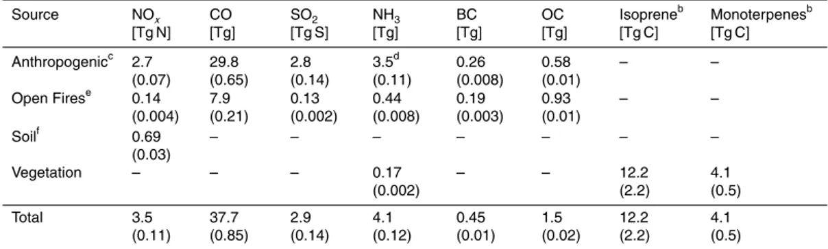
distribution of isoprene emissions. Total emissions over the Southeast US (domain

outlined in Fig. 2) during the 2 month SEAC

RS period were 2.2 Tg C for isoprene and

0.5 Tg C for monoterpenes. Monoterpene emissions did not exceed isoprene emission

anywhere.

Sulfate was too low in our initial simulations of the SEAC

RS observations. We

ad-5

dressed this problem by including SCIs as additional SO

oxidants in the model as

previously implemented in GEOS-Chem by Pierce et al. (2013). This significantly

re-duced the simulated mean bias and moderately improved the correlation with observed

sulfate in addition to providing a better representation of the SO

/

sulfate ratio (Sect. 4).

Oxidation of isoprene and monoterpenes provides a large source of SCIs in the

South-10

east US in summer. Sipila et al. (2014) estimated SCI molar yields from ozonolysis of

0.58

±

0.26 from isoprene, 0.15

±

0.07 from

α

-pinene, and 0.27

±

0.12 from limonene.

Sarwar et al. (2014) previously found that simulation of sulfate with the CMAQ CTM

compared better with summertime surface observations in the Southeast US when

SCI

₊

SO

reactions were included in the chemical mechanism. However, production

15

of sulfate from SCI chemistry may be severely limited by competition for SCIs between

SO

and water vapor and depends on the respective reaction rate constants (Welz

et al., 2012; Li et al., 2013; Newland et al., 2014; Sipila et al., 2014; Stone et al., 2014).

Here we use SCI chemistry from the Master Chemical Mechanism (MCMv3.2; Jenkins

et al., 1997; Saunders et al., 2003) with the SCI

₊

SO

and SCI

₊

H

O rate constants

20

from Stone et al. (2014), using CH

OO as a proxy for all SCIs, such that the SCI

₊

SO

pathway dominates. This would not be the case using the standard SCI

+

H

O and

sig-nificantly slower (

∼

1000

×

) SCI

+

SO

rate constants in MCM (Millet et al., 2015) or if

reaction with the water vapor dimer is important (Chao et al., 2015). Given these crude

approximations coupled with the uncertain SCI kinetics, the simulated SCI contribution

25

ACPD

Sources, seasonality,

and trends of

Southeast US aerosol

P. S. Kim et al.

Title Page

Abstract Introduction

Conclusions References

Tables Figures

◭ ◮

◭ ◮

Back Close

Full Screen / Esc

Printer-friendly Version Interactive Discussion

Discussion

P

a

per

|

Discussion

P

a

per

|

Discussion

P

a

per

|

Discussion

P

a

per

|

A number of mechanisms of varying complexity have been proposed to model OA

chemistry (Donahue et al., 2006; Henze et al., 2006; Ervens et al., 2011; Spracklen

et al., 2011; Murphy et al., 2012; Barsanti et al., 2013; Hermansson et al., 2014).

These mechanisms tend to be computationally expensive and appear to have only

lim-ited success in reproducing the observed variability of OA concentrations (Tsigaridis

5

et al., 2014). Here we use a simple linear approach to simulate five components of

OA – anthropogenic POA and SOA, open fire POA and SOA, and biogenic SOA.

Anthropogenic and open fire POA emissions are from the NEI08 and QFED2

inven-tories described above. For anthropogenic and open fire SOA, we adopt the Hodzic

and Jimenez (2011) empirical parameterization that assumes irreversible

condensa-10

tion of the oxidation products of VOC precursor gases (AVOC and BBVOC

respec-tively). AVOCs and BBVOCs are emitted in proportion to CO, with an emission

ra-tio of 0.069 g AVOC (g CO)

(Hayes et al., 2014) and 0.013 g BBVOC (g CO)

(Cubi-son et al., 2011). They are both oxidized by OH in the model with a rate constant of

1.25

_×

10

_cm

_molecule

_s

_{to generate SOA. This approach produces amounts of}

15

SOA and timescales of formation consistent with field measurements at many locations

(de Gouw and Jimenez, 2009; Hodzic and Jimenez, 2010; Cubison et al., 2011; Jolleys

et al., 2012; Hayes et al., 2014).

We assume biogenic SOA to be produced with a yield of 3 % from isoprene and 5 %

from monoterpenes, formed at the point of emission. Laboratory studies have shown

20

that di

_ff

erent biogenic SOA formation mechanisms operate depending on the NO

con-centration, which determines the fate of the organic peroxy radicals (RO

) produced

from VOC oxidation (Kroll et al., 2005, 2006; Chan et al., 2010; Xu et al., 2014). In the

high-NO regime the RO

radicals react with NO, while in the low-NO regime they react

with HO

, other RO

radicals, or isomerize. During SEAC

RS the two regimes were of

25

ACPD

Sources, seasonality,

and trends of

Southeast US aerosol

P. S. Kim et al.

Title Page

Abstract Introduction

Conclusions References

Tables Figures

◭ ◮

◭ ◮

Back Close

Full Screen / Esc

Printer-friendly Version Interactive Discussion

Discussion

P

a

per

|

Discussion

P

a

per

|

Discussion

P

a

per

|

Discussion

P

a

per

|

same in both pathways. The SOA is apportioned to the high- or low-NO tracer by the

fraction of RO

reacting with NO at the point and time of emission.

GEOS-Chem computes the AOD for each aerosol component

i

by summing the

optical depths over all vertical model layers

L

=

[1,

. . .

,

n

]:

AOD

=

X

i n

X

L=1

α

(

L

)

M

(

L

)

(1)

5

where

α

(

L

) and

M

(

L

) are respectively the component mass extinction e

ffi

ciency

(m

g

_{) and partial column mass (g m}

_{) for level}

_L

_{. The}

_α

i

values are pre-calculated

for selected wavelengths using a standard Mie scattering algorithm. The algorithm

as-sumes specified aerosol dry size distributions and optical properties from the Global

Aerosol Data Set (GADS; Koepke et al., 1997), with updates by Drury et al. (2010) on

10

the basis of summer observations from the ICARTT aircraft campaign over the

east-ern US. The mass extinction e

ffi

ciencies are then adjusted for hygroscopic growth as

a function of the local relative humidity (RH), following Martin et al. (2003). The total

AOD is reported here at 550 nm and is the sum of the contributions from all aerosol

components. Comparison of dry aerosol size distribution and hygroscopic growth show

15

good general agreement with observations similar to Drury et al. (2010) (Supplement).

Comparison of GEOS-FP ML heights with lidar and ceilometer data from SEAC

RS,

SOAS, and DISCOVER-AQ indicates a 30–50 % positive bias across the Southeast US

in daytime (Scarino et al., 2015; Millet et al., 2015). We decrease the daytime

GEOS-FP ML heights by 40 % in our simulation to correct for this bias. During SEAC

RS, ML

20

heights were measured by the NASA-Langley High Spectral Resolution Lidar (HSRL;

Hair et al., 2008). After correction, the modeled ML height is typically within 10 % of the

HSRL data along the SEAC

RS flight tracks, with a mean daytime value (

_±

1 standard

deviation) of 1690

±

440 m in the HSRL data and 1530

±

330 m in the model (Zhu et al.,

2015). The daytime ML was typically capped by a shallow cloud convective layer (CCL)

25

ACPD

Sources, seasonality,

and trends of

Southeast US aerosol

P. S. Kim et al.

Title Page

Abstract Introduction

Conclusions References

Tables Figures

◭ ◮

◭ ◮

Back Close

Full Screen / Esc

Printer-friendly Version Interactive Discussion

Discussion

P

a

per

|

Discussion

P

a

per

|

Discussion

P

a

per

|

Discussion

P

a

per

|

troposphere above. When giving column statistics we will refer to the ML as below

1.5 km and the CCL as between 1.5 and 3 km.

Several companion papers apply the same GEOS-Chem model configuration as

de-scribed here to other analyses of the SEAC

RS data focused on gas-phase chemistry.

These include investigation of the factors controlling ozone in the Southeast US (Travis

5

et al., 2015), isoprene chemistry and the formation of organic nitrates (Fisher et al.,

2015), validation of satellite HCHO data as constraints on isoprene emissions (Zhu

et al., 2015), and sensitivity to model grid resolution (Yu et al., 2015). These studies

include extensive comparisons to the gas-phase observations in SEAC

RS. Our focus

here will be on the aerosol observations.

10

3

Surface aerosol concentrations

We begin by evaluating the simulation of PM

and its components against ground

observations. Total PM

is measured gravimetrically at 35 % RH at a large number

of EPA monitoring sites (Fig. 3). Filter-based measurements of PM

composition are

taken every three days at surface networks including the EPA CSN (25 sites in the

15

study domain marked in Fig. 2, mostly in urban areas), IMPROVE (15 sites, mostly in

rural areas), and SEARCH (5 sites, urban and suburban/rural). These three networks

all provide 24 h average concentrations of the major ions (SNA), carbon species (BC

and OC), and dust, though there are di

ff

erences in protocols (Edgerton et al., 2005;

Hidy et al., 2014; Solomon et al., 2014), in particular with respect to OC artifact

correc-20

tion. The IMPROVE and SEARCH OC are both blank-corrected but in di

ff

erent ways

(Dillner et al., 2009; Chow et al., 2010), while CSN OC is uncorrected. We apply a

con-stant 0.3 µg m

_{background correction to the CSN OC data as in Hand et al. (2012b).}

The resulting CSN OC measurements are within 1 % of SEARCH and 44 % higher than

IMPROVE when averaged across the Southeast US. When necessary, OA is inferred

25

ACPD

Sources, seasonality,

and trends of

Southeast US aerosol

P. S. Kim et al.

Title Page

Abstract Introduction

Conclusions References

Tables Figures

◭ ◮

◭ ◮

Back Close

Full Screen / Esc

Printer-friendly Version Interactive Discussion

Discussion

P

a

per

|

Discussion

P

a

per

|

Discussion

P

a

per

|

Discussion

P

a

per

|

DC-8 aircraft (Sect. 4). We do not discuss sea-salt concentrations as they make a

neg-ligible contribution to PM

inland (

<

0.1 µg m

_{averaged across the EPA networks).}

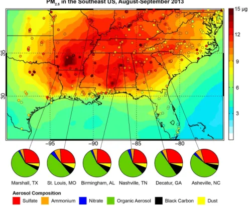
Figure 3 shows mean August–September 2013 PM

at the EPA sites and

com-pares to GEOS-Chem values. Concentrations peak over Arkansas, Louisiana, and

Mississippi, corresponding to the region of maximum isoprene emission in Fig. 2. The

5

spatial distribution and composition of PM

is otherwise fairly homogeneous across

the Southeast US, reflecting coherent stagnation, mixing, and ventilation of the region

(X. Zhang et al., 2012; Pfister et al., 2015). Sulfate accounts on average for 25 % of

PM

while OA accounts for 55 %. GEOS-Chem captures the broad features shown

in the surface station PM

data with little bias (

R

=

0.65, normalized mean bias or

10

NMB

₌

−

1.4 %). The model hotspot in southern Arkansas is due to OA from a

com-bination of biogenic emissions and agricultural fires. As discussed below, agricultural

fires make only a small contribution on a regional scale.

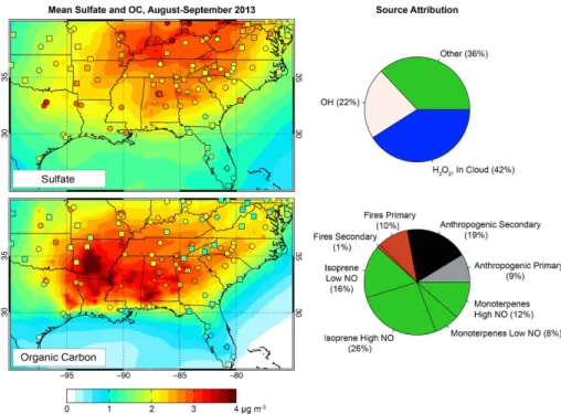
The spatial distributions of sulfate and OC concentrations are shown in Fig. 4. The

observed and simulated sulfate maxima are shifted to the northeast relative to total

15

PM

shown in Fig. 3. GEOS-Chem captures a larger fraction of the observed

vari-ability at rural sites (

R

=

0.78 for IMPROVE) than at urban/suburban sites (

R

=

0.71

for SEARCH, 0.62 for CSN) as would be expected from the sub-grid scale of urban

pollution. A scatterplot of the simulated daily mean surface sulfate concentrations

com-pared to the filter observations from all three networks in August–September 2013 is

20

shown in the Supplement. The model bias (NMB) is

₊

5 % relative to IMPROVE,

₊

10 %

relative to SEARCH, and

+

9 % relative to CSN. Over the Southeast US domain defined

in Fig. 2, 42 % of sulfate production is from in-cloud production by H

O

, 22 % is from

gas-phase oxidation by OH, and 36 % is from gas-phase oxidation by SCIs. Previous

studies by Pierce et al. (2013) and Boy et al. (2013) found similarly large contributions

25

ACPD

Sources, seasonality,

and trends of

Southeast US aerosol

P. S. Kim et al.

Title Page

Abstract Introduction

Conclusions References

Tables Figures

◭ ◮

◭ ◮

Back Close

Full Screen / Esc

Printer-friendly Version Interactive Discussion

Discussion

P

a

per

|

Discussion

P

a

per

|

Discussion

P

a

per

|

Discussion

P

a

per

|

The observed OC distribution shows a decreasing gradient from southwest to

north-east that maps onto the distribution of isoprene emissions shown in Fig. 2. The

IM-PROVE OC is generally low compared to CSN and SEARCH, as has been noted

pre-viously (Ford and Heald, 2013; Attwood et al., 2014). GEOS-Chem reproduces the

broad features of the observed OC distribution with moderate skill in capturing the

vari-5

ability (

R

=

0.64 for IMPROVE, 0.62 for SEARCH, 0.61 for CSN). Model OC is biased

high with a NMB of

+

66 % for IMPROVE,

+

29 % for SEARCH, and

+

14 % for CSN. The

range of NMBs for the di

_ff

erent networks could reflect di

_ff

erences in measurement

pro-tocols described above – IMPROVE OC is lower than SEARCH by 27 % for collocated

measurements made at Birmingham, Alabama (Supplement). We discuss this further

10

in the next section in the context of the aircraft data.

Source attribution of OC in the model (Fig. 4) suggests a dominance of biogenic

sources. Isoprene alone contributes 42 % of the regional OC burden. This is in

con-trast with previous work by Barsanti et al. (2013), who fitted chamber observations to

a model mechanism and found monoterpenes to be as or more important than

iso-15

prene as a source of OC in the Southeast US (particularly under low-NO conditions).

SEAC

RS observations of IEPOX-SOA (SOA formed from isoprene by the main

low-NO pathway) suggest that if anything the model underestimates the SOA yield from

isoprene (W. W. Hu et al., 2015; Campuzano-Jost et al., 2015; Liao et al., 2015).

Anthropogenic sources in the model contribute 28 % to regional OC, roughly evenly

20

distributed across the region. Open fires contribute 11 %, mainly from agricultural fires

in Arkansas and Missouri. Influence from western US fires was significant in the free

troposphere (see Sect. 4) but not at the surface.

When all of the components are taken together, we find that 81 % of the surface

OC in the Southeast US is secondary in origin. This is well above the 30–69 % range

25

ACPD

Sources, seasonality,

and trends of

Southeast US aerosol

P. S. Kim et al.

Title Page

Abstract Introduction

Conclusions References

Tables Figures

◭ ◮

◭ ◮

Back Close

Full Screen / Esc

Printer-friendly Version Interactive Discussion

Discussion

P

a

per

|

Discussion

P

a

per

|

Discussion

P

a

per

|

Discussion

P

a

per

|

primary and secondary OC respectively (Zotter et al., 2014; Hayes et al., 2014), we

estimate that 18 % of the total OC burden is derived from fossil fuel use. This is

consis-tent with an 18 % fossil fraction from radiocarbon measurements made on filter samples

collected in Alabama during SOAS (Edgerton et al., 2014).

4

Aerosol vertical profile

5

We now examine the aerosol vertical distribution measured by the NASA DC-8 aircraft

and simulated by GEOS-Chem along the flight tracks on 18 flights over the Southeast

US (Fig. 2). Aerosol mass composition was measured by a High-Resolution Aerodyne

AMS for SNA and OA (Canagaratna et al., 2007) and by the NOAA humidified dual

single-particle soot photometer for BC (HD-SP2; Schwarz et al., 2015). Dust

concentra-10

tions can be inferred from filter samples (Dibb et al., 2003), but the ML values are

_∼

10

_×

higher than measured by surface networks or simulated in GEOS-Chem, as previously

found by Drury et al. (2010) during ICARTT. Instead we estimate dust concentrations

from Particle Analysis by Laser Mass Spectrometer (PALMS) measurements (Thomson

et al., 2000; Murphy et al., 2006). The PALMS data provide the size-resolved number

15

fraction of dust-containing particles, which is multiplied by the measured aerosol

vol-ume size distribution from the LAS instrvol-ument (Thornhill et al., 2008; Chen et al., 2011)

and an assumed density of 2.5 g cm

. The size distribution is truncated to PM

by

applying the transmission curve for the 2.5 µm aerosol impactor used by the ground

networks.

20

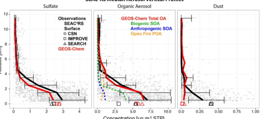
Figure 5 shows the median sulfate, OA, and dust vertical profiles over the

South-east US. Also shown are the median concentrations from the surface networks over

the study domain shown in Fig. 2. The di

_ff

erence between the surface and aircraft data

that can be attributed to di

_ff

erences in sampling (time and duration) is quantified by

the di

ff

erence in GEOS-Chem output when the model is sampled with the surface data

25

ACPD

Sources, seasonality,

and trends of

Southeast US aerosol

P. S. Kim et al.

Title Page

Abstract Introduction

Conclusions References

Tables Figures

◭ ◮

◭ ◮

Back Close

Full Screen / Esc

Printer-friendly Version Interactive Discussion

Discussion

P

a

per

|

Discussion

P

a

per

|

Discussion

P

a

per

|

Discussion

P

a

per

|

observations by 5–10 % as discussed in Sect. 3; these small inconsistent biases may

not be significant. The general shape of the vertical profile is well simulated (with a low

bias from 3 to 4 km) and this applies also to SO

and to the SO

/

sulfate ratio

(Supple-ment). The sulfate concentrations are highest near the surface and drop rapidly with

altitude, but there is significant mass loading in the lower free troposphere. 23 % of

5

the observed sulfate column mass lies in the free troposphere above 3 km and this is

well simulated by the model (23 %). Analysis of SENEX and SEAC

RS vertical

pro-files by Wagner et al. (2015) suggests that most of this free tropospheric sulfate is

ventilated from the PBL rather than being produced within the free troposphere from

ventilated SO

. GEOS-Chem shows moderate skill in explaining the variability in the

10

aircraft sulfate data (

R

=

0.81 for all observations in the Southeast US,

R

=

0.68 below

3 km,

R

=

0.49 above 3 km).

Similarly to sulfate, OA measured from aircraft peaks at the surface and decreases

rapidly with height (Fig. 5). The aircraft OA mass concentration below 1 km is 25–

50 % higher than measured at the surface networks. IMPROVE is substantially lower

15

than the other networks, as has been noted above and in previous studies (Ford and

Heald, 2013; Attwood et al., 2014), and may be due to instrumental issues particular to

that network. The discrepancy between the AMS observations and CSN/SEARCH can

largely be explained by di

ff

erences in sampling, as shown by the model. The

GEOS-Chem simulation matches closely the aircraft observations while being 14–66 % higher

20

than the surface networks as reported above. The vertical distribution of OA is similar

to that of sulfate, with 20 % of the total column being above 3 km both in the model

and in the observations. The GEOS-Chem source attribution, also shown in Fig. 5,

indicates that open fires contribute

_∼

50 % of OA in the free troposphere. This fire

influence is seen in the observations as occasional plumes of OA up to 6–7 km altitude

25

ACPD

Sources, seasonality,

and trends of

Southeast US aerosol

P. S. Kim et al.

Title Page

Abstract Introduction

Conclusions References

Tables Figures

◭ ◮

◭ ◮

Back Close

Full Screen / Esc

Printer-friendly Version Interactive Discussion

Discussion

P

a

per

|

Discussion

P

a

per

|

Discussion

P

a

per

|

Discussion

P

a

per

|

the model does require buoyant injection of western US wildfire emissions in the free

troposphere, as noted in previous studies (Turquety et al., 2007; Fischer et al., 2014).

Comparison of GEOS-Chem to the individual OA observations along the aircraft flight

tracks shows good simulation of the variability (

R

=

0.82 for all observations,

R

=

0.74

below 3 km,

R

=

0.42 above 3 km). This is despite (or maybe because of) our use

5

of a very simple parameterization for the OA source. The successful GEOS-Chem

simulation of the OA vertical profile argues against a large CCL source from

aqueous-phase cloud processing. This is supported by the work of Wagner et al. (2015), who

found little OA enhancement in air masses processed by cumulus wet convection.

Dust made only a minor contribution to total aerosol mass in the Southeast US

dur-10

ing SEAC

RS, accounting for less than 10 % of observed surface PM

(Fig. 3). The

PBL dust concentrations measured by PALMS are roughly consistent with the surface

data but the model is much lower (Fig. 5). This reflects a southward bias in the model

transport of Saharan dust (Fairlie et al., 2007), but is of little consequence for the

sim-ulation of PM

or the AOD

/

PM relationship over the Southeast US. Figure 5 shows

15

few free tropospheric plumes in the SEAC

RS observations, consistent with the dust

climatology compiled from CALIOP data by Liu et al. (2008).

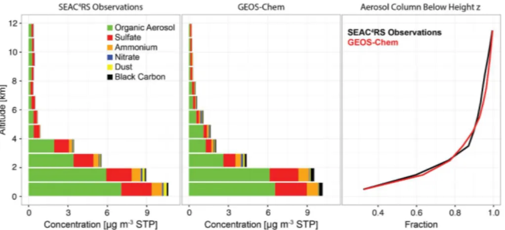
Figure 6 compiles the median observed and simulated vertical profiles of aerosol

concentrations and composition during SEAC

RS. OA and sulfate dominate at all

al-titudes. Ammonium is associated with sulfate as discussed in the next Section. OA

20

accounts for most of PM

below 1 km, with a mass fraction

F

=

[OA]

/

[PM

] of

0.66 g g

_{(0.65 in GEOS-Chem). This is consistent with the surface SEARCH data}

(

F

=

0.56 g g

_{). Figure 1 shows a lower}

_F

OA

in the IMPROVE surface observations,

increasing from 0.34 g g

in 2003 to 0.44 g g

in 2013, reflecting instrumentation bias

as discussed above. The aircraft data show that most of the aerosol mass is OA at

25

ACPD

Sources, seasonality,

and trends of

Southeast US aerosol

P. S. Kim et al.

Title Page

Abstract Introduction

Conclusions References

Tables Figures

◭ ◮

◭ ◮

Back Close

Full Screen / Esc

Printer-friendly Version Interactive Discussion

Discussion

P

a

per

|

Discussion

P

a

per

|

Discussion

P

a

per

|

Discussion

P

a

per

|

aerosol mass, and this is an important result for application of the model to derive the

AOD

/

PM relationship.

5

Extent of neutralization of sulfate aerosol

The extent of neutralization of sulfate aerosol by ammonia, computed from the fraction

f

=

[NH

]

/

(2[SO

4

]

+

[NO

−

3

]) where concentrations are molar, has important

implica-5

tions for the aerosol phase and hygroscopicity, for the formation of aerosol nitrate

(Mar-tin et al., 2004; Wang et al., 2008), and for the formation of SOA (Froyd et al., 2010;

Eddingsaas et al., 2012; McNeill et al., 2012; Budisulistiorini et al., 2013; Liao et al.,

2015). Figure 6 shows ammonium to be the third most important aerosol component

by mass in the Southeast US in summer after OA and sulfate. Summertime

particle-10

phase ammonium concentrations have declined at approximately the same rate as

sulfate from 2003 to 2013 (Fig. 1 and Blanchard et al., 2013). However, we find no

significant trend over that time in ammonium wet deposition fluxes over the Southeast

US (National Atmospheric Deposition Program, 2015), in contrast to a

_∼

50 % decline

in sulfate wet deposition. This implies that ammonia emissions have not decreased but

15

the partitioning into the aerosol has.

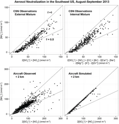
One would expect ammonium aerosol trends to follow those of sulfate if the aerosol is

fully neutralized (

f

=

1), so that partitioning of ammonia into the aerosol phase is limited

by the supply of sulfate. However, this is not the case in the observations. Figure 7

shows the extent of neutralization in the observations and the model assuming that the

20

SNA aerosol is externally mixed from other ionic aerosol components such as dust. The

model aerosol is fully neutralized (

f

=

1) but the observed aerosol is not, with a median

extent of neutralization of 0.55 mol mol

_{in the CSN data and 0.68 mol mol}

_{in the}

AMS data below 2 km. This is comparable to

f

=

0.49 mol mol

_{observed at the SOAS}

Centreville site earlier in the summer. The CSN data include full ionic analysis and we

25

ACPD

Sources, seasonality,

and trends of

Southeast US aerosol

P. S. Kim et al.

Title Page

Abstract Introduction

Conclusions References

Tables Figures

◭ ◮

◭ ◮

Back Close

Full Screen / Esc

Printer-friendly Version Interactive Discussion

Discussion

P

a

per

|

Discussion

P

a

per

|

Discussion

P

a

per

|

Discussion

P

a

per

|

concentrations of these other ions. The AMS reports total sulfate. While organosulfates

have a low pKa and would interact with ammonium as a single charged ion, they were

typically a small fraction of total sulfate (Liao et al., 2015).

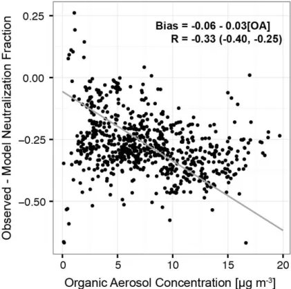
A possible explanation is that ammonia uptake by aerosol with

f <

1 may be inhibited

by organic particle material. This has been demonstrated in a laboratory study by

Lig-5

gio et al. (2011), who show that the time constant for ammonia to be taken up by sulfate

aerosol with incomplete extent of neutralization increases with the ratio of condensing

organic gases to sulfate and may be hours to days. We tested this hypothesis by

ex-amining the relationship between the model neutralization bias (the di

ff

erence between

simulated and observed

f

) and the OA concentration in the aircraft observations

be-10

low 1 km, assuming sulfate and OA to be internally mixed (consistent with the PALMS

observations). We find a significant correlation (

R

=

−

0.33, with a bootstrapped 95 %

confidence interval of [

−

0.40,

−

0.25]) as shown in Fig. 8, which provides some support

for organic-driven inhibition of ammonia uptake by sulfate aerosol.

The complete extent of neutralization of sulfate aerosol in the model, in contrast to

15

the observations, leads to bias in the simulated aerosol phase and hygroscopicity for

relating AOD to PM. Calculations by Wang et al. (2008) for ammonium-sulfate particles

of di

_ff

erent compositions show a 10–20 % sensitivity of the mass extinction e

_ffi

ciency

to the extent of neutralization, with the e

ff

ect changing sign depending on composition

and RH. An additional e

_ff

ect of

f

=

1 in the model would be to allow formation of

am-20

monium nitrate aerosol, but nitrate aerosol is negligibly small in the model as it is in the

observations (Fig. 6). At the high temperatures over the Southeast US in the summer,

we find in the model that the product of HNO

and NH

partial pressures is

gener-ally below the equilibrium constant for formation of nitrate aerosol. By contrast, surface

network observations in winter show nitrate to be a large component of surface PM

25

ACPD

Sources, seasonality,

and trends of

Southeast US aerosol

P. S. Kim et al.

Title Page

Abstract Introduction

Conclusions References

Tables Figures

◭ ◮

◭ ◮

Back Close

Full Screen / Esc

Printer-friendly Version Interactive Discussion

Discussion

P

a

per

|

Discussion

P

a

per

|

Discussion

P

a

per

|

Discussion

P

a

per

|

6

Aerosol extinction and optical depth

We turn next to light extinction measurements onboard the DC-8 to better

under-stand the relationship between the vertical profiles of aerosol mass (Sect. 4) and AOD.

Aerosol extinction coe

_ffi

cients were measured on the SEAC

RS aircraft remotely above

and below the aircraft by the NASA HSRL and at the altitude of the aircraft by the in

5

situ NOAA cavity ringdown spectrometer (CRDS; Langridge et al., 2011). Figure 9

compares the two measurements, both at 532 nm, with GEOS-Chem. Though the two

instruments sampled di

_ff

erent regions of the atmosphere at any given time, the

mis-sion median profiles are similar. The exception is between 2 and 4 km where the HSRL

extinction coe

ffi

cient is lower. The shapes of the vertical extinction profiles are

consis-10

tent with aerosol mass (Fig. 6). The fraction of total column aerosol extinction below

3 km is 93 % for the HSRL data (91 % in GEOS-Chem when sampled at the

obser-vation times) and 85 % for the CRDS data (85 % in GEOS-Chem). The atmosphere

below 3 km contributes more to total aerosol extinction than to aerosol mass (80 %,

see Sect. 4) because of higher RH and hence hygroscopic growth of particles. Almost

15

all of the column extinction is below 5 km (94 % for the CRDS and 93 % for

GEOS-Chem). Integrated up to the ceiling of the DC-8 aircraft, the median AODs from HSRL

and the CRDS are 0.14 and 0.17 respectively (0.12 and 0.15 for GEOS-Chem).

Figure 10 shows maps of the mean AOD over the Southeast US in August–

September 2013 as measured by AERONET, MISR, MODIS on the Aqua satellite,

20

and simulated by GEOS-Chem. The model is sampled at the local satellite overpass

times (10:30 for MISR and 13:30 for MODIS). We use the Version 31 Level 3 product

from MISR (gridded averages at 0.5

×

0.5

resolution) and the Collection 6 Level 3

product from MODIS (gridded averages at 1

×

1

resolution). We exclude MODIS

ob-servations with cloud fraction greater than 0.5 or AOD greater than 1.5 to account for

25

ACPD

Sources, seasonality,

and trends of

Southeast US aerosol

P. S. Kim et al.

Title Page

Abstract Introduction

Conclusions References

Tables Figures

◭ ◮

◭ ◮

Back Close

Full Screen / Esc

Printer-friendly Version Interactive Discussion

Discussion

P

a

per

|

Discussion

P

a

per

|

Discussion

P

a

per

|

Discussion

P

a

per

|

Comparison of daily collocated MODIS and MISR retrievals with AERONET

obser-vations shows high correlation and little bias (statistics inset in Fig. 10). MODIS shows

a broad maximum over the Southeast US that corresponds well with observed PM

in Fig. 3. There is greater heterogeneity in the MISR average due to sparse sampling.

GEOS-Chem captures the spatial pattern of the regional AOD enhancement when

5

sampled with the di

ff

erent retrievals and underestimates the magnitude by 16 % (NMB

relative to AERONET), consistent with the underestimate of the aircraft aerosol

extinc-tion data.

7

The aerosol seasonal cycle

As pointed out in the introduction, there has been considerable interest in interpreting

10

the aerosol seasonal cycle over the Southeast US and the di

_ff

erence in seasonal

am-plitude between AOD and surface PM

(Goldstein et al., 2009; Ford and Heald, 2013).

Figure 11 shows MODIS monthly average AOD over the Southeast US for 2006–2013.

The observed AOD in 2013 shows a seasonal cycle consistent with previous years.

There has been a general decline in the seasonal amplitude over 2006–2013 driven

15

by a negative summertime trend, with 2011 being anomalous due to high fire

activ-ity (NOAA, 2011). The same long-term decrease and 2011 anomaly are seen in the

surface PM

data (Fig. 1). Examination of Fig. 11 reveals that the entirety of the

seasonal decrease from summer to winter takes place as a sharp transition in the

August–October window, in all years.

20

We analyzed the causes of this August–October transition using the GEOS-Chem

simulation of the SEAC

RS period. Figure 12a shows the time series of daily

me-dian AOD from AERONET, GEOS-Chem sampled at the times and locations of the

AERONET observations, and MODIS over the Southeast US. The di

_ff

erence between

AERONET and MODIS can be explained by di

ff

erences in sampling (they otherwise

25

ACPD

Sources, seasonality,

and trends of

Southeast US aerosol

P. S. Kim et al.

Title Page

Abstract Introduction

Conclusions References

Tables Figures

◭ ◮

◭ ◮

Back Close

Full Screen / Esc

Printer-friendly Version Interactive Discussion

Discussion

P

a

per

|

Discussion

P

a

per

|

Discussion

P

a

per

|

Discussion

P

a

per

|

well reproduced by the model. The observed AODs then fall sharply in mid-September

and again this is well reproduced by GEOS-Chem. The successful simulation of the

August–October seasonal transition implies that we can use the model to understand

the causes of this transition. Figure 12 also shows the sulfate and OA contributions to

GEOS-Chem AOD. Sulfate aerosol contributes as much to column light extinction as

5

OA, despite lower concentrations, due to its higher mass extinction e

ffi

ciency. Both the

sulfate and OA contributions to AOD fall during the seasonal transition.

We find that the sharp drops in sulfate and OA concentrations over August–October

are due to two factors. The first is a decline in isoprene and monoterpene emissions

due to cooler surface temperatures and leaf senescence (Fig. 12b). The second is

10

a transition in the photochemical regime as UV radiation sharply declines (Kleinman,

1991; Jacob et al., 1995), depleting OH and H

O

(Fig. 12c) and hence sulfate

forma-tion.

The seasonal transition in photochemical regime also involves a shift from a low-NO

to a high-NO chemical regime (Kleinman, 1991; Jacob et al., 1995). This would a

_ff

ect

15

the SOA yield (Marais et al., 2015). Figure 12d shows the ratio of isoprene

hydroper-oxides (ISOPOOH) to isoprene nitrate (ISOPN) concentrations measured in the PBL

during SEAC

RS by the Caltech CIMS (Crounse et al., 2006; St. Clair et al., 2010)

and simulated by GEOS-Chem. ISOPOOH is formed under low-NO conditions, while

ISOPN is formed under high-NO conditions. Both observations and the model show

20

a decline in the ISOPOOH

/

ISOPN concentration ratio over the course of SEAC

RS,

with the model showing extended decline into October. If the SOA yield is higher

un-der low-NO conditions (Kroll et al., 2005, 2006; Xu et al., 2014) then this would also

contribute to the seasonal decline in OA.

We have thus explained the seasonality of AOD as driven by aerosol sources.

Previ-25

ACPD

Sources, seasonality,

and trends of

Southeast US aerosol

P. S. Kim et al.

Title Page

Abstract Introduction

Conclusions References

Tables Figures

◭ ◮

◭ ◮

Back Close

Full Screen / Esc

Printer-friendly Version Interactive Discussion

Discussion

P

a

per

|

Discussion

P

a

per

|

Discussion

P

a

per

|

Discussion

P

a

per

|

by the seasonal variation in ML height (middle panel of Fig. 13), dampening the

sea-sonal cycle of PM

by reducing ventilation in winter. The AOD in GEOS-Chem is lower

than observed in summer and higher in winter, so that the seasonality is weaker than

observed. The summer underestimate is consistent with the aircraft observations, as

discussed previously. The winter overestimate could reflect seasonal error in model

5

aerosol sources or optical properties.

8

Conclusions

We have used a large ensemble of surface, aircraft, and satellite observations during

the SEAC

RS field campaign over the Southeast US in August–September 2013 to

better understand (1) the sources of sulfate and organic aerosol (OA) in the region,

10

(2) the relationship between the aerosol optical depth (AOD) measured from space

and the fine particulate matter concentration (PM

) measured at the surface; and (3)

the seasonal aerosol cycle and the apparent inconsistency between satellite and

sur-face measurements. Our work used the GEOS-Chem global chemical transport model

(CTM) with 0.25

×

0.3125

(

∼

25 km

×

25 km) horizontal resolution over North America

15

as an integrative platform to compare and interpret the ensemble of observations.

PM

surface observations are fairly homogenous across the Southeast US,

reflect-ing regional coherence in stagnation, mixreflect-ing, and ventilation. Sulfate and OA account

for the bulk of PM

. GEOS-Chem simulates sulfate without bias but this requires

un-certain consideration of SO

oxidation by stabilized Criegee intermediates to account

20

for 30 % of sulfate production. The OA simulation bias is

+

14 % relative to CSN sites

and

+

66 % relative to IMPROVE sites but the IMPROVE data may be too low. OA in

the model originates from biogenic isoprene (40 %) and monoterpenes (20 %),

anthro-pogenic sources (30 %) and open fires (10 %).

Aircraft vertical profiles show that 60 % of the aerosol column mass is in the mixed

25