The effect of a localized geothermal heat source on deep water formation

www.nonlin-processes-geophys.net/18/841/2011/ doi:10.5194/npg-18-841-2011

© Author(s) 2011. CC Attribution 3.0 License.

in Geophysics

The effect of a localized geothermal heat source on deep

water formation

M. Vincze, A. V´arai, E. Barsy, and I. M. J´anosi

von K´arm´an Laboratory for Environmental Flows, E¨otv¨os Lor´and University, P´azm´any P. s. 1/A, 1117 Budapest, Hungary Received: 3 August 2011 – Revised: 27 October 2011 – Accepted: 10 November 2011 – Published: 17 November 2011

Abstract. In a simplified two-dimensional model of a buoyancy-driven overturning circulation, we numerically study the response of the flow to a small localized heat source at the bottom. The flow is driven by differential thermal forc-ing applied along the top surface boundary. We evaluate the steady state solutions versus the temperature difference be-tween the two ends of the water surface in terms of different characteristic parameters that properly describe the transition from a weak upper-layer convection state to a robust full-depth deep convection. We conclude that a small additional bottom heat flux underneath the “cold” end of the basin is able to initiate full-depth convection even when the surface heat forcing alone is not sufficient to maintain this state.

1 Introduction

The engine of the Great Ocean Conveyor is the sinking of cold and saline surface waters to the bottom of the oceanic basin, referred to as Deep Water Formation (DWF). Under the present climatic conditions, DWF can occur only at a few compact polar downwelling regions, all of which are located in the Atlantic basin (van Aken, 2007). This polar sinking to-gether with the distributed upwelling of water masses drives the Atlantic Meridional Overturning Circulation (AMOC) (Stommel, 1958), which is an important contributor to the European climate, because of its large northward heat trans-port of an order of magnitude of 1015W (Ganachaud and Wunsch, 2000).

The question arises of what makes the Atlantic the only basin where DWF can occur among the present climatic con-ditions. The average surface salinity of the Atlantic is signif-icantly higher than that of all other basins, due to its larger

Correspondence to:M. Vincze (vincze.m@lecso.elte.hu)

evaporation-precipitation difference. The combined effect of high salinity and the heat release, which occurs in the po-lar regions results in an unstable stratification that makes the dense surface water parcels descend to the bottom. However, it has been shown that the amount of precipitation is quite similar over the Atlantic and the Pacific, and the evaporation difference is due to the temperature difference between the basins, which is largely a consequence of the ocean circula-tion itself (Huisman et al., 2009). This implies that the cor-rect explanation of the Atlantic DWF must involve additional effects besides the widely studied role of surface buoyancy (i.e. heat or fresh water) fluxes.

pact, localized bottom heat source, placed underneath the “polar” end of the basin, where the surface heat flow is neg-ative (cooling occurs).

Although the concept originates from the above discussed oceanographic problem, the parameters used here are rather unrealistic, as we intended to model a laboratory-scale setup for a better understanding of the basic underlying physics. Furthermore, we think that such parametrization supports a direct comparison with actual experiments (we compare some aspects of the ocean circulation and the numerical and experimental setups in the Appendices). Our main result is that even a weak local heat source beneath the cold end of the basin perturbs significantly the initially shallow-layer hori-zontal convection and markedly contributes to the DWF pro-cess.

2 The model setup and numerical methods

The present model is based on the two-dimensional non-hydrostatic Boussinesq equations. These were solved on a 20_×200 equidistant array of Arakawa C cells (Arakawa and Lamb, 1977) which corresponds to a 2 m deep and 20 m long rectangular tank. The effect of salinity differences was not considered, hence the flow was only forced by the in-coming heat fluxes from the surface, the bottom and the lateral sidewalls (a qualitative argument on the possible ef-fect of salinity on the phenomena described here, is pre-sented in Appendix B). The densityρ(T ) was assumed to obey a linear temperature dependence with reference val-uesTref=25◦C,ρref=997.075 kg m−3and volumetric ther-mal expansion coefficientα₌2.5×10−4 K−1. The kine-matic viscosityν₌10−6m2s−1and the thermal diffusivity κ₌1.4·10−7m2s−1were treated as isotropic constants, of their usual molecular values, resulting in a Prandtl number of P r₌7.14. We note, that the three orders of magnitude larger eddy viscosity and diffusivity values that are set in ocean models (e.g.νeddy∼10−3m2s−1 andκeddy∼10−4m2s−1, as in Frankcombe et al. (2009)) yield approximately the same dimensionless ratio, therefore this part of the dynamics re-mains unchanged by the upscaling.

Numerical solutions were obtained using the Advanced Ocean Modeling open-source software package, written in FORTRAN95 environment (K¨ampf, 2009), in which the sys-tem of PDEs are being solved with the Successive Over-Relaxation (SOR) method.

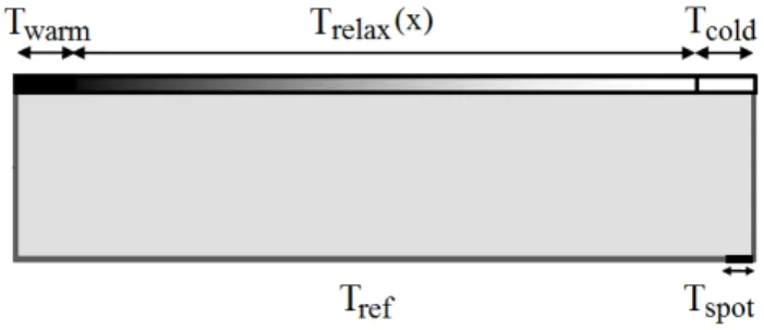
Fig. 1.The schematic drawing of the setup, with the domains where the different values ofTrelaxwere applied along the boundaries.

According to the initial conditions, the fluid was at rest and its temperature was uniformly set to the value of Tref in the whole solution domain. At the water surface and the sidewalls slip boundary conditions were applied for the ve-locities, while friction was taken into account at the bottom in the form of

ν∂u ∂z

bottom

=rub|ub|, (1)

whereudenotes the horizontal velocity, with a value ofub

adjacent to the bottom boundary, and the bottom-drag coef-ficient r was set to 0.001 as by K¨ampf (2009). The flows in the domain were forced by restoring temperature bound-ary conditions at all boundaries, represented by a distributed heat source that is proportional to the temperature difference between the local water temperature and a spatially varying prescribed temperature fieldTrelax(x,z), as given by:

∂T

∂t = − 1

τ(T−Trelax). (2)

Generally, the restoring timescaleτ was set to 2100 s at all boundaries, based on our laboratory measurements (details will be reported elsewhere). We note here, that for an ex-tension of a similar model setup to oceanic scales one can-not apply the same restoring timescales at the water surface and at the other boundaries. In the case of a real ocean the heat exchange between the uppermost layer and the atmo-sphere is orders of magnitude more effective (τ ∼30 days, as in Frankcombe et al. (2009)) than it is at the abyssal re-gions, due to the wind-driven turbulent mixing. However, for a laboratory-scale setup that is studied here the usage of the same restoring timescales at all boundaries is a reason-able assumption. Further comparison of the thermal bound-ary conditions of the setup and the ocean can be found in Appendix A.

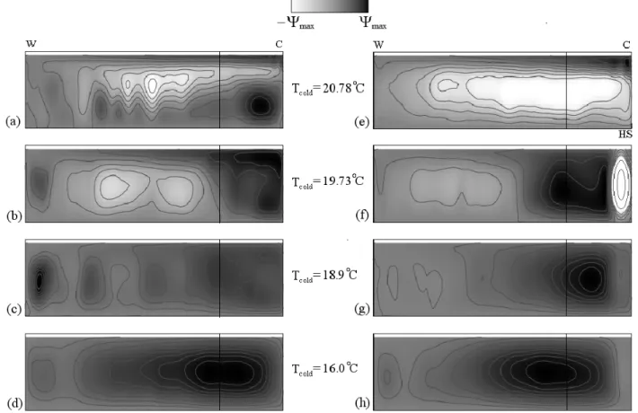
Fig. 2.Averaged streamfunction (9) patterns for the quasi-stationary parts of different runs. The gray-scale values cover the interval between

−9max(white) and9max(black), for actual magnitudes see Fig. 3c and f. Correspondingly, dark gray regions reflect positive (clockwise) local vorticity. In the uppermost two snapshots, labels “W” and “C” denote the warming and cooling sides. Label “HS” marks the position of the bottom “hot spot”. Figures 2a,b,c and d correspond to the “no hot spot” scenario, i.e.Tspot=Tref=25◦C. The transition from a multi-cellular weak convection state to a DWF state is clearly visible as a function ofTcold. In Fig. 2e,f,g and h the same transition is shown in the case ofTspot=30◦C. In Fig. 2e the presence of the hot spot initiates a marked two-cell convection along the whole basin, which – atTcold=19.73◦C – develops to a full-depth counterclockwise Benard cell above the hot spot (Fig. 2f), that transfers momentum to the neighboring anticyclonic downwelling. In Fig. 2g the full-depth DWF state is present, and the counterclockwise cell already vanished. Note, that in the “hot spot” case, the marked one-cell convection is visible atTcold=18.9◦C, unlike in the “no hot spot” case. The vertical lines in each snapshot represent the left boundary of the region over which the mean valuehwipolar(see Fig. 3b and e) is evaluated.

ofTcold=4–24◦C for the different numerical experiments. Between these sections – that model the equatorial and polar regions of the ocean surface – the value of the restoring tem-perature was interpolated linearly betweenTwarmandTcoldat the water surface, as depicted in Fig. 1.

Besides Tcold, our other key control parameter was the restoring temperatureTrelax(x,z)₌Tspotof a “hot spot”, i.e. a 10 parcel-long section at the bottom right corner of the basin (see Fig. 1). This domain represents the aforementioned compact Atlantic seafloor regions of high geothermal flux at higher latitudes. Tspot varied in an interval between 25◦C (₌Tref) and 35◦C for the different runs.

The spin-up time of the model was taken to be 12 000 s, after which a quasi-stationarity of the average surface tem-perature time series was achieved in every run. In order to properly describe the transition between the different

con-vection states, we introduced some characteristic parameters, which exhibit jumps at the transitions between different dy-namical regimes. These parameters were evaluated for the quasi-stationary part of the process.

3 Results

24.5

24.5

-0.003

-0.002

-0.001

0

<w> polar

[m/s]

-0.003

-0.002

-0.001

0

12.5

15

17.5

20

22.5

T_cold [oC]

0

0.01

0.02

0.03

Ψ_max

[m2/s]

12.5

15

17.5

20

22.5

T_cold [oC]

0

0.01

0.02

0.03

(a)

(b)

(c)

(d)

(e)

(f)

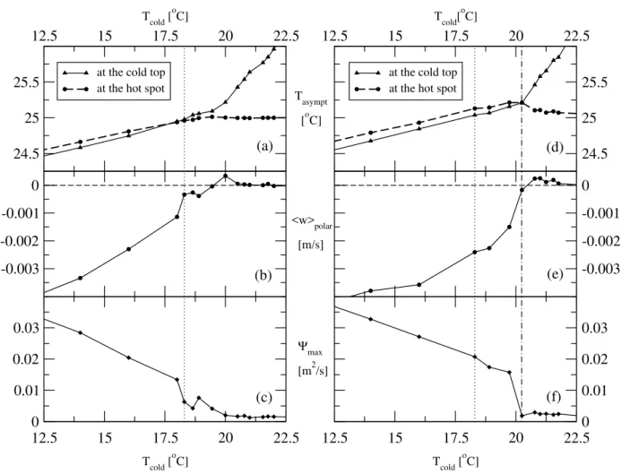
Fig. 3.TheTcolddependence of three parameters that characterize the transition between the convection states. As in Fig. 2, the left column corresponds to the “no hot spot” scenario, and the right column shows theTspot=30◦C case. Figures 3a and d represent the quasi-equilibrium temperatures at the right (cold) margin of the basin at the surface and at the bottom. Figures 3b and e depict the vertical velocity (hwipolar) averaged over the region that is indicated in Fig. 2. The maxima of the streamfunctions (9max) are shown in Figs. 3c and f. The dashed and dashed-dotted vertical lines mark the criticalTcold, where the onset of DWF takes place in the “no hot spot” and in the “hot spot” case, respectively.

Naturally, the onset of DWF is related to the presence of unstable density stratification at the “polar” region of the tank. Firstly, we determined the time averaged temperatures T_asympttop andT_asymptbottom, measured at the rightmost upper and bot-tom corners of the basin (solid and dashed lines with symbols in Fig. 3a). It is clearly visible in the higherTcold-range that the asymptotic bottom temperature practically reaches the prescribed value ofTref₌25◦C. This implies that the bottom layer of the fluid stays at rest in this regime. The transition – whereTasymptreaches the same value at the surface and at the bottom – occurs atT∗

cold=18.3◦C (denoted with dotted vertical line in Fig. 3a, b and c).

Next, we measured the mean vertical sinking velocity hw_{ipolar, that is averaged in the 5 m long “polar” section} identified by the vertical lines in Fig. 2. (Negative values ofhw_ipolarrepresent downward flow.) The onset of DWF is

clearly indicated as a break point atT_cold∗ ₌18.3◦C (Fig. 3b). At temperature valuesTcold< Tcold∗ , the mean vertical veloc-itieshw_ipolarhave definite negative values.

Thirdly, we computed the maximal value of the time-averaged streamfunction (9max) for each run. The curve in Fig. 3c demonstrates the same transition: in the range Tcold< Tcold∗ , the large values of9maxare related to vigor-ous deep-water convection.

10 12 14 16 18 20 22 T

cold [ o

C]

-0.005 -0.004 -0.003 -0.002 -0.001 0

<w>

polar

[m/s]

T_spot = 25oC

T

spot = 27.5

o

C

T_spot = 30oC

T_spot = 32.5oC

24 26 28 30 32 34 36

T

spot [ o

C] -0.0025

-0.002 -0.0015 -0.001 -0.0005 0

T_cold = 20.78oC

T_cold = 19.73oC

T

cold = 18.9

o

C

(a)

_(b)

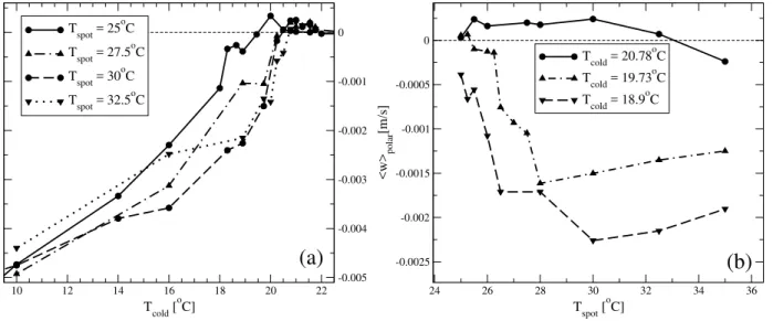
Fig. 4.(a)hwipolaras a function ofTcold, for four different values ofTspot, see legends. (b) Dependence of the same quantityhwipolaron

Tspot, for three fixed values ofTcold, see legends.

the presence of the additional “geothermal heat”, the critical value ofT_cold∗ has shifted considerably upward, to the value of 20.2◦C (dashed-dotted in the right column of Fig. 3).

The next question of importance is whether there exists a certainTspot for a givenTcold that maximizes the flux of the polar downwelling. Intuitively, one can argue that over a certain temperature threshold the bottom hot spot launches a rising plume – as discussed in e.g.: Stommel (1982) – that would tend to reverse the direction of the circulation, thus hindering DWF rather than enhancing it. Fig. 4a shows hw_ipolar as a function ofTcold for Tspot=25.0, 27.2, 30.0, and 32.5◦C, the first and third curve being the same as in Figs. 3b and e. There are two main observations to be empha-sized: firstly, the critical crossover temperatureT_cold∗ depends weakly on the restoring hot spot temperatureTspot; secondly, the largest downward flux values in the rangeTcold< T_cold∗ do not belong to the highest value ofTspot. According to the expectations, high enoughTspottemperatures seem to hinder DWF, see the dotted line in Fig. 4a, in the range ofTcold< 15◦_{C (forTspot=32.5}◦_C).

In order to move along an orthogonal axis of the parame-ter space, we evaluated the same quantityhw_ipolaras a func-tion of the bottom heating in a broaderTspotrange for three fixedTcoldvalues (Fig. 4b). When the driving horizontal tem-perature differenceTwarm−Tcoldis too small, DWF is hin-dered even when some hot spot is present (see the topmost curve of Fig. 4b,Twarm₌32.00◦C as in each case,Tcold₌ 20.78◦C). At large enough horizontal temperature gradients, a localized bottom heat source enhances downward DWF fluxes, exhibiting an optimal value atT_spotopt₌28◦C forTcold₌ 19.73◦C (middle curve in Fig. 4b), and T_spotopt ₌ 30◦C for Tcold₌18.90◦C (lowermost curve in Fig. 4b). Both series

of experiments point out that – in agreement with the quali-tative reasoning – there exists a small value of localized heat flux for every given “equator-to-pole” temperature difference that is capable to maximize the flux rate of DWF.

4 Conclusions

We performed numerical experiments in a simplified, two-dimensional laboratory-scale setup in order to capture the basic effects of a localized bottom heat source on Deep Wa-ter Formation in a convective system driven basically by top heat fluxes. As far as we know, this is the first study in a similar arrangement. Previous studies, such as Mullarney et al. (2006) incorporateduniform bottom heatingand pointed out strong perturbations in the convection, however they did not study an isolated heat source. We hope that our choice of parameters promotes laboratory-scale control experiments.

Numerical simulations performed in oceanic-scale three-dimensional setups (Scott et al., 2001) demonstrated that a realistically small uniform bottom heat flux (∼50mW m−2) can have a significant effect on DWF. As a consequence of the extremely weak stratification of abyssal ocean waters, even this flux can lead to an extra temperature difference of 1T_∼0.5◦C between the bottom and the surface (Scott et al., 2001). Our results support the idea that a localized hot spot with relatively weak extra heat flux is able to initiate DWF under such conditions when the surface heat forcing alone is not sufficient to maintain the deep-convection state. There-fore we believe that taking bottom heat sources into account in ocean models is clearly not an unrealistic idea.

DWF regions in the Pacific.

Appendix A

Heat fluxes

The incoming solar radiation plays an essential role in creat-ing the meridional temperature and salinity differences that drive the oceanic overturning circulation. The annual aver-age of the net irradiance received on a given surface area raises approximately from 50 W m−2to 300 W m−2, mainly depending on the latitude (Shapiro and Ritzwoller, 2004).

Compared to this, the geothermal heatflow at the seafloor is roughly three orders of magnitude smaller, with an average value of 50 mW m−2. For the regions that exhibit elevated geothermal flux (e.g. the vicinity of hot spots, or mid-ocean ridges) this value can be as high as 120 mW m−2. The loca-tions of our particular interest, where Deep Water Formation actually occurs, are such that – being in subpolar regions – they exhibit relatively low average irradiance at the surface andhigher-than-average geothermal heating at the seafloor. We compare these realistic heatflow values to those that are present in our experimental setup. Since restoring bound-ary conditions (2) have been applied for the temperature in our study, once a quasi-equilibrium state is reached, the heat-flow at the boundaries (in W m−2_{units) can be approximated} as follows, see e.g., (Frankcombe et al., 2009) or (K¨ampf, 2009):

Q_{= −}ρ0Cpδz τ T

asympt_(x,z)

−Trelax(x,z), (A1) where ρ0=1000 kg/m3 is the reference density, Cp=

4000 J kg−1_K−1_{is the heat capacity, and τ}

=2100 s is the characteristic restoring timescale, as estimated by measur-ing the surface temperature response of an actual laboratory-scale experimental setup, after a jumpwise change in the surface heat forcing. This also sets the thermal diffusional lengthscale toδz₌√κτ_∼0.01 m, as taken with the molec-ular thermal diffusivityκ₌1.4·10−7m2s−1.Trelax(x,z) de-notes the prescribed values of restoring temperatures at the boundaries, and Tasympt(x,z) stands for the actual quasi-stationary temperature value which the system reaches fol-lowing a transient phase.

If no differential heating, diffusion or advection took place in the setup, the restoring boundary condition alone would drive the system towards an equilibrium state ofT_≡Trelax,

depend on the horizontal position, and on the actual cold andTspotboundary conditions for the given run). The mag-nitude of the bottom heat flow, as averaged over the whole basin length, varied between 0.01 W m−2and 0.1 W m−2. If averaged only over the vicinity of the “hot spot”, the heat fluxes raised from 0.01 W m−2to 10 W m−2, depending on the value of the restoring temperatureTspot.

This implies, that – as for the heat fluxes at the boundaries – the actual values of the real ocean lie within the range stud-ied in our numerical experiments. For the better understand-ing of the basic dynamics though, we investigated a wider-than-realistic parameter range.

It is to be emphasized again, that this setup is far not a realistic ocean circulation model, rather it may be thought of as a “toy model” that is meant to drive the attention to a previously uncovered aspect of the dynamics in a density-driven circulation. This effect (namely, the enhancement of downwelling by a weak localized bottom heat flow) certainly exists, but to reveal the importance of its contribution to the actual oceanic Deep Water Formation would definitely re-quire more advanced simulations.

Appendix B

Salinity effects on oceanic scale

In linear approximation, the densityρ of a water parcel is determined by its temperatureT and salinitySas:

On the other hand, a stable vertical salinity gradient above the hot spot could theoratically counteract the destabilizing effect of this abyssal heat source, and thus suppress down-welling. However, according to field data (van Aken, 2007), the typical oceanic salinity profiles are such, that marked gra-dients are present only at the uppermost∼100 m thick mix-ing layer, while in the deep ocean the salinity is basically ho-mogeneous, therefore the buoyancy differences in the vicin-ity of the seafloor are determined dominantly by the temper-ature field.

This means, that adding realistic surface evaporation-precipitation differences and realistic density profiles to the model, we would expect the observed phenomena to be en-hanced, rather than suppressed. We note however, that the evaporation-precipitation dynamics are not expected to be successfully resolved by any real laboratory-scale experi-ment, as the timescale of the evaporation cannot be scaled down to be comparable to the characteristic timescale set by the thermally driven part of the circulation, as in the case of the real ocean.

Acknowledgements. We thank Tam´as T´el for the useful discussions and Norbert Tarcai for providing assistance and computer time. This work was supported by the Hungarian Science Foundation (OTKA) under Grant No. NK72037 and NK100296, the European Commission’s RECONCILE-226365-FP7-ENV-2008-1 project, and by the European Union and the European Social Fund under the grant agreement no. T ´AMOP 4.2.1./B-09/1/KMR-2010-0003.

Edited by: R. Donner

Reviewed by: J. Kaempf and another anonymous referee

References

van Aken, H. M.: The Oceanic Thermohaline Circulation: An Intro-duction, Atmospheric and Oceanographic Sciences Library, 39, 121–151, doi:10.1007/978-0-387-48039-8-7, 2007.

Arakawa, A. and Lamb, V.: Computational design of the basic dy-namical processes of the UCLA general circulation model, Meth-ods in Computational Physics, 17, 174–267, 1977.

Frankcombe, L., Dijkstra, H. A., and von der Heydt, A.: Noise-induced multidecadal variability in the North Atlantic: excitation of normal modes, J. Phys. Oceanogr., 39, 220–233, 2009. Ganachaud, A. and Wunsch, C.: Improved estimates of global

ocean circulation, heat transport and mixing from hydrographic data, Nature, 408, 453–457, 2000.

Huisman, S. E., Dijkstra, H. A., von der Heydt, A., and de Ruijter, W. P. M.: Robustness of multiple quilibria in the global ocean circulation, Geophys. Res. Lett., 36, L01610, doi:10.1029/2008GL036322, 2009.

K¨ampf, J.: Advanced Ocean Modelling, Springer, Berlin, Heidel-berg, 2009.

Mullarney, J. C., Griffiths, R. W. and Hughes, G. O.: The effects of geothermal heating on the ocean overturning circulation, Geo-phys. Res. Lett., 33, L02607, doi:10.1029/2005GL024956, 2006. Sandstr¨om, J. W.: Dynamische Versuche mit Meerwasser, Ann.

Hy-drog. Mar. Meteorol., 36, 6–23, 1908.

Scott, J. R., Marotzke, J. and Adcroft, A.: Geothermal heating and its influence on the meridional overturning circulation. J. Geo-phys. Res., 106, 31141–31154, 2001.

Shapiro, N. M. and Ritzwoller, M. H.: Inferring surface heat flux distributions guided by a global seismic model: particular ap-plication to Antarctica, Earth Planet. Sci. Lett., 223, 213–224, 2004.

Stommel, H. W.: The abyssal circulation, Deep-Sea Res., 5, 80–82, 1958.

Stommel, H. W.: Is the South Pacific helium-3 plume dynamically active?, Earth Planet. Sci. Lett., 61, 63–67, 1982.

Thornalley, D., Baker, S., Broecker, W., Elderfield, H. and McCave, I.: The deglacial evolution of North Atlantic Deep Convection, Science, 331, 202–205, doi:10.1126/science.1196812, 2011. Urakawa, L. S. and Hasumi, H.: A remote effect of geothermal heat