Analytical Modeling of Multipass Welding Process with …
/ Vol. XXV, No. 3, July-September 2003
ABCM
302
R. N. S. Fassani
Universidade Estadual de Campinas Departamento de Engenharia de Fabricação Cx. Postal 6122 13083-970 -Campinas, SP. Brazil [email protected]O. V. Trevisan
Universidade Estadual de Campinas Departamento de Engenharia de Petróleo Cx. Postal 6122 13083-970 Campinas, SP. BrazilAnalytical Modeling of Multipass
Welding Process with Distributed
Heat Source
In the welding process, the most interesting regions for heat transfer analysis are the fusion zone (FZ) and the heat affected zone (HAZ), where high temperatures are reached. These high temperature levels cause phase transformations and alterations in the mechanical properties of the welded metal. The calculations to estimate the temperature distribution in multiple pass welding is more complex than in the single pass processes, due to superimposed thermal effects of one pass over the previous passes. In the present work, a comparison is made between thermal cycles obtained from analytical models regarding point (concentrated) and Gaussian (distributed) heat sources. The use of distributed heat source prevents infinite temperatures values near the fusion zone. The comparison shows that the thermal cycles obtained from the distributed heat source model are more reliable than those obtained from the concentrated heat source model.
Keywords: Distributed source, analytical modeling, multipass welding
Introduction
Most of the published work on heat transfer during welding processes considers that the heat source is concentrated in a very small volume of the material. After such consideration, analytical solutions are obtained assuming a point, a line or a plane heat source, as those proposed by Rosenthal (1941). However, measurements of temperatures in the fusion and heat affected zones differ significantly from the values provided by those solutions, since the singularity located at the source origin results in infinite temperature levels. These concentrated source models present higher accuracy in regions where the temperature does not exceed twenty percent of the material melting point (Goldak, Bibby and Chakravarti, 1984).1
In order to avoid the occurrence of unrealistic values at the center and in the vicinity of the fusion zone (FZ), it is more adequate to consider a distributed heat source in the model development. In reality, the heat source is distributed in a finite region of the material, a fact most relevant to the assessment of temperatures near the FZ. There are several models for heat source distribution. The Gaussian distribution, firstly suggested by Pavelic et al. (1969), is the most used. Although solutions considering distributed heat sources can be reached both analytically and numerically, there is an increasing tendency to the use of numerical methods. This work presents a new analytical solution to estimate temperature fields in multipass welding, as generated by Gaussian heat sources. The solutions were obtained from the known forms for the multipass welding, for point heat sources. A case study, using practical material and parameters, is also simulated to show the main characteristics of the thermal cycles furnished by the developed model. A comparison with the results provided by the concentrated source corresponding solution is carried out.
Analytical Development
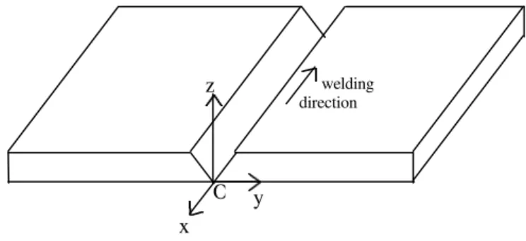
In the one-dimensional model, the heat flux is considered to occur only in the y direction, as shown in the coordinate system of Fig. 1. The following assumptions are made: the heat source moves at a sufficiently high speed (to neglect heat flux in the x direction),
Presented at COBEM 99 – 15th Brazilian Congress of Mechanical Engineering. 22-26 November 1999, São Paulo. SP. Brazil.
Paper accepted: July, 2002. Technical Editor: José Roberto de França Arruda.
and each weld pass fulfills the whole etched groove (no heat flux in the z direction).
Figure 1. Coordinate system used in the model.
The formulation of the problem to the first weld pass is made up by the one-dimensional transient heat conduction equation, and its boundary and initial conditions. It is similar to the formulation of the point heat source problem. In terms of θ (θ = T-To), it is:
2 2
y
t ∂
θ ∂ α = ∂ ∂θ
(1)
0 ) 0 t ( = =
θ (2)
0 ) y ( →∞ =
θ (3)
∫
∞
∞
− θ = ρc
Q
dy 1 (4)
where:
T = temperature (oC)
To = ambient temperature (oC) θ = temperature difference (oC) t = time (s)
y = coordinate (m)
Q1 = thermal energy per unit area (J/m2) α = thermal diffusivity of the material (m2/s)
ρ = density of the material(kg/m3) c = specific heat of the material (J/kgoC)
O
x
y
z
welding
R. N. S. Fassani and O. V. Trevisan
J. of the Braz. Soc. of Mech. Sci. & Eng. Copyright 2003 by ABCM July-September 2003, Vol. XXV, No. 3 / 303
The solution to this problem is known (Rosenthal, 1941), and it is expressed by:
α − πα ρ = θ t 4 y exp t 4 c Q ) t , y ( 2 1 (5)
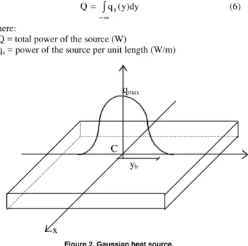
To take into account the distribution of the heat source, please refer to Fig. 2, where a source with normal or Gaussian distribution is instantaneously applied at t = 0 to the surface of a plate. The center C of the source coincides with origin O of the coordinate system xyz. The total power of the source is given by:
∫
∞
∞ −
= q (y)dy
Q s (6)
where:
Q = total power of the source (W)
qs = power of the source per unit length (W/m)
Figure 2. Gaussian heat source.
In the one-dimensional case, the Gaussian distribution of the heat source along the y direction occurs simultaneously at all points of the x direction of welding. The power qs (y) may be expressed by:
) Ay exp( q ) y (
qs = max − 2 (7)
where:
qmax = qs maximum value (W/m)
A = coefficient of arc concentration (1/m)
Coefficient A is determined considering a distance yb in Eq. (7),
which corresponds to the distance from the origin to the location where the power is reduced to five percent of its maximum value (Fig. 2). Thus,
2 b
y 3
A= (8)
When yb is large, qs(y) decreases slowly with y. Substituting Eq.
(8) in Eq. (7) and then in Eq. (6), and integrating this equation between -yb and yb limits, one obtains:
) 3 ( Erf y Q 3 q b max π = (9)
Equation (7) may then be written as:
− π = 2 b 2 b s y y 3 exp ) 3 ( Erf y Q 3 ) y ( q (10)
The diffusion process of an instantaneous Gaussian heat source applied to the surface of the material may be obtained by the source method. Let the y coordinate, along which the heat source varies, be divided in small elements dy’. The heat dQ = qs(y’)dy’ is supplied to
the element dy’ at t = 0, and may be regarded as an instantaneous point heat source. According to Eq. (5), the diffusion process to an instantaneous heat source is:
α − πα ρ = θ t 4 y exp t 4 c dQ ) t , y ( d 2 or α − πα ρ ′ ′ = θ t 4 d exp t 4 c y d ) y ( q ) t , y ( d 2 s (11)
where d is the distance between the instantaneous source and a point located on the y axis, that is,
d2 = (y-y’)2 (12)
Substituting Eqs. (10) and (12) in Eq. (11):
α ′ − − − α ρ π = θ t 4 ) y y ( exp y y 3 exp ) 3 ( Erf t 4 c y Q 3 ) t , y ( d 2 2 b 2 b (13)
By the superposition principle, the temperature change in the y point may be obtained by summing the contributions of all instantaneous concentrated sources dQ, acting along the y coordinate of the material, between -yb and yb points:
y d t y y y y Erf t c y Q t y b b y y b b ′ − − ′ ′ − =
∫
− α α ρ π θ 4 ) ( exp 3 exp ) 3 ( 4 3 ) , ( 2 2 2 (14)Solving the integral and rearranging the solution, one obtains:
+ α α + + α + α α + α − + + α α + − α + α α + α − + α π ρ = θ ) y t 12 ( t 2 y yy t 12 Erf ) y t 12 ( t 4 y y t 4 y exp ) y t 12 ( t 2 y yy t 12 Erf ) y t 12 ( t 4 y y t 4 y exp ) 3 ( Erf ) y t 12 ( c 2 Q 3 ) t , y ( 2 b 2 b b 2 b 2 b 2 2 2 b 2 b b 2 b 2 b 2 2 2 b (15)
Analytical Modeling of Multipass Welding Process with …
/ Vol. XXV, No. 3, July-September 2003
ABCM
304
In Eq. (16), it may be observed that the t variable was displaced by a value tp, which corresponds to the sum of the welding and
waiting times to the beginning of the second pass. The use of indices 1 and 2 in the qs variable is for possible and sought variations of the
heat input between passes. The same steps applied to obtain Eq. (15) are used to reach the solution for the second pass, and so on. Analogously, the general solution to n passes, in terms of T, is given by:
} } y t ) 1 i ( t [ 12 ]{ t ) 1 i ( t [ 2
y yy ] t ) 1 i ( t [ 12 Erf
]} t ) 1 i ( t [ 12 { t ) 1 i ( t [ 4
y y t
) 1 i ( t [ 4
y exp
} y t ) 1 i ( t [ 12 ]{ t ) 1 i ( t [ 2
y yy ] t ) 1 i ( t [ 12 Erf
]} t ) 1 i ( t [ 12 { t ) 1 i ( t [ 4
y y t
) 1 i ( t [ 4
y {exp
* y ] t ) 1 i ( t [ 12
Q c
2 3 T ) t , y ( T
2 b p p
2 b b p
p p
2 b 2
p 2
2 b p p
2 b b p
p p
2 b 2
p 2 n
1
i 2
b p i o
+ − − α − − α
+ + − − α
− − α − − α + − − α −
+
+ − − α − − α
+ − − − α
− − α − − α + − − α −
+ − − α π ρ +
=
∑
=
(17)
Equation (17) is the solution to the temperature distribution in one-dimensional multipass welding processes, supplied by Gaussian heat sources. Far from the heat source, i.e., for distances where y is of the same magnitude as yb, Eq. (16) is similar to the solution
obtained for the point heat source. However, near the FZ and HAZ (y<<yb), the correction introduced by the distributed heat source
approach in Eq. (17) allows to better predicting the temperatures in these regions.
Model Evaluation
A comparison between concentrated and distributed heat source models was made through simulation of thermal cycles for three weld passes. Equation (17) was used to calculate the temperatures near the fusion zone, when a Gaussian distributed heat sources is applied. The multipass model with concentrated heat source is given by Eq. (16). In this case, the variable qs(y) does not have a
distribution, and it is calculated by:
δ η = =
v VI Q
qs (18)
where:
η = arc efficiency (%) V = welding voltage (V) I = welding current (A) v = welding speed (m/s)
δ = plate thickness (m)
The waiting time (time between passes) used corresponds to 60 seconds, and the welding process was simulated during a total time of 300 seconds. The ambient temperature is 25oC. The error function in Eq. (17) was evaluated using a polynomial approximation. The properties and parameters used in the simulation are described below.
Material. The evaluation of the proposed model was made considering butt welding of high strength low alloy steel (HSLA) plates, with dimensions 0.13 x 0.10 x 0.25 m (thickness x length
bead x width). Table 1 shows the physical properties used in the simulation. It is known that the physical properties of the metal change with temperature. However, this variation in the analytical models results in a non-linear equation, and it is not possible to obtain the solution in closed form. Then, the physical properties are usually taken at a specific temperature, for example, at half the melting point of the material. In this work, they were calculated at 800oC. The values refer to low carbon steels, but they can be used for HSLA steel, as suggested by Hanz et al. (1989).
Table 1. Physical properties of low carbon steels (Hanz et al,1989).
k (J/msoC) ρc (J/m3oC) α (m2/s) 31.67 7.14x10⁶ 4.44x10⁻⁶
Welding parameters. In order to fulfill the groove, in butt welding, the usual practice is to increase the heat input from one pass to the next. In the present simulation of a real case, the increase of heat input is obtained by increasing the welding current, the other parameters in Eq. (18) remaining unaltered. However, the current increase causes efficiency to decrease. Then, a different value of efficiency must be used in each pass. The choices of these values were based on the efficiency range for the Gas Metal Arc Welding (GMAW) process, which ranges from 66 to 85% (Svensson, 1994). The welding parameters used in the simulation are in Table 2. The heat input (HI) values were determined by Eq. (18), multiplied by the material thickness. The same HI values were used in the point and Gaussian heat source models. However, in the Gaussian heat source model, only ninety-five percent of HI was applied to the weld. In order to adjust such difference, the HI values in Table 2 were multiplied by 1.05 for the Gaussian model.
Table 2. Welding parameters used three weld passes.
Pass I (A) V (V) v (m/s) η (%) HI (x106
J/m) 1
2 3
186 235 301
26.4 26.2 25.4
0.005
80 75 70
0.79 0.92 1.07
Parameter yb. In order to verify the capability of the proposed model to reproduce the thermal cycles, some values were chosen for the y and yb variables. These choices took into account the heat
input used in the simulation, and also known values of yb from the
literature, obtained via experimental determination. Table 3 shows the yb values obtained by Kou and Wang (1986), Zacharia et al.
(1989), and Wu (1992), as well as the heat input (HI) used in their analyses. In the present work, the yb parameter was estimated based
on the heat input values showed in Table 3. In Eq. (8), the A coefficient was determined for the yb distance, where the power is
reduced to five percent of its maximum value. According to this equation, by increasing the heat input parameter yb also increases,
such that the area under the curve of Fig. 2 remain equal to ninety-nine percent of its qmax value. Therefore, different values of yb for
each pass were considered, since the heat input increased in the second and third passes. The yb values used in the simulation were
0.004; 0.0047 and 0.0054 m for the first, second and third pass, respectively.
Table 3. Heat input and yb values in the literature.
Author I
(A)
V (V) V (m/s)
HI (x106J/m)
yb (m)
Kou and Wang (1986) Zacharia et al. (1989)
Wu (1992)
100 175 200
11 14 20
0.0055 0.0034 0.010
0.20 0.72 0.40
R. N. S. Fassani and O. V. Trevisan
J. of the Braz. Soc. of Mech. Sci. & Eng. Copyright 2003 by ABCM July-September 2003, Vol. XXV, No. 3 / 305
Results and Discussion
To compare the point and Gaussian heat source models, thermal cycles were simulated at two different y locations, namely: y equal to 0.001 m, appropriate for a position near the fusion zone (y < yb),
and y equal to 0.003 m, a location at a distance of the same magnitude as the yb parameter.
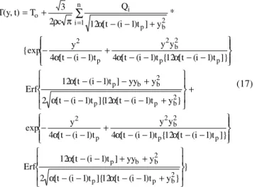
Figure 3 shows the thermal cycles obtained after the point and Gaussian heat source models, at y = 0.001 m. It can be observed that the peak temperatures in each pass are higher for the point heat source model than for the Gaussian heat source model. This occurs due to the assumption that the heat input is instantaneously applied over an infinitesimal volume cross-sectioned by the thickness-width plane at the center of the workpiece. In the Gaussian heat source model, it is assumed that the heat input is applied over the finite volume, including the y coordinate at the extent of the yb parameter.
Therefore, the peak temperatures produced by the latter model is expectedly more realistic. The previous determination of the peak temperature to be reached at a specific location is interesting, since it indicates fortuitous phase changes. The differences between the temperatures simulated by the two models are described in the Table 4. T1 refers to maximum temperature reached in the first pass; T2 in
the second pass, and so on. It is worth noticing that the correction in the proposed model affect only the peak temperature determination, and no difference is seen in the cooling rate.
Table 4. Peak temperatures reached in each weld pass.
Tpeak Point heat source Gaussian heat source
T1 2057.52 1632.28
T2 2535.16 1881.01
T3 3044.18 2115.27
0 100 200 300
t (s)
0 500 1000 1500 2000 2500 3000 3500
T
(
o
C
) point
Gaussian
Figure 3. Thermal cycles for the point and Gaussian heat source models, at y = 0.001 m.
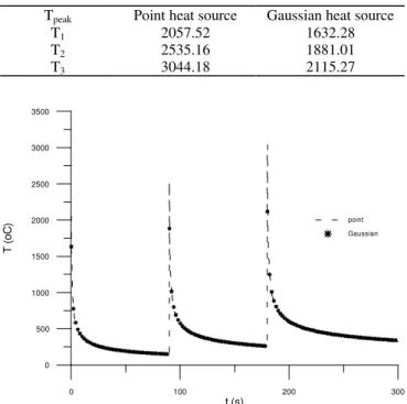
In Figure 4, the thermal cycles were simulated using y = 0.003 m. It is instrumental to show that, if y is close to yb, the Gaussian
heat source model is equivalent to the point heat source solution. The two models provide results that are practically the same. This means that the point source model at distances far from the fusion zone can correctly predict the temperature fields.
0 100 200 300
t (s)
0 500 1000 1500
T
(
o
C
)
point
Gaussian
Figure 4.- Thermal cycles for the point and Gaussian heat source models, at y = 0.003 m.
Conclusions
The main conclusions of this work are:
- the closed form solution obtained allows to estimate the thermal cycles produced by multipass welding process, near the fusion and heat affected zones;
- the distributed heat source in the proposed solution is an important correction for the known model with point source, since this factor allows to obtain temperature values more realistic near to the fusion zone;
- the analytical solution derived from the point source model can be safely used to predict temperature fields away from the fusion zone (FZ) and the heat affected zone(HAZ).
Acknowledgement
The authors want to acknowledge the financial support of FAPESP - Fundação de Amparo à Pesquisa do Estado de São Paulo - to the research work reported in the present paper.
References
Goldak, J., Bibby, M., Chakravarti, A., 1984, A new finite element model for welding heat sources, Metallurgical Transactions B, vol. 15B, pp. 299 - 305.
Hanz, Z., Orozco, J., Indacochea, J. E., Chen, C. H., 1989, Resistance spot welding : a heat transfer study, Welding Journal, vol. 68, n. 9, pp. 363s - 371s.
Kou, S., Wang, Y. H., 1986, Weld pool convection and its effect, Welding Journal, vol. 65, n. 3, pp. 63s - 70s.
Pavelic, V., Tanbakuchi, R., Uyehara, O. A., Myers, P. S., 1969, Experimental and computed temperature histories in Gas Tungsten Arc Welding of thin plates, Welding Journal, vol. 48, n. 7, pp. 295s - 305s.
Rosenthal, D., 1941, Mathematical theory of heat distribution during welding and cutting, Welding Journal, vol. 20, n. 5, pp. 220s - 234s.
Suzuki, R. N., 1996, Solução Analítica para Distribuição de Temperatura no Processo de Soldagem MIG com Múltiplos Passes, Tese Mestrado, Universidade Estadual de Campinas, Campinas, São Paulo, Brasil.
Svensson, L. E., 1994, Arc welding process, in Control of Microstructures and Properties in Steel Arc Welds, CRC Press.
Wu, C. S., 1992, Computer simulation of three-dimensional convection in traveling MIG weld pools, Engineering Computations, vol.9, pp. 529 - 537.