Reversible limit of processes of heat transfer
(Limite revers´ıvel de processos de transferˆencia de calor)J¨
urgen F. Stilck
1, Rafael Mynssem Brum
21
Instituto de F´ısica e Instituto Nacional de Ciˆencia e Tecnologia de Sistemas Complexos, Universidade Federal Fluminense, Niter´oi, RJ, Brasil
2
Instituto de F´ısica, Universidade Federal Fluminense, Niter´oi, RJ, Brasil
Recebido em 23/2/2013; Aceito em 2/3/2013; Publicado em 30/10/2013
We study a process of heat transfer between a body of heat capacityC(T) and a sequence ofN heat reser-voirs, with temperatures equally spaced between an initial temperature T0 and a final temperature TN. The body and the heat reservoirs are isolated from the rest of the universe, and the body is brought in thermal contact successively with reservoirs of increasing temperature. We determine the change of entropy of the com-posite thermodynamic system in the total process in which the temperature of the body changes fromT0 to TN. We find that for large values ofN the total change of entropy of the composite process is proportional to (TN−T0)/N, but eventually a non-monotonic behavior is found at small values ofN.
Keywords: second law of thermodynamics, entropy, reversible and irreversible processes, heat exchange.
Estudamos um processo de transferˆencia de calor entre um corpo de capacidade t´ermicaC(T) e uma sequˆencia deN reservat´orios t´ermicos cujas temperaturas s˜ao uniformemente espa¸cadas entre a temperatura inicialT0 e a temperatura finalTN. O corpo e os reservat´orios t´ermicos s˜ao isolados do resto do universo e o corpo ´e colocado em contato t´ermico sucessivamente com reservat´orios de temperatura crescente. Determinamos a varia¸c˜ao de entropia do sistema termodinˆamico composto no processo total, em que a temperatura do corpo varia deT0 a TN. Encontramos que para valores grandes de N a varia¸c˜ao total de entropia ´e proporcional a (TN−T0)/N, mas eventualmente um comportamento n˜ao monotˆonico surge em valores pequenos deN.
Palavras-chave: segunda lei da termodinˆamica, entropia, processos revers´ıveis e irrevers´ıveis, troca de calor.
1. Introduction
One of the original formulations of the second law of thermodynamics, due to Clausius, states that “no pro-cess is possible whose only result is the transfer of heat from a body of lower temperature to a body of higher temperature”. As discussed by Fermi in his book [1], since as this statement was made the concept of temper-ature was empirical, to find out which of two bodies has the higher temperature one had to put them in thermal contact and find out in which sense the heat flows, it will flow spontaneously from the body of higher temper-ature to the other. So, Clausius’s statement could be rephrased into “If heat flows spontaneously from body A to body B, no process is possible whose only result is the transfer of heat from body B to body A”. To be more precise, let us isolate the two bodies from the rest of the universe, to assure that they will not exchange heat or other forms of energy with the environment, this is implicit in the term ‘only result’. We may notice in this statement that already the idea of irreversibility is
present: if heat flows spontaneously from A to B, it will not flow spontaneously from B to A. In other words, the process of transfer of heat between two bodies which are isolated from the environment isirreversible.
The second law off thermodynamics says that not all processes which conserve energy, as required by the first law, occur in nature. In many cases (if not all), if a given process in an isolated system occurs, the inverse process does not. This idea was further formalized by the introduction of the concept ofentropy, so that pro-cesses in isolated systems which lead to a decrease of the entropy are not allowed. In particular, in the process of heat transfer mentioned above, the entropy of the com-posite isolated system increases if the heat flows from the body of higher temperature to the one of lower tem-perature, but woulddecreasein the inverse process, so that only the further is allowed. It is interesting to re-call that in his paper of 1885, Clausius summarized the two first laws of thermodynamics in just two sentences: “The energy of the universe is constant. The entropy of the universe tends to a maximum” [2]. We may notice
1
E-mail: [email protected].
that the universe is the only composite thermodynamic system which is isolated by definition.
The entropy in equilibrium thermodynamics is a state function, so that it is defined for equilibrium states of the system. When two bodies of different tempera-tures are brought into thermal contact, the composite system in general will go through a sequence of non-equilibrium states, but if we wait long enough, it will finally reach a new equilibrium state, where both bod-ies of the composite have the same temperature, and in this state the entropy is larger than it was in the initial state. If we now imagine a process which happens at a very slow rate in time when compared to the relax-ation time of the system [3], we may reach a siturelax-ation close to the one in which all intermediate states of the system are equilibrium states. In this limit the process is called quasi-static, and therefore the whole process may be represented as a path in the space of variables which define the equilibrium states of the system. In the particular case in which the entropy of the final state of the quasi-static process is equal to the entropy of the initial state, and therefore to the entropies of all intermediate states, this process will bereversible.
The process we will study in some detail here is the transfer of heat in isolated systems composed by a heat reservoir (constant temperature) and a body whose heat capacity is described by a function of the temperatureC(T). The initial temperature of the body isT0and its final temperature isTN. The change of the
temperature of the body is accomplished by putting it in thermal contact with a sequence ofN heat reservoirs whose temperatures are equally spaced betweenT0and
TN. For a finite number of reservoirs, each of the
sub-processes consists of heat transfer between two bodies at different temperatures and is therefore irreversible, leading to an increase of the entropy of the composite isolated system. In the limit N → ∞, however, each sub-process will contribute with a negligible increase of entropy and, what may not be obvious initially, the to-tal variation of entropy vanishes as well, so that this is a concrete example of a limit which leads to a reversible, quasi-static process of heat transfer.
This problem, of considerable pedagogical interest, has been studied before in the literature. For a con-stant heat capacity, such as is found for ideal gases, Calkin and Kiang [4] have shown for a cyclic process (T0→TN →T0), that the total change of entropy van-ishes as 1/N in the limit N → ∞ because, although the number of sub-processes increases, the increase of entropy in each of them is proportional to 1/N2 in this limit. A similar situation is proposed in the ex-ercise 4.4-6 in Callen’s book [3]. The same process was studied also by Thomsen and Bers [5], again for the case of constant heat capacity and discussing in detail that it is always possible, given any positive valueϵ, to choose a value ofN for which the increase of entropy is smaller thanϵ. This argument is then repeated for the inverse process, thus characterizing the process in the
limitN → ∞as reversible.
Here we generalize the problem in two ways: the heat capacity of the system is no longer constant and we develop the increase of entropy as a series in 1/N, so that we find the corrections to the leading term. We also show that some symmetries in the result which are valid in the asymptotic limit close to reversibility are not longer present for finite values of N. In particu-lar, we show that, although in the large N limit the increase of entropy decreases monotonically with N, this may not happen at lower numbers of heat reser-voirs. Also, the increase of entropy for the direct pro-cess (T0 →TN) may be different of the same quantity
for the inverse process (TN →T0). The determination of the change of entropy is given in section 2 and appli-cations to particular cases and final comments may be found in section 3.
2.
Determination of the change of
en-tropy
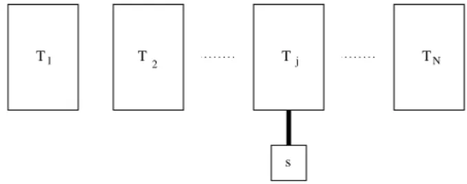
Let us define the problem in more detail. Our com-posite system consists of the body, whose heat ca-pacity is C(T) and which will undergo a temperature change ∆T =TN −T0, and a set ofN heat reservoirs, at equally spaced temperatures, so that the tempera-ture of the reservoir j (j = 1,2,3, . . . , N) is equal to
Tj =T0+j∆T /N. The body is brought into thermal contact with the heat reservoirs in order of increasing values of j until its temperature equals the one of the reservoir and therefore is increased bi ∆T /N. In the first sub-process, for example, the body starts with tem-perature T0 and ends with temperature T0+ ∆T /N. After the N’th process, the body will reach the final temperature TN. This sequence of heat transfer
pro-cesses is illustrated in Fig. 1. Actually, one could ar-gue that the time required to reach equilibrium for each sub-process of heat transfer would be infinite, and for this reason, Thomsen and Bers, in their discussion of a similar process [5], have chosen the temperature of thej’th reservoir to beT0+ (j+ 1)∆T /N, thus assur-ing that the equilibration time of the system with each reservoir is finite. Here, for simplicity, we will not use this improved version of the process.
2
T
1
T Tj TN
s
If a the body, at temperature T, receives a quan-tity of heat dQb, its temperature will change bydT =
dQb/C(T). The change of entropy of the body in the
whole sequence of heat transfer processes is
∆Sb=
∫ TN
T0
dQb
T =
∫ TN
T0
C(T)
T dT.
The change of entropy of all reservoirs in the sequence of processes will be
∆Sr(N) = N
∑
j=1
∆Sr(N, j) = N
∑
j=1 1
Tj
∫ Tj
Tj−1
dQr=
− N
∑
j=1 1
Tj
∫ Tj
Tj−1
C(T)dT, (1)
where in the last passage, we recall that in each sub-process, the body and the reservoir are isolated, so that the heat received by the reservoir is given by
dQr = −dQb = −C(T)dT. We thus may write the
total change of entropy as
∆S(N) = ∆Sb(N) + ∆Sr(N) =
∫ TN
T0
C(T)
T dT−
N
∑
j=1 1
Tj
∫ Tj
Tj−1
C(T)dT. (2)
If it is possible to perform both integrations, this ex-pression above becomes
∆S(N) =Sb(TN)−Sb(T0)− N
∑
j=1 1
Tj
[U(Tj)−U(Tj−1)],
(3) where Sb(T) = ∫C(T)/T dT and U(T) = ∫C(T)dT.
It is convenient to rewrite the expression for the change of entropy as
∆S(N) =
N
∑
j=1 ∫ Tj
Tj−1
κj(T, N)ϕ(T)dT, (4)
where κj(T, N) = 1−T /Tj and ϕ(T) = C(T)/T. It
is now easy to see that, since stability implies that
ϕ(T)≥0, we must have ∆S ≥0, as required by the sec-ond law of thermodynamics. Let us show this in some detail. Suppose thatTN > T0, so that the temperature of the body increases in the process. It is then clear that κj(T, N)≥0 and as a consequence the entropy of
the composite system increases. The same happens in the inverse process, where the temperature of the body decreases from TN to T0. In this case the change if entropy is
∆S′
(N) =− N
∑
j=1 ∫ Tj
Tj−1
κj−1(T, N)ϕ(T)dT, (5)
and since now κj−1(T, N) ≤ 0 in the range of inte-gration, again the entropy increases. It may be worth
noticing that the difference of the entropy increases be-tween the processes with raising and lowering of the temperature of the bodyδS(N) = ∆S′
(N)−∆S(N) is
δS(N) =
N
∑
j=1 ∫ Tj
Tj−1
[( 1
Tj−1 + 1
Tj
)
T−2 ]
ϕ(T)dT,
(6) and the sign of this expression is not defined in general. Another general property of the entropy increase is its dependence of the number of reservoirs N. As we will see below, it vanishes in the limit N → ∞ of a quasi-static process. The question we will address is if the change of the entropy decreases monotonically with
N. For convenience, we will define the function
κ(T, N) =
N
∑
j=1
Θ(T−Tj−1)Θ(Tj−T)κj(T, N), (7)
where Θ(T) is the step function. The functionκ(T, N) is defined in the whole temperature range [T0, TN] and
has a sawtooth pattern, withN maxima of decreasing values. The expression for the entropy increase Eq. (4) may then be cast into the following form
∆S(N) = ∫ TN
T0
κ(T, N)ϕ(T)dT. (8)
The difference of entropy increases for two values ofN, (N2> N1) is
∆S(N1)−∆S(N2) = ∫ TN
T0
[κ(T, N1)−κ(T, N2)]ϕ(T)dT. (9) It is straightforward to see that ifN2 is a multiple of
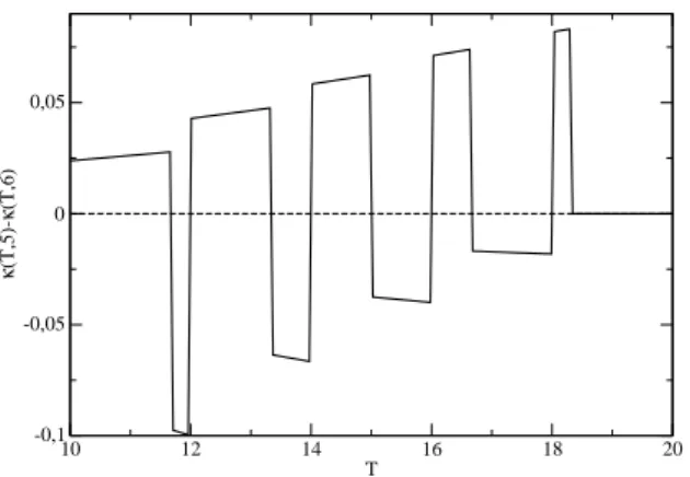
N1 the difference of κ functions is non-negative, and therefore ∆S(N1)−∆S(nN1) ≥ 0 for any integer n. For example, we have ∆S(1)>∆S(2). This, however, is no longer true in general if the ratio N2/N1 is not an integer. As an example, in Fig. 2 we show the dif-ference of κ functions for N1 = 5 and N2 = 6, and we notice that this difference assumes negative values in part of the temperature domain. We thus reach the conclusion that, depending on the function ϕ(T), the entropy increase for N2 heat reservoirs may be larger than the one forN1 reservoirs, if 1< N2/N1<2.
We now proceed obtaining the general asymptotic behavior of ∆S(N) for N ≫ 1. Expanding the last integral in the expression for the increase of entropy, Eq. (2), which corresponds to the amount of heat Qj
exchanged by the body with reservoir j, in a Taylor series around the temperatureTj, we get
Qj=−
∞ ∑
i=1 (−1)i
i
(∆T
N
)i
C(i−1)(T
10 12 14 16 18 20 T
-0,1 -0,05 0 0,05
κ
(T,5)-κ
(T,6)
Figure 2 - The functionκ(T,5)−κ(T,6) for initial temperature T0= 10 and final temperatureTN= 20.
where a superscript between parenthesis means a derivative of the corresponding function of the order of the superscript. We may now write the total change of entropy as
∆S(N) = ∫ TN
T0
C(T)
T dT+
∞ ∑
i=1 (−1)i
i
( ∆T
N
)i N ∑
j=1
C(i−1)(T j)
Tj
. (11)
We now proceed transforming the sum over the reservoirs into an integral, using Euler-MacLaurin’s ex-pansion [6]
n
∑
i=m
f(i) = ∫ n
m
f(x)dx+1
2[f(n) +f(m)] +
kmax
∑
k=1
B2k
(2k)! [
f(2k−1)(n)−f(2k−1)(m)]+R
kmax, (12)
where B2k are the Bernoulli numbers (B2 = 1/6,
B4=−1/30,B6= 1/42,B8=−1/30,. . .. See Ref. [7] for a list of the numbers). The series in the right hand side is divergent in many cases, since the Bernoulli num-bers increase very fast for larger values ofk. There are procedures to evaluate the rest Rkmax [6] and we will
discuss this issue in the appendix. The sum we will convert into an integral is
Gi= N
∑
j=1
C(i−1)(T j)
Tj
=
N
∑
j=0
C(i−1)(T j)
Tj
−C
(i−1)(T 0)
T0
,
(13) and applying the expansion (12) we find
Gi =
N
∆T
∫ TN
T0
C(T)(i−1)
T dT+
1 2
[
C(i−1)(T N)
TN
−C
(i−1)(T 0)
T0 ]
+
kmax
∑
k=1
B2k
(2k)! (
∆T N
)2k−1 ×
[(
C(i−1)(T N)
TN
)(2k−1)
−
(
C(i−1)(T 0)
T0
)(2k−1)]
+Rkmax. (14)
Now we may substitute this last expression into Eq. (11) and collect the terms in the change of entropy of the body in the sequence of processes in powers of 1/N. We notice, as expected, than the term of order 0 cancels, so that, in the limit N → ∞the whole pro-cess becomes reversible. In the appendix, we proceed calculating all coefficientsσi of the expansion
∆S(N) =
imax
∑
i=1
σi
(1
N
)i
, (15)
but here we we will limit ourselves to the leading term, which is
σ1=
TN −T0
2 ×
[ ∫TN
T0
C(1)(T)
T dT−
(
C(TN)
TN
+C(T0)
T0 )]
. (16)
Integrating by parts, we finally obtain the leading term of the expansion
∆S(N)≈ TN−T0
2N
∫ TN
T0
C(T)
T2 dT, (17)
valid in the limitN ≫1.
Since C(T) ≥ 0, we notice that the leading term vanishes only in the trivial case where C(T) = 0 in the whole range of temperatures and there is no heat transfer, so that the asymptotic behavior as 1/N in the increase of entropy, as was found in the particular case of an ideal gas [4], is universal. We also remark that in the asymptotic regime the entropy increase is invariant if the temperatures are interchanged and also monoton-ically decreasing withN, properties which are not true in general for small values of the number of reservoirs.
3.
Discussions and conclusion
C(T) =C0. Applying Eq. (2) to this particular case, the increase of the entropy will be
∆S(N)
C0
= lnf−f−1
N
N
∑
j=1
1
1 +Nj(f −1), (18)
where f =TN/T0. The leading term in this case is ∆S(N)
C0
≈ 1
2N
(√
f−√1/f)2. (19)
In Fig. 3 we show some curves of the entropy increase as a function of 1/N, for different values of the ratio of temperaturesf, as well as the dashed straight lines which represent the asymptotic behavior. Notice that, as expected, the same asymptotic behavior is found for
f = 2 and f = 1/2. If we consider two processes, one with ratio f1 > 1 and the other with f2 = 1/f1 < 1, that is, related by interchange of the temperatures, both will have the same asymptotic behavior, as may be seen in the particular cases depicted in the figure. Also, the increase of entropy in the second process, where the body is cooled, is always larger than the one in the first process. Another way to state the same property is that, as can be seen in the curves, the increase of en-tropy is a concave function of 1/N for processes where the body is heated and it is a convex function when the temperature of the body decreases. In the asymptotic regime these properties may be obtained the next term of the Euler-MacLaurin expansion, as will be discussed in the appendix. Also, the increase of entropy for this particular case is a monotonically decreasing function ofN.
0 0,2 0,4 0,6 0,8 1
1/N 0
0,5 1 1,5 2 2,5 3
∆
S/C
0
Figure 3 - Increase of entropy for a system with constant heat capacity C0 (ideal gas) as a function of the inverse number of reservoirs 1/N. The four curves, in the upward order, correspond to ratios of temperaturesf =TN/T0 = 2, 1/2, 5 and 1/5. The dashed straight lines are the asymptotic behavior for small 1/N.
In most cases the variation of entropy decreases monotonically withN, a property which seems also in-tuitive, since by decreasing the temperature steps in a certain sense the composite process gets closer to a re-versible process. For the ideal gas this is always the case. We have seen above, however, that this may not be generally true. If we look at the Eq. (9) for the
difference of entropy increases for different values of
N, a non-monotonic result is possible if the function
ϕ(T) has one or more peaks at the temperatures where
κ(T, N1)−κ(T, N2) is negative. One system which could possibly show a non-monotonic behavior is a two-state system [3], since its heat capacity displays a peak, sometimes called “Schottky hump”. However, we found that this is not the case, the reason is that the peak is too wide to produce a non-monotonic behavior.
We turn our attention to a situation where the width of the peak in the heat capacity may be changed by ad-justing a parameter. The simple expression we will use for the heat capacity is
C(T) =C[τ(2−τ)]m, (20)
where τ =T /Tc, so that Tc is the temperature where
the maximum of the heat capacity is located, andCis a constant with the dimension of entropy. Although this heat capacity does not correspond to a particular phys-ical system, it is convenient for analytic calculations and consistent with the third law of thermodynamics. Of course, at least for odd values of the parameterm, it is valid only ifτ is in the range [0,2], so we will re-strict ourselves to this range of temperatures. As the parameter m grows, the peak in C(T) narrows, and our main interest in this system is that, for sufficiently large values ofm, non-monotonic behavior is found in ∆S(N).
In Fig. 4 we show, in the same graph, the function
κ(τ,2)−κ(τ,3) and the function ϕ(τ) = C(τ)/(Cτ), given by Eq. (20) withm= 16. As is apparent in the graph, with the choices of initial (τ0= 0.286) and final (τN = 2.0) temperatures we made, the maximum of the
peak inC(T) is close to the center of the negative peak inκ(τ,2)−κ(τ,3), so that the difference ∆S(2)−∆S(3) is minimized, since this difference is given by Eq. (9). In Table 1 we list the results for [∆S(3)−∆S(2)]/C
for different values ofm, with the choices above for τ0 andτN, and it is clear that a non-monotonic behavior is
found form≥16. Finally, we found some evidence that a local maximum in the entropy could also be found at
N = 4, but if this actually happens for this particular form of heat capacity, it will be at rather large values of
m, which lead to numerical problems. We remark that, in order to reduce numerical errors, in all examples we discuss the integrations involved in the calculation of the entropy increase Eq. (2) are performed analytically, as is done in Eq. (3).
Table 1 - [∆S(3)−∆S(2)]/C for different values of the param-etermfor a system with heat capacity given by Eq. (20). The temperature range of the process isτ0= 0.286,τN= 2.0
0,5 1 1,5 2 τ
0 0,5 1
κ(τ,2)−κ(τ,3); φ(τ)
Figure 4 -κ(τ,2)−κ(τ,3) (dashed line) and the functionφ(τ) = C(τ)/(Cτ) = [τ(2−τ)]16
/τ. The initial temperature isτ0 = 0.286 and the final temperature isτN= 2.0.
As discussed before, we expect, qualitatively, the non-monotonic behavior to be enhanced if the peak in the heat capacity is more pronounced. This leads us, in this final example, to a system which undergoes a con-tinuous phase transition, since in this case a singularity at the critical temperatureTc is found in the heat
ca-pacity, of the formC(T)≈ |1−T /Tc|−α, described by
the critical exponentα[8]. To the singular behavior of the heat capacity, usually regular contributions should be added, so that we will use the simple expression
C(T) =Cτ|1−τ|−α, (21)
where we define the reduced dimensionless temperature
τ =T /Tc and which is compatible with the third law
of thermodynamics. It should be mentioned that since the exchange of heat when the temperature of the body crosses the critical temperature has to be finite, we should restrict the critical exponentαto values smaller than 1. It is easy to perform the necessary integrations in this case, so that the entropy increase will be given by Eq. (3) with
Sb(τ)
C =
−(1−τ)1−α
1−α , τ <1, (τ−1)1−α
1−α τ≥1,
(22)
and
U(τ)
CTc
=
− (1−τ)1−α
(1−α)(2−α)[1 + (1−α)τ], τ <1 (τ−1)1−α
(1−α)(2−α)[1 + (1−α)τ], τ≥1. (23)
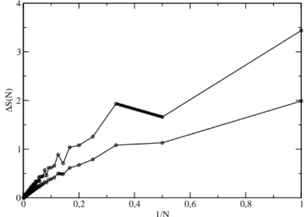
We would expect that the non-monotonic behavior of the entropy should be enhanced as the value of the critical exponentαincreases. This is actually true, but at variance with what is seen in the preceding example of a peak in the heat capacity, the local maxima of the entropy increase, for lower values ofα, appear at larger values of N. In Fig. 5 we see results of the increase of entropy for two values of the exponent,α= 0.7 and
α= 0.5. It is apparent that, forα= 0.7 we already have
an increase of the change of entropy between N1 = 2 and N2 = 3, the segment with a thicker line in the curve. Many other pairs of successive results with the same property are found for larger values of N. For
α= 0.5, the first pair where the change of entropy in-creases is seen atN1= 7,N2= 8.
0 0,2 0,4 0,6 0,8 1
1/N 0
1 2 3 4
∆
S(N)
Figure 5 - Values of ∆S(N) as function of 1/Nfor a body with a continuous phase transition (Eq. (21)). The upper curve is for α= 0.7 and the lower one forα= 0.5. The pairs of data at the end of the thick lines are the first ones, in the order of increasing values ofN, where a increase of ∆S(N) is found. These results are forτ0= 0.2 andτN= 2.2.
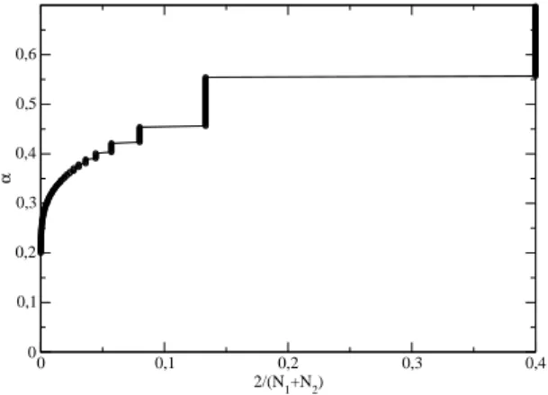
For a given a value of the critical exponent α, we may findN1, the lowest value ofNsuch that ∆S(N2)> ∆S(N1), whereN2 =N1+ 1. In Fig. 6, the exponent
αis plotted as a function of 2/(N1+N2), and we no-tice that, at least for large values of α, that the func-tion shows steps. The results shown are calculated for
τ0= 0.2 andτN = 2.2. Thus, for example, ifα >0.555,
we notice that the first increase of ∆S(N) is seen be-tween N1 = 2 and N2 = 3, while if αis in the range [0.555,0.454] this increase is seen at N1 = 7, N2 = 8, ifαis further decreased the increase shifts toN1= 12,
N2 = 13, and so on. This pattern, although qualita-tively remaining the same, changes quantitaqualita-tively for a different temperature range. We notice an interest-ing behavior for small values of α, which leads to the question if, for any positiveα an increase if ∆S(N) is found for a finite value ofN. Due to round-off errors, we could not address this question numerically. How-ever, since the coefficients σi in the Euler-MacLaurin
expansion Eq. (15) diverge in this case for i > 1 and any positive α, the answer to this question should be positive. We discuss this point somewhat more in the appendix.
Finally, we notice that, in opposition to what was found in the first two examples we studied, when the body undergoes a continuous phase transition it is pos-sible that ∆S(N) > ∆S′
(N), that is, the increase of entropy in the heating process is larger than the one in the cooling process, a possibility which was antici-pated in the discussion after Eq. (6). In Fig. 7 we present results for the difference in entropy increases ∆S′
func-tions of 1/N. The temperature interval is τ0 = 0.2,
τN = 2.2 Although in most cases this difference is
pos-itive, forα= 0.7 already forn= 13 we get a negative result, and a set of values ofN above this one have the same property. For α = 0.5 the effect is smaller, and the first occurrence of a negative result is forN = 88. Again it would be interesting to study more details of these results at large values ofN, but round-off errors prevent this to be done numerically.
0 0,1 0,2 0,3 0,4
2/(N
1+N2)
0 0,1 0,2 0,3 0,4 0,5 0,6
α
Figure 6 - Values of the critical exponentα for which the first increase of ∆S(N) if found betweenN1andN2=N1+1, as func-tion of 2/(N1+N2). The data are forτ0= 0.2 andτN= 2.2.
0 0,02 0,04 0,06 0,08 0,1
1/N 0
0,1 0,2 0,3
∆
S
’
(N)-∆
S(N)
Figure 7 - Difference in the increases of entropy in the cooling and the heating processes ∆S′(N)−∆S(N), for τ0 = 0.2 and
τN = 2.2. The curve with larger oscillations is forα= 0.7 and the other one forα= 0.5.
A final remark on this example is that, if τ ≪ 1,
C(τ)≈Cτ, so that it will show a behavior similar to a gas of non-interacting fermions at low temperature. In this case, if the initial temperatureτ0approaches 0, the coefficientσ1diverges as a logarithm. In other words, in a heating process starting atτ0= 0, the tangent to the curve ∆S×1/N at the origin is vertical. This curve is concave, sinceσ2is negative. The even more unphysical cooling process with vanishing final temperature shows a very uncommon behavior: ∆S(N) diverges for any finite N and vanishes asN → ∞.
In conclusion, we notice that in general the process of heat transfer between a body and a sequence of heat reservoirs, is a very rich physical situation for under-standing of the second law of thermodynamics and the
concept of a reversible process. In particular, if the body undergoes a continuous phase transition in the composite process, some curious phenomena appear , which at first seem to defy common sense, but of course none of them violates thermodynamics.
Appendix: Euler-MacLaurin expansion
Here we will develop the terms of the Euler-MacLaurin expansion in some detail. If we substitute Eq. (14) into Eq. (11) and collect the terms in the change of entropy of the body in the sequence of processes in powers of ∆T /N. We notice, as expected, than the term of order 0 cancels, so that, in the limitN → ∞the whole pro-cess becomes reversible. The coefficients we obtain for the change of entropy Eq. (15) are
σi= (−1)i(TN−T0)i {
−1 (i+ 1)
∫ TN
T0
C(i)(T)
T dT+
+1 2i
(C(i−1)(T N)
TN
−C
(i−1)(T 0)
T0 )
+
[i/2] ∑
k=1
(−1)2k−1B 2k
(i+ 1−2k)!(2k)!× [(
C(i−2k)(T N)
TN
)(2k−1)
−
(
C(i−2k)(T 0)
T0
)(2k−1)]}
, i= 1,2,3, . . . (24)
The two first coefficients of this series, after integrating by parts, are:, are
σ1=
TN −T0 2
∫ TN
T0
C(T)
T2 dT, (25)
and
σ2 = −
(TN −T0)2 12
[ 4
∫ TN
T0
C(T)
T3 dT+
C(TN)
T2 N
−C(T0)
T2 0
]
. (26)
In the particular case of an ideal gas, whereC(T) =
C0, the coefficients are
σ1 = −C0TN −T0 2
( 1
TN
− 1
T0 )
, (27)
σ2k = C0B2k(TN −T0) 2k
2k
( 1
T2k N
− 1
T2k 0
)
,(28)
where the last expression is valid fork= 1,2,3,. . . . We notice that, with the exception of the dominant term, only terms with even powers of 1/N appear in the ex-pansion for this particular case. For the heating process
TN > T0,σ2<0, so that the ∆S is a concave function of 1/N in the limit N → ∞. For the cooling process
TN < T0, the function is convex. These properties can be verified in the numerical results presented in Fig. 3. Very often the expansion in the Euler-MacLaurin summation (12) does not converge. We find that even forN = 1 the truncated asymptotic values are close to the exact ones at rather low orders. However, truncat-ing at higher orders does not necessarily lead to results closer to the exact ones. For example, for N = 1 the result closest to the exact one is found truncating the series at kmax = 6. We notice that higher orders of
truncation lead to wrong results, as may be seen in Fig. 8, where the increase of entropy calculated using the expansion Eq. (15), for N = 1 and TN/T0 = 2, is shown for several orders of truncation. The results oscillate around the exact value at successive orders. The best result is obtained for kmax = 6 and if we
truncate the expansion at larger orders we observe that they start deviating from the exact value.
2 4 6 8 10 12 14
kmax 0,1
0,15 0,2 0,25
∆
Sk
max
/C
0
Figure 8 - Increase of entropy for a system with constant heat capacityC0 as a function the order of truncation of the asymp-totic expansionimax. The ratio of temperaturesTN/T0is equal to 2 and the number of reservoirs is N = 1. The exact value corresponds to the dashed line.
In the Table 2, we present more results of such cal-culations. We notice that quite accurate estimates of the entropy change may be obtained if the series is trun-cated at the most favorable order. The question of de-termining the order which minimizes the restR in the Euler-MacLaurin expansion Eq. (12) is rather technical and we refer to the specialized literature for details, but in general it may be assured that, if f(x) in Eq. (12)
has always the same sign and if the function and all its derivatives tend monotonically to 0 as x→ ∞, which are valid for f(N) = ∆S(N), then the rest Rkmax is
of the same order and has the same sign of the first neglected term [6].
Table 2 - Body with constant heat capacity (C(T) =C0). Values of the relative difference between the increase of entropy calcu-lated directly (∆S) and the one which follows truncating the series Eq. (15) (∆Skmax). Several values forTN/T0 andN are considered, and the optimal order of truncationimaxis given.
TN/T0 N kmax |∆S−∆Skmax|/∆S ∆S 1/3 1 2 6.8311×10⁻²
0.9014 1/3 2 6 4.3650×10⁻³
0.4014 1/3 3 8 2.5634×10⁻⁴
0.2538 1/3 4 12 1.2824×10⁻⁵
0.1847 1/3 5 16 6.4910×10⁻⁷
0.1450 1/3 6 18 3.0760×10⁻⁸
0.1192 1/2 1 6 5.6735×10⁻³
0.3069 1/2 2 12 1.6897×10⁻⁵
0.1402 1/2 3 18 4.0671×10⁻⁸
0.0765
2 1 6 9.0135×10⁻³
0.1931 2 2 12 2.1570×10⁻⁵
0.1098 2 3 18 4.7960×10⁻⁸
0.0765
3 1 2 1.4255×10⁻¹
0.4319
3 2 6 6.6046×10⁻³
0.2653 3 3 10 3.4783×10⁻⁴
0.1907 3 4 12 1.5940×10⁻⁵
0.1486 3 5 16 7.7345×10⁻⁷
0.1217 3 6 18 3.5619×10⁻⁸
0.1030
Finally, it is clear from Eq. (24) for the expansion coefficients, that for the case of a singular heat capacity at a critical temperatureTc (C(T) =Cτ(1−τ)α, with
τ = T /Tc), all but the first coefficients diverge if the
temperature interval includes the critical temperature. This fact may account for the rather peculiar behavior found numerically in the largeN limit.
References
[1] E. Fermi,Thermodynamics, (Dover, New York, 1956). [2] R. Clausius, Annalen der Physik und Chemie,125, 353 (1865), a translation may be found in William Francis Magie,A Source Book in Physics, (McGraw-Hill, New York, 1935).
[3] H.B. Callen, Thermodynamics and an Introduction to Thermostatistics, (John Wiley & Sons, New York, 1985).
[4] M.G. Calkin and D. Kiang, Am. J. Phys.51, 78 (1983) [5] J.S. Thomsen and H.C. Bers, Am. J. Phys. 64, 580
(1996).
[6] K. Knopp, Theorie und Anwendung der unendlichen Reihen, (Springer Verlag, Berlin, 1964).
[7] The denominators and numerators of several Bernoulli numbers may be found in the addresses http://
oeis.org/A027642andhttp://oeis.org/A000367.
re-spectively. These data are provided by the On Line Encyclopedia of Integer Sequences (http://oeis.org/ wiki/Welcome).