Thermal Physics Mathematical Modeling of Cycle Cylindrical Grinding with Radial Feed

(1)

Abstract — This article includes mathematical describing and solving task of thermal conductivity for bidimentional model of grinding thermophysics in effective processing cycle. Model takes into account processed material thermo physical parameters and following process factors: duration and intensity of acting heat source at each working piece turn, heat dissipation to process fluid, as well, as tolerance, grinded out at each working piece turn, allowing organizing effective grinding cycle.

Index Terms — Grinding, grinding cycle, grinding thermophysics

I. INTRODUCTION

RINDING is one of the main processing methods, assuring surface accuracy and quality. Grinding on grinding machines is performed according to special cycle, allowing detail manufacturing adaptation to different technological conditions. Grinding cycle includes four main stages: grinding wheel approaching, cutting-in, eliminating main allowance, and dead-stop grinding. As of now there are three main methods of grinding cycles designing: regulatory, production, and design

Regulatory cycle is based on recommendations, presented in general mechanical engineering regulations on cutting regimes [1-4]. Usually regulatory cycle consists of two steps, when main machining is performed under constant radial feed on the stage of grinding out main allowance, and with decreasing feed speed on the dead-stopping stage.

Production cycle is formed on the basis of grinding several trial work pieces [5-8] with gradual increasing of metal grinding out intensity up to determined setting level. This approach allows designing multistep cycle, where main allowance grinding out stage consists of steps, each of them having its own feed. Depending on setting, feed will vary in time.

Design machining cycle is generated on the basis of cycle parameters, obtained by calculating using empirical and semiempirical dependences [9]. Design cycles, based on data, received when modeling machining processes [10-14], recently became more actual. This method also allows

Manuscript received June 09, 2015. This work was supported in part by the President Russian Federation under Grant -873.2014.8.

A.A. D`yakonov is with department of technology of engineering in South-Ural State University, Chelyabinsk city, Russian Federation (e-mail: sigma-80@mail.ru).

I.V. Shmidt is with department of technology of engineering in South-Ural State University, Chelyabinsk city, Russian Federation (e-mail: shimdt174@mail.ru).

forming multistep cycle implementing only calculations [15, 16].

Later two methods of grinding cycles designing allow assuring quality surface under maximum possible productivity of grinding process.

Different scientists took part in working out typical grinding cycles, used in industry. Maximum feed speed value for each cycle step is taken based on process limits, such as machining accuracy, surface roughness, heat defects appearing, etc.

Grinding cycle reflects machining modes change with time sequence. Cycle control is performed by changing grinding wheel feed speed. Feed speed shifting is performed in steps, depending on remaining part of allowance and acts as a constant for each cycle step.

It should be noted that possibilities of modern progressive equipment allow programming stepless feed changing during whole machining cycle. This allows forming more complex abrasive machining cycles, taking into account physical features of the process itself.

Present theoretical investigations on designing grinding cycles allow determining physical regularities on the stages of cutting-in and dead-stopping, but they don't allow evaluating feed speeds values and their distributing over cycle steps. So, designing abrasive machining cycles on the basis of modeling, allowing taking into account physical nature of the grinding process, is a very actual task.

This article deals with one of the main restricting criteria for designing grinding cycle – limit burn-free temperature. In order to determine it we have mixed boundary problem of the third and fourth type for thermal conductivity equation in polar coordinates. Problem numerical solution is implemented in the form of the software module. Performed calculations have demonstrated that most effective way to design the cycle for maximum burns-free temperature is to recalculate feed at each following detail rotation for the whole processing cycle.

II. PROBLEM DESCRIPTION

In order to solve task of modeling temperature for grinding cycle, it is necessary to determine depth of the working piece surface layer, for which limit temperature is considered.

When taking into account temperature in cutting area on machined surface at each working piece turn as limiting temperature, than burn-free limitation is assured by constant feed over whole grinding cycle, i.e. performing single-step machining cycle. Such approach is implemented in guides on cutting modes [1-4]. This leads to decreasing productivity by constant feed over whole machining cycle.

When calculating initial feed for assuring burn-free final

Thermal Physics Mathematical Modeling

of Cycle Cylindrical Grinding with Radial Feed

Aleksandr A. D`yakonov,

Member, IAENG,

Irina V. Shmidt

G

Proceedings of the World Congress on Engineering and Computer Science 2015 Vol II WCECS 2015, October 21-23, 2015, San Francisco, USA

ISBN: 978-988-14047-2-5

ISSN: 2078-0958 (Print); ISSN: 2078-0966 (Online)

(2)

surface of the completed detail, taking into account total cut off allowance, it is necessary to take into account, that when cutting off the allowance, temperature front will spread into the working piece for the distance, equal to allowance, cut off during one turn of the working piece. This leads to forming defective layer with depth, similar to total allowance value.

Taking into account noted disadvantages, we suggest following calculating scheme – limit temperature calculating is performed for final product surface, taking into account allowance, cut off during each turn of the working piece (Fig. 1).

Taking into account feed Vsrad, heat quantity, emitted over machines surface on the first working piece rotation, is equal to Q’1, taking into account following limitation - temperature

on border between cut off allowance and final detail should not exceed limit value (Fig. 1). For working piece second and further rotations it is necessary to recalculate radial feed speed Vsrad values, taking into account decreasing left total allowance. Above mentioned limitation should also be followed. This makes it necessary to find law of radial feed speed Vsrad dependency of time, or of detail rotation.

III. CALCULATING SCHEME AND SOLVING HEAT CONDUCTIVITY TASK

Let's discuss wheel of radius R, heat capacity c per unit of volume [J/(mm³·K)]; heat conductivity q [J/(mm·s·K)]. Wheel represents a cylinder of single-unit height with heat insulated butt ends.

During processing, tolerance, equal to doubled cut depth, is cut off from the work piece surface at each work piece turn, so at each moment of time, actual wheel size is equal to

R + R’, where R’ – cut depth.

Heat source with power Q’ [J/mm2·s·K] acts on the wheel, when passing point on the wheel surface in cutting area (contact arc) with angular speed ’ [degree/s]. Heat dissipates from the processed surface: out of the heat source acting area with coefficient ’ [J/m2·s·K], inside the wheel – with coefficient ’ [J/mm3·s·K].

This allows two-dimensional description of thermo physics task with calculating scheme, presented on Fig. 2.

Heat conductivity equation for this model converts into following:

(

w T

)

w

r r w r r r w t w

− − ∂ ∂ ⋅ + ∂ ∂ ∂

∂ ⋅ = ∂ ∂ − ∂ ∂

ν ϕ ϕ

ω ₂

2

1 1

, (1)

where w=w(r’, ) – temperature [deg.];

R r

r= '; r’ – distance from wheel center [mm]; – time [s];

₂

R a t= τ ;

c q

= [mm²/s];

– angle in fixed coordinates;

q

R2

' ν

ν= ;

T – ambient temperature [degrees].

Initial conditions: temperature is considered equal to ambient temperature:

(

r

)

T

w ,ϕ,0 = , (2) where r – radial vector (r 1);

– vectorial angle. Edge conditions:

(

)

₍

₎

T w Q r

t R w

− − = ∂

∆ + ∂

µ ϕ,

, 1

, (3) where

R R R=∆ '

∆ ;

q

R Q

Q= ' ;

q

R ' µ µ= .

So, bi-directional model demonstrates the problem in the form of the heat conductivity equation and complex of edge conditions of second and third type, i.e. combined boundary problem for the equation (1).

After introducing new variable s=r2 het conductivity equation transforms into:

(

w T

)

w s s w s s w t w

− − ∂ ∂ ⋅ + ∂ ∂ ∂

∂ = ∂ ∂ − ∂ ∂

ν ϕ ϕ

ω ₂

2 1

4 , (4)

where

a R2

'

ω

= .

Now S=(1+ R)² –1. Than initial condition will transfer to:

(

r

)

T

w ,ϕ,0 = , (5) and edge condition:

(

)

₍

₎

T w Q s

t S w

− − = ∂

∆ + ∂

µ ϕ,

, 1

. (6) We divide processed circumference into m equal parts and tolerance, cut off from the work piece per one processing cycle, - into n parts; we'll discuss nodes (si, j):

si = i h, ( i = 0, 1, ..., n-1), (7) j = j , (j = 0, 1, ..., m-1), (8) where

1 2

2 − =

n

h ;

m

π

ϕ=2

∆ ;

Fig. 1. Allowance cutting off for multipass machining (Vsrad – radial feed speed [mm/min]; Vw – grinding wheel speed [m/s];

nw – working piece rotation speed [min-1]; D – working piece diameter [mm];

Lc – contact arc length [mm]; A – machining allowance [mm];

R’1, R’2, R’i – cut depth for first second, i rotation of the working piece;

Q’1, Q’2, Q’i – heat source intensity for first, second,

i working piece rotation [W/m])

Fig. 2. Calculating scheme

ISBN: 978-988-14047-2-5

(3)

as 2 2 4 4 4 s w s s w s w s s ∂ ∂ + ∂ ∂ = ∂ ∂ ∂ ∂ (9) then, defining current temperature value w(si, j, t) (t0 t t0 + t) through wij and value w(si, j, t0) through uij, we'll have:

(

∆ϕ

)

+ν + = ₂ 2 2 8 i i i s h s

q (10)

( ) , 2 4 2 , 1 , 1 , 1 , 1 2 , 1 , 1 T s u u h u u h u u s f i j i j i j i j i j i j i i ij ν ϕ + ∆ + + − + + = + − + − + − (11) than for temperature value wij, (i > 0) we'll have equation

with partial derivatives of the first order: . ij ij i ij ij f w q w t w = + ∂ ∂ − ∂ ∂ ϕ

ω (12)

For temperature value in the wheel center w00 we integrate

equation (4) per circumference with radius h/2 and take into account periodicity per and antisymmetry derivate per s in zero, resulting transferring equation in:

= + ⋅ = + ∂ ∂ m j j T m h u w q t w 0 1 00 0

00 ₄ _ν _{, (13)}

where = +ν h q0 4 .

With t= t for equation (4) we obtain following answer:

(

1

)

. 4 0 0 0 0 1 00 00 t q m j j t q e q T m h u e u

w − ∆ = − ∆

− ⋅ + ⋅ + = ν (14) Time pitch t is chosen in order to fulfill condition:

. 2

m

t π

ω ϕ= ⋅∆ =

∆ (15)

Implementing piecewise-linear interpolation per angle, and supposing that at each range [ j, j+1] for each constant s

all functions are linear per variable and uninterruptable in edge points, we receive solution of equation (12) for t= t:

(

) (

1

)

.

1 1 2 1 1 ∆ − ⋅ ⋅ − + ⋅ − + ⋅ = − ∆ − ∆ + + ∆ − + ϕ

ω ij ij

i t q t q ij ij i t q ij ij f f q e e f f q e u

w i i i (16)

At wheel border radius changes as tolerance is cut off with speed of

a R v

v= ' , where v’ – speed of tolerance cutting

off per one turn of the work piece [mm/s]. This leads to changing processed surface border configuration. Beside this, tolerance cutting off within grinding cycle is performed per spiral from one turn to another This feature will be taken into account in numerical scheme.

In particular, when cutting off tolerance, layer thickness (ring with number n-1) per one work piece turn will change along the border, meaning, will depend from j (angle number). Than in this layer and in dummy layer with number

n current layer thickness will be equal to h+2hj, where hj – half of the tolerance, cut off per one working piece turn.

Than for i=n–2 we have:

(

)

(

)(

)

(

)

(

)(

)

( )

. 2 4 2 8 2 1 , 1 , , 1 2 , 1 2 , 1 , 1 T s u u h h h h h u h h u h h h h h h u h h hu s f i j i j i i i j i i j i i i j i i j i i ij ν ϕ + ∆ + + + + + + − + + + + + = − + − + − + (17)

For i=n-1 we have:

(

)

(

)

(

)(

)

(

)

(

)

(

)(

2

)(

2 3

)

( )

.

2 4 3 2 2 2 8 2 1 , 1 , , 1 2 , 1 2 , 1 , 1 T s u u h h h h h h u h h u h h h h h h h h u h h u h h s f i j i j i i i i j i i j i i i i i j i i j i i i ij ν ϕ + ∆ + + + + + + − + + + + + + + + + = − + − + − + (18)

After calculating temperature inside the wheel, in order to assure edge conditions we set temperature unj in dummy layer:

in area of working piece contact with the wheel:

unj=un-1,j + Q(h + 2hj) (19) out of the cutting area:

(

)

(

)

(

)

(

)

µ

µ µ i i j n i nj h h T h h u h h u + + + + + − = − 2 2

2 1, _{. (20)}

So, equations (14), (16), (19), and (20) provide clear steady scheme of solving linear equation with partial derivatives (12) at different sections (on processed surface in cutting area and out of it, temperatures distributing over the working piece depth).

Task solving is realized in software module, allowing calculating temperature field in grinding cycle, depending on time, heat source intensity at each working piece turn, intensity of heat dissipation to process fluid, as well, as thermo physical properties of material.

IV. CALCULATIONS RESULTS

Based on numerical experiments in the software module, we have generated temperature fields for grinding cycle for more than 500 processing conditions variations.

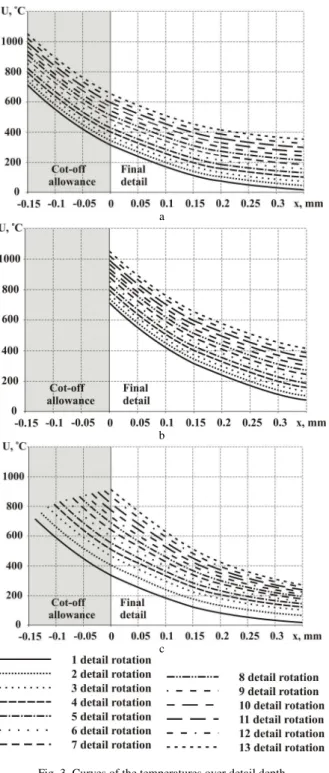
Heating temperature fields for steel working piece grinding cycle were calculated per generated model. Fig. 3 presents three variants of curves for temperature distribution over machined detail depth at each working piece rotation under similar machining conditions: D=100 mm;

Vsrad=1.015 mm/min; nw=88 rpm; 2A=0.3 mm. Fig. 4 shows temperature field on machined surface, corresponding to the first calculation variant (Fig. 3a).

For the first variant temperatures calculation was performed taking into account total cut-off allowance, i.e. calculation is performed from the working piece surface. In this case temperature on the working piece surface becomes a criterial (burning) temperature, leading to high reserve over maximum overheating of the final detail surface layer (Fig. 3a). Temperature curves, presented at Fig. 3b, are obtained during calculation, not taking into account cut-off allowance, i.e., based on final detail surface. In this case criterial temperatures exceed burning temperature (800 ° ), leading to necessity of correcting cutting modes to the downside.

Third variant of temperature curves (Fig. 3c) reflects actual process of allowance cutting-off for the grinding cycle under constant feed speed. We can see that under taken technological conditions final detail surface will remain defects free at first ten working piece rotations, and on the last three rotations surface temperature will overcome limiting temperature, making cutting modes corrections necessary.

V. CONCLUSIONS

Performed analysis for three calculation variants per generated feed model has demonstrated that third method (when feed is recalculated at each following detail rotation for the whole machining cycle) is most effective.

It is also not possible to assure heat defects absence in case, when temperature is determined for the final detail surface, not taking into account allowance changing during machining.

ISBN: 978-988-14047-2-5

(4)

We've found that temperature of the machined surface is not a sufficient condition for determining defects-free cutting modes when designing grinding cycle, as it does not take into account allowance, cut-off during machining.

So varying cutting modes over machining cycle, namely feed increasing in the beginning of machining cycle and decreasing when approaching final detail surface, while fulfilling requirement on burn-free machining, is one of the main directions of grinding effectiveness increasing.

Generated thermo physical model allows calculating temperature fields in processed detail, taking into account materials parameters, tolerance, cut off at each work piece turn, acting heat source duration and intensity at each work piece turn, and heat dissipation to process fluid, allowing forming multistep heavy-duty grinding cycles.

Now we are working on generating models of process limitations per processing accuracy, roughness, residual stresses, etc., as well, as on complex combing them with thermo-physical model. Complex model will allow forming multi-step heavy duty grinding cycles under following full range of process limitations, taken into account for producing specific detail.

REFERENCES

[1] Cutting Modes for Operations, Performed on Grinding and Finishing Manually and Semiautomatically Controlled Machines. Guide Book. Chelyabinsk: ATOKSO printing house, 2007.

[2] General Machine-Building Regulations on Cutting Modes for Technical Regulating of Operating Grinding Finishing Machines. Moscow: NIItruda, 1967.

[3] General Machine-Building Regulations on Cutting Modes for Technical Regulating of Operating Metal Cutting Machines.Part 3: Broaching, Grinding, and Finishing Machines. Moscow: Printing House of the Central Office for Scientific and Technical Information, 1978.

[4] General Machine-Building Regulations on Time and Cutting Modes for Regulating Works, Performed on Multipurpose and Universal Machines with Numerical Control. Part 2: Cutting Modes Rules. Moscow: Economika Publ., 1990.

[5] P. Krajnik, R. Drazumeric, J. Badger and F. Hashimoto, “Cycle Optimization in Cam-lobe Grinding for High Productivity,” CIRP Annals – Manufacturing Technology, 2014, vol. 63, pp. 333-336. [6] I. Gallego, “Intelligent Centerless Grinding: Global Solution for

Process Instabilities and Optimal Cycle Design,” CIRP Annals – Manufacturing Technology, 2007, vol. 56, no. 1, pp. 347-352. [7] P. Krajnik, R. Drazumeric and J. Badger, “Optimization of

peripheral non-round cylindrical grinding via an adaptable constant-temperature process,” CIRP Annals – Manufacturing Technology, 2013, vol. 62, pp. 347-350.

[8] D. Barrenetxea, J. Alvarez, J. Marquinez, I. Gallego, I.M. Perello and P. Krajnik, “Stability analysis and optimization algorithms for the set-up of infeed centerless grinding,” International Journal of Machine Tools & Manufacture, 2014, vol. 84, pp. 17-32.

[9] G.B. Lurie Progressive Methods of Round External Grinding. Leningrad: Mashinostroenie Publ., 1984.

[10] P. Comley, I. Walton, T. Jin and D.J. Stephenson, “A High Material Removal Rate Grinding Process for the Production of Automotive Crankshafts,” CIRP Annals – Manufacturing Technology, 2006, vol. 55, no. 1, pp. 347-350.

[11] D.E. Anel'chik, “Cycles of Defects-free Machining on Grinding Machines,” Metal Cutting Machines; Republic Interdisciplinary Scientific and Technical Collected Book, 1989, vol. 17, pp. 68-71. [12] J. Peters and R. Aerens, “Optimization Procedure of Three Phase

Grinding Cycles of a Series without Intermediate Dressing,” Annals of the CIRP, 1980, vol. 29, no. 1, pp. 195-200.

[13] S. Malkin, “Grinding Cycle Optimization,” Annals of the CIRP, 1981, vol. 30, no. 1, pp. 223-226.

[14] B. Rowe, Principles of Modern Grinding Technology. Norwich: Andrew Publishing, 2009.

[15] A. D`yakonov, “Blank-cutter interaction in high-speed cutting,” Russian Engineering Research, vol. 34, Is.12, 2015, pp. 775–777. [16] A. D`yakonov, “Effective Cutting Conditions in Abrasive

Mashining,” Russian Engineering Research, vol. 34, Is.12, 2015, pp. 778–780.

a

b

c

Fig. 3. Curves of the temperatures over detail depth a – taking into account total cut off allowance;

b – not taking into account cut off allowance; c – taking into account allowance, cut off per each detail rotation

Fig. 4. Temperature field on the machined surface in grinding cycle (first 10 working piece rotations)

ISBN: 978-988-14047-2-5