A.N. Kolmogorov’s defence of Mendelism
Alan Stark and Eugene Seneta
School of Mathematics and Statistics, University of Sydney, Sydney, Australia.
Abstract
In 1939 N.I. Ermolaeva published the results of an experiment which repeated parts of Mendel’s classical experi-ments. On the basis of her experiment she concluded that Mendel’s principle that self-pollination of hybrid plants gave rise to segregation proportions 3:1 was false. The great probability theorist A.N. Kolmogorov reviewed Ermolaeva’s data using a test, now referred to as Kolmogorov’s, or Kolmogorov-Smirnov, test, which he had pro-posed in 1933. He found, contrary to Ermolaeva, that her results clearly confirmed Mendel’s principle. This paper shows that there were methodological flaws in Kolmogorov’s statistical analysis and presents a substantially ad-justed approach, which confirms his conclusions. Some historical commentary on the Lysenko-era background is given, to illuminate the relationship of the disciplines of genetics and statistics in the struggle against the prevailing politically-correct pseudoscience in the Soviet Union. There is a Brazilian connection through the person of Th. Dobzhansky.
Key words:Mendel’s peas, hybrids, segregation ratio, Kolmogorov-Smirnov test, chi-squared test.
Received: November 26, 2010; Accepted: December 21, 2010.
Introduction
Kolmogoroff (1940) [note that in bibliographies mogorov’s name is frequently cited and spelled as Kol-mogoroff; as also done herein, whenever references are given] analysed two tables, Tables 4 and 6 of Ermolaeva (1939), who summarized and analysed the results of a se-ries of experiments which she had done in the preceding years. Ermolaeva followed the design of some experiments made by Mendel (1866), in what may be seen now as a pointless exercise, to disprove Mendel’s principal law of inheritance. Nowadays every basic course of biology states that if one observes self-pollination of a hybrid plant the proportion of dominant plants grown from the resultant seeds will be 3/4.
The main part of Ermolaeva’s data related to colour of seed coat: whitevs.greyish-brown, correlated with white
vs.violet flowers (Ermolaeva’s Table 4) and colour of coty-ledons: yellow or green (Ermolaeva’s Table 6). The domi-nant states are respectively grayish-brown seed coat and yellow cotyledon. Ermolaeva did extensive experiments on colour of the seed coat and colour of the seed cotyledon.
Ermolaeva said that her data did not support a model of a constant underlying proportion and in this she was sup-ported by Lyssenko (1940) [note that Lysenko’s name frequently appears as Lyssenko in the literature] who there-fore concluded that Kolmogorov was wrong. But
Kolmo-goroff (1940) wrote: “This material, despite Ermolaeva’s claims to the contrary, has proved to be a new brilliant con-firmation of Mendel’s laws.” Kolmogorov’s paper is inter-esting for a number of reasons: it appeared at a critical time for the discipline of genetics in the Soviet Union but also it was an early example of the application of his own statisti-cal test (Kolmogoroff, 1933).
LetSn(x) denote the empirical distribution function of a simple sample of sizendrawn from a population in which the random variableXhas a continuous distribution func-tionF(x). That isSn(x) =N(x)/n, whereN(x) = number of sample values£x. Denote byDnthe supremum over the full range ofxof |Sn(x) -F(x)|. Kolmogoroff (1933) gave the limit distribution of the random variableDn, giving an ex-pression for the limiting form asn® ¥of Pr(Dn < l/ n) for arbitrary positivel. SinceDntends to zero asn® ¥, Kolmogorov’s formula provides the basis of a test that a sample of values ofXcome from a postulated distributionF
providingnis large. The limiting expression is given in our third section.
The main part of this paper examines Kolmogorov’s application of his test to Tables 4 and 6 of Ermolaeva (1939) following a section on the data itself. We reproduce the relevant columns of these two tables as our Tables 4 and 5 respectively. Ermolaeva (1939) concluded that her exper-iment proved that self-pollination of hybrids,AaxAa, did not produce a consistent segregation ratio. The second is-sue, assuming that there is a consistent ratio, is whether the proportion of dominants is 3/4. The fourth section of this www.sbg.org.br
Send correspondence to Eugene Seneta. School of Mathematics and Statistics, FO7, University of Sydney, NSW 2006 Australia. E-mail: [email protected].
paper uses a partition ofc2to analyse both issues. Some his-torical background is given in the fifth section and some general comments in the final section.
Ermolaeva’s Experiment
Ermolaeva’s Table 4 consists of 98 entries relating to seed coat colour. It appears that each entry gives the num-bers of dominant and recessive plants (or potential plants, if grown) produced by a single hybrid plant. Thus, Table 4 providesn= 98 sample values. The variate of interest is the observed proportion of dominants and so the binomial dis-tribution provides the model of variation. Kolmogorov ex-ploited the normal as an approximation to the binomial distribution. Table 5 provides 122 values relating to colour of cotyledon.
A question raised by Kolmogoroff (1940) concerned the numbers of plants in each family, that is in each line of Tables 4 and 5, and hence of the validity of using the stan-dard normal distribution as a model of the binomial. Taking 20 as a desired minimum number of seeds (justification in our Section 4), it is seen that the data relating to seed-coat colour are not satisfactory: only a small number of families have number of seeds of 20 or more. The summary details for Table 4 are: minimum number 2, first quartile 9, median 11.5, third quartile 17, and maximum 33. The numbers in respect of cotyledon colour are more satisfactory: mini-mum 6, first quartile 16.25, median 22, third quartile 28.75, maximum 64. Clearly the use of Kolmogorov’s test given below is easier to justify in respect of cotyledon colour.
In the light of the low counts in many families, there would be many observed proportions varying markedly from Mendel’s proportion 3/4. Also, in view of experience obtained from experiments before and after Ermolaeva’s, some of the results obtained could be explained only as re-sulting from technical errors such as a parental plant being homozygotic rather than hybrid.
Table 1 of our paper is a reproduction of part of Ermolaeva’s Table 3 which relates to cotyledon colour. Her Table 3, closely related to the data in her Table 6 (our Ta-ble 5), but not entirely to only this data, gives the lines used to obtain the hybrid seeds, reference numbers to sets of pollinations, the numbers of plants in a set, the number of seeds classified as dominant, the number recessive, the per-centage of seeds dominant and Ermolaeva’s indication of goodness of fit to Mendel’s 3:1 model, poor fit being de-noted by the symbol ‘P’. Some of the indications of signifi-cance in Ermolaeva’s tables are based on far more stringent requirements than are customary. For example, the very first entry in our Table 1 is marked as significant when the observed number of dominants differs from expected by about one standard error.
Table 2 of Ermolaeva, closely related to the data in her Table 4, but not entirely to only this data, is reproduced here as our Table 2, and gives a list of the lines used to
ob-tain the hybrid seeds used to study seed-coat colour. It sum-marises the numbers of dominant and recessive forms ob-tained from individual seeds. Data in Ermolaeva’s Table 5 relating to seed form were obtained from only 5 plants and are not considered here. Ermolaeva (1939) noted one item of detail: “We did not have the opportunity to cross the same pair of plants several times, due to the fact that peas have a comparatively low number of flowers and for a short period of time. Because of this we took several pairs of the
Table 1- Segregation of cotyledon colour.
Crossing Ref #Plants #Dom #Rec %Dom Fit†
179a x 47 1 8 157 44 78.1 P
179a x 47 2 7 120 44 73.2
179a x 47 3 4 42 27 60.9 P
179a x 47 4 6 99 43 69.7 P
179a x 47 5 11 135 59 69.6 P
6 x 47 6 8 119 37 76.3
6 x 47 7 7 116 37 75.8
178 x 47 8 9 153 47 76.5
178 x 47 9 11 208 69 75.1
178 x 47 10 10 170 54 75.9
178 x 47 12 11 159 68 70.0 P
178 x 47 13 10 175 63 73.5
178 x 47 14 8 122 40 75.3
178 x 47 15 7 190 69 73.4
178 x 47 16 6 58 44 56.8 P
†The symbolPmarks counts which Ermolaeva regarded as inconsistent with Mendel’s model.
Table 2- Segregation of seed-coat colour.
Crossing Ref #Plants #Dom #Rec %Dom Fit†
128 x 47 1 3 48 12 80.0
128 x 47 2 5 40 24 62.5 P
128 x 47 6 6 64 28 69.6 P
128 x 47 9 10 110 38 74.3
128 x 47 10 12 129 37 77.7
6 x 47 3 9 50 24 67.6 P
702 x 47 4 6 74 31 70.5 P
702 x 47 5 4 19 7 73.1
702 x 47 7 10 74 40 64.9 P
702 x 47 8 9 94 18 83.9 P
702 x 47 11 8 75 21 78.1
702 x 47 12 8 45 26 63.4 P
702 x 47 13 10 102 33 75.6
702 x 47 13a 7 84 16 84.0 P
same pure-bred types of peas.” Fisher (1936) noted that on average about 30 seeds were classified from each plant in some of Mendel’s experiments. As can be seen from Tables 1 and 2 of the present paper, on average fewer [than 30] seeds were classified from each mother plant in Ermo-laeva’s experiment.
Tables 1 and 2 of this paper show that the same paren-tal line (47) was used in the production of all hybrids of the two characters. Ermolaeva did not indicate which line was used as the mother plant from which the F1 seeds were
taken. It may be that she followed Mendel in making the cross in both reciprocal directions.
Summing the numbers in Table 1 yields 2023 domi-nant and 745 recessive seeds so that the percentage of dominants is 73.1%. The standard error of the observed proportion assuming hypothetical value 0.75 and number of seeds 2023 + 745 = 2768 is 0.00823. Dividing the differ-ence of the observed proportion from 0.75 by the standard error gives an approximate standard normal value 2.326. The two-sided probability of exceeding this value is ap-proximately 2%.
Summing the numbers in Table 2 yields 1008 domi-nant and 355 recessive seeds so that the percentage of dominants is 74.0%. The standard error of the observed proportion assuming hypothetical value 0.75 and number of seeds 1008 + 355 = 1363 is 0.01173. Dividing the differ-ence of the observed proportion from 0.75 by the standard error gives an approximate standard normal value 0.891. The two-sided probability of exceeding this value is ap-proximately 37%.
There are many discrepancies between Ermolaeva’s Tables 4 and 6 and the earlier tables.
Rather than referring to the vast amount of work car-ried out elsewhere which overwhelmingly supported Men-del’s, Ermolaeva (1939) included a quotation from the Ly-senko-era geneticist Lev Nikolaevich Delone (Delaunay) (1891-1969). Delone had established a reputation in the So-viet Union using radiation to induce mutations in wheat. He adopted the usual rhetorical device of attributing to the Mendelians something which they would not use in prac-tice. In this case it concerned a plan to produce a plant with a desirable trait or combination of traits controlled by a large number of recessive genes. Delone stated that the probability of obtaining a plant with the desired character-istic from hybrids is 4-n, wherenis the number of independ-ent (unlinked) genes controlling the trait. Whennis large, the correctness of this formula is precisely the reason why a Mendelian would not use a mass planting in the hope of finding a plant with the desirable combination of traits.
At least, when referring to orthodox geneticists, Er-molaeva did not use the pejorative label “Johannsen-Men-delian-Morganist”, or the more usual label in which Weis-mann replaces Johannsen, as was Lysenko’s custom. At the core of the disagreement between Lysenko and his puppet master Stalin on one side and orthodox geneticists on the
other was the concept summarized by Wright (1917): “He-redity as looked upon since the time of Weismann is relatively simple to understand. It consists merely in the persistence of a certain cell constitution (in the germ cells) through an unending succession of cell divisions.” Lysenko (1951) claimed, for example, that geneticists believed that this meant that the development of plants and animals was not affected by environmental factors and that the germ plasm could not be changed by mutation. Lysenko either did not understand, or simply ignored, the fact that geneti-cists recognized the presence of heterozygosity, when it was there, and exploited it in selection for desirable traits, just as he did not understand the possible existence of ‘pure lines’, such as those studied by Johannsen.
The marked disparity between the numbers of seeds obtained to study seed-coat colour and those for colour of cotyledon was noted above. Families number 4 and 38 in Table 4 have rather low numbers of dominant seeds. These two features suggest that there may have been problems in the conduct of these experiments. Family 41 in Table 5 (Ermolaeva’s Table 6) also has a very low number of dominants.
Kolmogorov’s Analysis
Taking Mendel’s model of hybrid heterozygosity Kolmogorov gives the binomial probability of observingm
dominants innoffspring:
P m n
m n m n
m n m
( ) ! !( )! = -æ è ç ö ø ÷ æ è ç ö ø ÷ -3 4 1 4 (1)
Kolmogorov then recommends that, if the number of individuals in each family is very low, for example less than 10, it is feasible to verify formula (1) with the aid of “thec2 criterion of [Karl] Pearson”. He does not elaborate on this suggestion. It may be a mistranslation into English of Kol-mogorov’s intentions, by his translator.
He then defines the normalized deviationsDas
D =æ -è
ç ö
ø
÷ =
m
n n n n
3 4
3 4
:s ,where s (2)
and notes that these normalized deviationsDobey approxi-mately the “law of Gauss with unit dispersion”, that is the probability for the inequalityD £xto hold is approximately equal to
P x e d
x ( )= - / -¥
ò
1 2 2 2 p x x (3)propor-tion of families showing |D| > 1 should be regarded as dis-proving Mendel’s theory.”
Kolmogorov then makes a formal analysis of Ermolaeva’s experiments by means of the what is now known as Kolmogorov’s test, which is a one-sample ver-sion of the later Kolmogorov-Smirnov two-sample test. He takes the sets of standardized values (2) and tests them against the standard normal distribution.
He refers to the account of his own test , introduced in Kolmogoroff (1933), as presented in the monograph of the leading Russian mathematical statistician of his time, Romanovsky (1938). In this book, the relevant material oc-curs on pp. 226-229 (Kolmogorov cites p. 226) in a section whose title (in English translation) is: 61.A new criterion for agreement of an empirical and a theoretical distribu-tion. Kolmogoroff (1940) uses the notationF(l), of the book, in the way we describe below. We note also that in the preceding section of his book, Romanovsky (1938) uses thec2goodness of fit criterion of Karl Pearson to illustrate the same example as in his Section 61. It is also relevant that Kolmogorov had reviewed the book of Romanovsky (1938) when it had appeared, so he would have had it to hand when composing, in the guise of mathematical statis-tician, the note Kolmogoff(1940).
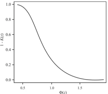
The following is an adaptation from p. 450 of Gnedenko (1968), a close associate of Kolmogorov, of di-rections for the use of Kolmogorov’s test. If the cumulative distribution function under testF(x) is continuous and the empirical distribution function from a sample of sizenis denoted byFn(x), then asn® ¥,
Pr( nDn £l)®K( )l =0, for l£0
= - - >
=-¥ ¥
å
( 1)k 2k2 2 0.k
e l for l
If the number of trials is very large, then
Pr( nDn £l)=K( ) (l approximately .)
LetDn(0)denote the maximum value of |Fn(x) –F(x)| actually found, and setl0=ÖnDn(0). If the difference
F(l0)= -1 K(l0)= -1 Pr( nDn £l)approximately
is sufficiently small (conventionally, less than 0.05), then a very unlikely event has occurred, and the difference
be-tweenFn(x) andF(x) is regarded as significant and no lon-ger explained by the randomness of the observed values. However, if F(l0) is large, then the difference between
Fn(x) andF(x) is considered insignificant, and our hypothe-sizedF(x) may be regarded as being compatible with exper-iment. Figure 1 displays the functionF(l)for values ofl from 0.4 to 1.5. Note thatnis used in two senses in quoting from Kolmogorov’s paper and Gnedenko’s monograph. In the formernis used as the number of seeds or plants in a ‘family’ and in the latter the number of lines in either Table 4 or 6 of Ermolaeva, that is the sample size in Kolmo-gorov’s test.
Kolmogorov’s values forl0were respectively 0.75,
F(l0) = 0.37 for colour of cotyledon (Table 5, 122
fami-lies); and 0.82, F(l0) = 0.49 for colour of seed coat
(Table 4, 98 families). Thus, according to these values, agreement in both cases is good: and on p. 41, Kolmogoroff (1940) describes it as “quite satisfactory”.
We attempted to verify Kolmogorov’s calculations using the statistical packageR, specifically its procedure
ks.test, relevant to the Kolmogorov-Smirnov tests, on the obtained frequencies in Tables 4 and 6, reproduced here in condensed form in Tables 4 and 5 respectively. For colour of cotyledon the criterion of maximum difference between empirical and theoretical distribution functionDn= 0.0905
Figure 1- Graph ofF(z) = 1 -K(z).
Table 3- Extract from Kolmogoroff (1940).
Segregation for the colour of the flower and axil
Segregation for the colour of cotyledons
Theoretically expected
% % %
Total number of families 98 100 123 100 100
showing |D|£1 66 67 85 69 68
andl0= 0.999, with 2-sided probability 0.27 and for
seed-coat colourDn= 0.0667 andl0= 0.660, with probability
0.78. Our Figure 2 shows the empirical distribution of val-ues relating to colour of cotyledon plotted against the stan-dard normal distribution function and Figure 3 the corre-sponding plots for seed-coat colour. A notable feature of both Figure 2 and Figure 3 is the negative skewness of the distributions of proportions.ks.testadvised that the proba-bilities shown above which it calculated were not correct because of the presence of coincidences in the data sets.
Figures 2 and 3 give a visual impression of agreement with the Mendel model except at the left hand end. Gne-denko (1968), however, clearly specifies that the test was to be applied to continuous distributions whereas the data in this application are discrete, and there are some duplica-tions of values of both sets of data, an event which has zero probability for continuous distributions. Accordingly there are ambiguities in calculating the probability associated with maximumDnvalues.
A related problem is inclusion in the above analysis of small families, whereas forDto properly approximate a
sample value from a standard normal distribution, the fam-ily sizenshould be large. In respect of seed-coat colour, for example, there are two plants with 2 dominant and 3 reces-sive seeds. These were the readings associated with maxi-mumDnvalue. In respect of colour of cotyledon, the maxi-mum Dn occurred at cumulative probability around 0.5. Additionally, in Table 5 there are some suspect readings. Family # 148 records 0 dominants and 10 recessives, while family # 105 records 50 dominants and 0 recessives. In Ermolaeva’s Table 4, there is one plant from which all seeds were classified as recessive. Such readings are highly unlikely results from hybrid crossesAaxAa.
Analysis of Ermolaeva’s Tables 4 and 6 Using
the Chi-Squared Distribution
A rule of thumb which is generally applied in the re-lated statistical problem of applying a normal approxima-tion with continuity correcapproxima-tion to readings from a binomial distribution is that bothnp³5 andn(1 - p)³5, wherep
(here 3/4), is the probability of “success” inntrials. Thus if we apply this rule, family size should be at least 20. If we
Table 4- Condensed version of Ermolaeva’s Table 4.
Set Fam. D : r Set Fam. D : r Set Fam. D : r Set Fam. D : r
1 1 17 : 3 5 26 7 : 1 8 52 3 : 2 11 77 13 : 3
1 2 16 : 4 5 27 5 : 0 8 53 7 : 4 11 78 7 : 5
1 3 15 : 5 6 28 17 : 6 9 54 14 : 3 11 79 14 : 3
2 4 11 : 11 6 29 4 : 6 9 55 17 : 7 11 80 3 : 1
2 5 4 : 5 6 30 12 : 4 9 56 14 : 2 11 81 12 : 3
2 6 8 : 3 6 31 8 : 3 9 57 16 : 4 11 82 6 : 3
2 7 10 : 3 6 32 15 : 4 9 58 14 : 3 12 83 8 : 4
2 8 7 : 2 6 33 8 : 5 9 59 7 : 1 12 84 12 : 4
3 9 4 : 2 7 34 5 : 2 9 60 9 : 1 12 85 9 : 5
3 10 9 : 1 7 35 5 : 3 9 61 10 : 7 12 86 5 : 2
3 11 3 : 7 7 36 12 : 5 9 62 12 : 6 12 88 2 : 1
3 12 6 : 3 7 37 6 : 1 10 63 15 : 4 12 89 4 : 3
3 13 10 : 2 7 38 18: 13 10 64 5 : 1 12 90 5 : 6
3 14 2 : 3 7 39 4 : 1 10 65 11 : 5 12 91 9 : 4
3 15 10 : 1 7 40 3 : 2 10 66 2 : 0 13 92 15 : 3
3 16 2 : 3 7 41 5 : 1 10 67 21 : 8 13 93 23 : 3
3 17 4 : 2 7 42 8 : 8 10 68 13 : 5 13 94 8 : 1
4 18 11 : 6 7 43 8 : 4 10 69 8 : 3 13 95 8 : 1
4 19 7 : 4 8 44 15 : 3 10 70 17 : 1 13 96 13 : 2
4 20 26 : 7 8 45 7 : 2 10 71 13 : 3 13 97 0 : 17
4 21 12 : 7 8 46 23 : 3 10 72 9 : 2 13 98 10 : 0
4 22 14 : 4 8 47 12 : 1 10 73 5 : 1 13 99 9 : 0
4 23 6 : 3 8 48 18 : 3 10 74 10 : 4 13 100 7 : 2
5 24 4 : 3 8 49 11 : 0 11 75 11 : 3
5 25 3 : 3 8 51 8 : 2 11 76 9 : 0
apply this rule by including only families of at least 20, and additionally exclude from consideration from Table 5 fam-ily # 105, we can be reasonably confident that eachD2, the square of a standard normal variable, has ac2distribution independently of the otherD2’s, and when we sum such D2
’s, the sum will have acN2distribution, whereNis the number of summands, under the hypothesis the Mendelian “3/4”.
Then for Table 4 we obtain observedc132= 20.579,
with p-value a 0.09; and for her Table 6c752= 90.211, with
p-value 0.11. Since both p-values exceed the conventional
cut-off of 0.05, there is no strong statistical evidence against the Mendelian hypothesis.
In the above briefc2analysis we have attempted to use an essentially equivalent test to Kolmogorov’s inas-much as it relies on the approximate standard normality of theD’s, after “cleaning” the data appropriately. So while the conclusion drawn by Kolmogoroff (1940) confirms what is now totally accepted, the evidence in support of this conclusion is not as strong as his paper presents. Of course his statistical technology was well beyond the understand-ing of Lyssenko (1940) and Kolman (1940), who could hardly argue on the grounds of its incompletely justified ap-plication and possible arithmetic error, to data which may have been poorly prepared. Seneta (2004) describes Kol-man’s leading role in the attacks on mathematicians and traditional pure mathematics in the Soviet Union during the Stalinist era.
We now pass to a consideration of Ermolaeva’s Ta-bles 2 and 3 (our TaTa-bles 2 and 1 respectively). These at first appear to be condensations of Tables 4 and 6, and while this is partially true, there are a number of inconsistencies and inaccuracies.
For example the third line of Table 1 should show 52 dominants instead of 42. Making the substitution in that line gives the percentage of dominants as 65.8 instead of 60.9.
There are 122 lines of data in Table 5, but there are 123 families considered in Table 1. Kolmogoroff (1940) therefore thought the number of lines in Table 5 was 123 while it is actually 122. He reports 38 as the number of lines in Table 5 whereD > 1, which is correct, but the percentage is slightly “out”, since it relates to a total of 123.
Each line in Table 5 appears to be the result of scoring the state, that is with either yellow or green cotyledon, of the seeds from the pod or pods produced by a self-pol-linating hybrid plant derived from the pollination desig-nated in Table 1.
It seems that some hybrid plants produced one use-able or used pod and others more. Summing the numbers in Table 6 yields 2104 dominants and 742 recessives, the per-centage of dominants 73.9 and a standard normal value 1.320, so not significantly different from 3/4.
Looking at the histogram of the 122 individual pro-portions of dominants gives only weak support to the view taken by Lyssenko (1940), discussed below, that it is not reasonable to consider that the segregation of states comes from a single underlying proportion 3/4, but rather that the phenomenon is more variable. There are 13 proportions be-low 0.6, some clearly explicable by virtue of small sample size. The final entry gives 10 seeds all recessive. This was part of batch 16 (Table 1), which was one of 8 batches of the cross 178 x 47. Table 1 shows that the other 7 batches gave proportions remarkably consistent with 3/4. Ermolaeva shows 6 plants used in batch 16 (Table 1) whereas there are
Figure 2- Empirical cumulative distribution function ofDvalues (—) re-lating to colour of cotyledon plotted against the standard normal distribu-tion funcdistribu-tion (....).
only 5 in Table 5. Summing these five yields the percentage 59.8 instead of the 56.8 given by Ermolaeva.
Ermolaeva constructed her Table 2 by condensing the data relating to colour of the seed-coat given in Table 4. About one third of the lines in Table 2 are inconsistent with the entries in Table 4. There are 98 lines of data in Ermo-laeva’s Table 4. The total number of dominants is 939 and recessives 336 giving the percentage of dominants 73.6 and standard normal value 1.116. The final line of Table 2 gives a batch with label 13a for which there are no corresponding entries in Table 4. This accounts for much but not all of the difference between the total numbers of plants of the two tables.
Fisher (1924) and associated papers examine the pro-perties of the formula developed by Pearson (1900)
c2
2
= æ -è
çç ö
ø ÷÷
S x m
m
( )
, (4)
whereSdenotes summation over a number of cell frequen-cies,xis a typical cell count andmthe corresponding ex-pected cell count. Consider a single line in Ermolaeva’s Table 4 (or 6) and denote bydthe number of ‘dominants’, byrthe number of ‘recessives’ and byqthe expected pro-portion of dominants. Because
( ( ))
( )
( ( )( ))
( )( )
( (
d d r
d r
r d r
d r
d d
- +
+ +
- - +
- + =
-q
q
q q
q
2 2
1 1
+
- +
r d r
))
( )( )
2
1
q q (5)
the refinements demonstrated by Fisher can be applied to D2
as defined in (2) and sums of such terms. Fisher (1924)
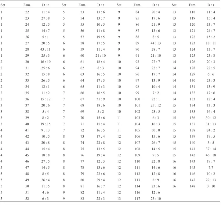
Table 5- Condensed version of Ermolaeva’s Table 6.
Set Fam. D : r Set Fam. D : r Set Fam. D : r Set Fam. D : r
1 22 11 : 4 5 53 13 : 6 9 84 20 : 4 13 118 11 : 4
1 23 27 : 8 5 54 13 : 7 9 85 17 : 6 13 119 15 : 4
1 24 12 : 5 5 55 10 : 5 9 86 21 : 9 13 120 13 : 7
1 25 14 : 7 5 56 11 : 8 9 87 13 : 6 13 121 24 : 7
1 26 5 : 1 5 57 19 : 5 9 88 8 : 5 13 122 15 : 2
1 27 20 : 5 6 58 17 : 5 9 89 44 : 13 13 123 18 : 11
1 28 43 : 11 6 59 11 : 4 9 90 28 : 7 13 124 13 : 7
1 29 25 : 3 6 60 21 : 10 9 91 21 : 10 13 125 23 : 8
2 30 16 : 10 6 61 18 : 4 10 93 27 : 7 14 126 20 : 3
2 31 25 : 6 6 62 8 : 3 10 94 22 : 7 14 128 22 : 5
2 32 15 : 8 6 63 16 : 5 10 96 17 : 7 14 129 6 : 6
2 33 26 : 5 6 64 17 : 3 10 97 13 : 9 14 130 23 : 3
2 34 12 : 1 6 65 11 : 3 10 98 10 : 4 14 131 13 : 9
2 35 11 : 2 7 66 16 : 5 10 99 7 : 2 14 132 17 : 6
2 36 15 : 12 7 67 31 : 9 10 100 22 : 1 14 133 12 : 4
3 37 20 : 6 7 68 18 : 6 10 101 25 : 12 15 134 13 : 3
3 38 5 : 4 7 69 5 : 2 10 102 23 : 5 15 135 16 : 4
3 39 8 : 2 7 70 15 : 6 11 103 6 : 3 15 136 30 : 12
3 40 19 : 15 7 71 15 : 4 11 104 16 : 3 15 137 31 : 13
4 41 9 : 13 7 72 16 : 5 11 105 50 : 0 15 138 24 : 2
4 42 10 : 5 8 73 17 : 4 12 106 15 : 6 15 139 19 : 5
4 43 20 : 8 8 74 22 : 8 12 107 26 : 7 15 140 3 : 5
4 44 15 : 4 8 75 13 : 5 12 108 14 : 5 15 141 37 : 14
4 45 18 : 8 8 76 19 : 4 12 109 9 : 5 15 142 46 : 18
4 46 27 : 5 8 77 12 : 3 12 110 22 : 8 16 143 19 : 7
5 47 14 : 5 8 78 13 : 6 12 111 14 : 6 16 145 7:7
5 48 8 : 5 8 79 22 : 6 12 112 12 : 8 16 146 10 : 2
5 49 26 : 4 8 80 29 : 4 12 113 8 : 9 16 147 22 : 13
5 50 11 : 5 8 81 16 : 7 12 114 23 : 6 16 148 0 : 10
5 51 4 : 6 9 82 11 : 4 12 116 12 : 6
5 52 6 : 3 9 83 22 : 3 13 117 23 : 10
set out the conditions which should apply when using (4) as a “measure of discrepancy between observation and expec-tation”. An important issue in the application of (4) is using the correct number of degrees of freedom. Fisher noted that these should be determined by the number of degrees of freedom in which observation and expectation might differ. So, in applying (4) to (5), although there are 2 cells there is only one degree of freedom, in accord with the use ofD2 earlier. Fisher noted that, if an estimate~q ofqwas made, the number of degrees of freedom should be reduced by one. Further, such an estimate should be consistent and effi-cient and an estimate made by minimisingc2was both. The left hand side of (5) and therefore the equivalent right hand side can be applied to Tables 4 and 6 by substitutingq= 3/4 withNdegrees of freedom andq q=~, withN- 1 degrees of freedom. The difference between the two values ofc2isc2 with one degree of freedom and measures the improvement to the goodness of fit made by estimatingqfrom the data. It also provides a test of whetherq= 3/4 should be rejected.
The estimate~q =0 740 is obtained from the reduced. data set of Table 4 with c122 = 20.401 (p = 0.074) and
c12= 0.178 (p = 0.95). The corresponding values obtained
from the reduced data set of Table 5 are ~q =0 7365,. c742= 88.051 (p = 0.14) andc12= 2.160 (p = 0.36).
Accord-ingly, in neither case does~q provide a significantly better fit to the data than 3/4.
Some Historical Background
Sheynin (2001),in his Section 6.Genetika gives an account of the fate of Mendelian genetics in the Soviet Un-ion in the 1930’s and 1940’s. Here without his specific cita-tions are extracts in translation by one of the authors (ES) as well as supplementary information from Sheynin (2008):
Up to 1930, the USSR was “the leading cen-tre for investigations of Mendelianism and was ac-knowledged as such worldwide” ... but from 1939 the development of Soviet genetics was blocked, and in 1948 it was totally destroyed. From 1935 genetics was called an idealistic science in opposi-tion to dialectical materialism, and N.I. Vavilov, its foremost figure, began to be persecuted...He was arrested in 1940,and died in prison in 1943.
The final destruction of genetics occurred in 1948 at the All-Union conference...the main perse-cutor being T.D. Lysenko. ...At this conference V.S. Nemchinov also participated. His speech was repeatedly interrupted by loud jeers. Nevertheless he managed to say that “the chromosome theory of inheritance has entered the golden treasury of sci-ence”. And further: “I am able to verify this theory from the standpoint of... statistics.” At the Second All-Union Statistical Conference, of the same year [in Tashkent, Romanovsky’s home base -ES] he
was “decisively censured” for his attempts to statistically justify “reactionary Weismann-ist the-ories” and for his presentation “from positions of the Mach-ist Anglo-American School, which ac-cords statistics... the role of arbiter over other sci-ences.” It is not surprising that he soon had to leave his post as Director of the All-Union Timiriazev Agricultural Academy, and to resign as Chair of its Department of Statistics.
At the Tashkent Conference Romanovsky, the chairman of the organizing committee, who had been in correspondence with Nemchinov, had also to confess to “ideological errors, in some of his earlier work” [apparently as a result of his ad-herence to the direction of the English Biometric School of mathematical statistics – ES], even though Kolmogorov, who was present at the con-ference, in his report praised the great work done by Romanovsky and his School.
When the great probabilist S.N. Bernstein was about to publish the 5th edition of his textbook [Teoriia Veroiatnostei. (The Theory of Probabil-ity)] in 1949 or 1950 [the famous 4th edition had appeared in 1946 –ES], because he categorically refused to exclude a few pages dedicated to Men-delism, its publication was stopped at page-proof stage. It is not difficult to see that the censure at the Tashkent conference was a disguised censure of Kolmogorov [not least for his defence of Mende-lianism in Kolmogoroff (1940), with which Roma-novsky was associated – ES].
B.V. Gnedenko, perceiving that probability theory itself was beginning to come under attack as a result of their support, expressed regret [in 1950] at Kolmogorov’s and other leading mathemati-cians’ support of Mendelism; and with patience and reason tried to placate the Lysenko hotheads.”
The article by Ermolaeva (1939) was brought to Kol-mogorov’s attention (Kolmogoroff, 1940; footnote on p. 37) by the geneticist Aleksandr Sergeevich Serebrovsky (1892-1948), a dedicated “Morganist”. Kolman (1940) noted this motivation, and that he saw dangers in Sere-brovsky’s “errors” , of which “he more than once feigned to repent”. Kolman was a truly malign influence for Soviet science, in particular mathematical science (see Seneta, 2004) as well as biological. When he became the director of the Association of Natural Science of the Communist Aca-demy at the beginning of 1931, he:
Kolman (1940),on p. 836, as the “mathematical ex-pert” of the dialectical materialists, tries to harness S.N. Bernstein to his cause by citing a passage from the 1934 edition of the book of Bernstein:
“who writes that the results of crossing peas show compatibility with Mendel’s hypothesis. Now... compatibility neither proves nor confirms this theory, for the same material may prove to be compatible also with other theories.”
Kolman’s back-up note for Lyssenko (1940) was , of course, “Communicated by T.D. Lyssenko, Member of the Academy, 2.VII.1940”, as only Academicians had the right to publish or communicate in the Comptes Rendus (Do-klady). It must have been galling for Bernstein who is listed in the table of contents of the 30 September issue as
Rédacteur, though not chief editor; while Kolmogorov is one of theComité de Rédaction.
The information in the following three paragraphs sketches the genetic background to the paper by Kolmo-goroff (1940) and serves to introduce Dobzhansky’s role. It is extracted largely from Gaissinovitch (1980).
H.J. Muller brought cultures of AmericanDrosophila
from Morgan’s laboratory to Moscow in August 1922, and in the July 1927 issue ofSciencepublished a report of his research on the artificial production of mutations. Sere-brovsky succeeded in publishing an article in Pravda
(Number 207, September 11, 1927) in which he empha-sized not only the practical importance of Muller’s finding but also that they refuted the doctrine (Lamarckism) of the inheritance of acquired characteristics. As Senior Geneti-cist, 1933/1937, in Leningrad and Moscow, needless to say, Muller was heavily involved in the controversy with Ly-senko.
In fact, in 1926 the “Lamarckists” had issued a collec-tion of papers on the inheritance of acquired characteristics. Of the four essays, three defended the Lamarckian position and one, by the young Theodosius Dobzhansky (1900-1975), opposed it. This was before Muller’s important pub-lication on mutation. In 1927 Dobzhansky left Russia to work in Thomas Morgan’s laboratory in the USA. Morgan was to become one of the most reviled figures among Sta-linist biologists.
The Fifth International Congress of Genetics was held in Berlin in September 1927, and a large Soviet contin-gent participated. It included L.N. Delone, Iu. A. Filipchen-ko, A.S. Serebrovsky and N.I. Vavilov. S.S. Chetverikov (1880-1959) presented a major paper on his group’s (it had included Dobzhansky) work on wild populations of
Drosophila.
Chetverikov was arrested by the OGPU in 1929 and sent to Yekaterinburg for 5 years. He was dismissed in 1948 from his post through Lysenko’s influence.
Dobzhansky achieved great eminence for his work on
Drosophilaand played a prominent part in the “Evolution-ary Synthesis” which reconciled the theories of Mendel and
Darwin. He worked in Brazil and was well-known to prom-inent Brazilian geneticists of the day. Dobzhansky and Spassky (1959) give the site , year and collector of samples of Drosophila from various places in North and South America. Dobzhansky collected from Belem, July 1952; Ican, August 1952 and Angra dos Reis (state of Sao Paulo) in May 1956. Apart from these Brazilian sites he collected in several other sites in South America with C. Pavan in 1956. An earlier paper (Burla et al., 1949) includes as co-authors the distinguished Brazilian geneticists A.R. Cordeiro and C. Pavan. In Dobzhansky and Spassky (1959), Dobzhansky classified his samples in 6 groups : Centro American, Amazonian, Transitional (Colombia, Venezuela), Andean, Orinocan and Guianan. From the study of crossing flies from his samples, he concluded that “...D. paulistorumis, considered as a whole, a single spe-cies.’’ Dobzhansky’s influence is still evident in South America. Santos-Colares et al. (2006) cite the Burla et al.(1949) paper and note that the stocks used were collected by Dobzhansky and Pavan amongst others. Pavan and da Cunha (2003) give a much fuller account of Dobzhansky’s contributions to the advancement of genetics in Brazil.
Concluding Remarks
Fisher (1936) wrote: “In 1930, as a result of a study of the development of Darwin’s ideas, I pointed out that the modern genetical system, apart from such special features as dominance and linkage, could have been inferred by any abstract thinker in the middle of the nineteenth century if he were led to postulate that inheritance was particulate, that the germinal material was structural, and that the contribu-tions of the two parents were equivalent. I had at that time no suspicion that Mendel had arrived at his discovery in this way. From an examination of Mendel’s work it now ap-pears not improbable that he did so and that his ready as-sumption of the equivalence of the gametes was a potent factor in leading him to his theory. In this way his experi-mental programme becomes intelligible as a carefully planned demonstration of his conclusion.”
is concerned, this could be explained, at least in part, to lack of control. In respect of colour of cotyledon, as Kolman (1940) noted, the empirical distribution function lies fairly consistently to the left of the normal distribution function. But the same comment could not be made about seed-coat colour. In any case, taking into account the kinds ofa priori
considerations raised by Fisher, it would have been prudent to try to repeat the experiment and to move on to other ex-periments, for example to backcrossing, as Mendel did.
Acknowledgments
Alan Stark thanks Dr. Allen Dobrovolsky of A.D. Envirotech Australia Pty Ltd for translating Ermolaeva (1939) from Russian into English. Eugene Seneta thanks Dr. Thomas Fung, of Macquarie University, Sydney, for assistance with aspects of the statistical packageR. Both are grateful to Irene Buschtedt, Halyna Syta and Allen Dobrovolsky for finding electronic information concerning L.N. Delone.
References
Burla H, da Cunha AB, Cordeiro AR, Dobzhansky Th, Malo-golowkin C and Pavan C (1949) Thewillistonigroup of sib-ling species ofDrosophila. Evolution 3:300-314.
Delone LN (1936) Daet li chto-nibud’ “formal’naia genetika” dlia praktiki v’vedeniia novikh sortov? Sotsialistecheskaia Re-konstruktsiia Khozaistava, no. 12 [English translation of ti-tle : Does “formal genetics” give anything of value for the practice of introducing new varieties?].
Dobzhansky T and Spassky B (1959)Drosophila paulistorum, a cluster of speciesin statu nascendi. Proc Natl Acad Sci USA 45:419-428.
Ermolaeva NI (1939) Yeshche raz o gorokhovikh zakonakh. Ya-rovizatsiia – Zhurnal po Biologii Razvitiia Rastenii 2:79-86 [English translation of title: Once more on the “laws of peas”].
Fisher RA (1924) The conditions under whichc2measures the discrepancy between observation and hypothesis. J R Statist Soc 87:442-450.
Fisher RA (1936) Has Mendel’s work been rediscovered? Ann Sci 1:115-137.
Gaissinovitch AE (1980) The origins of Soviet genetics and the struggle with Lamarckism, 1922-1929. J Hist Biol 13:1-51. Gnedenko BV (1968) The Theory of Probability. 4th edition.
Chelsea Publishing Company, New York, 529 pp.
Kolman E (1940) Is it possible to prove or disprove Mendelism by mathematical and statistical methods? Dokl Akad Nauk SSSR 28:834-838.
Kolmogoroff A (1933) Sulla determinazione empirica di una legge di distribuzione. Giorn Ist Ital Attuari 4:83-91. Kolmogoroff AN (1940) On a new confirmation of Mendel’s
laws. Dokl Akad Nauk SSSR 27:37-41.
Lysenko TD (1951) The Situation in Biological Science. Address delivered at the Session of the Lenin Academy of Agricul-tural Sciences of the U.S.S.R., July 31, 1948. Foreign Lan-guages Publishing House, Moscow.
Lyssenko TD (1940) In response to an article by A.N. Kol-mogoroff. Dokl Akad Nauk SSSR 28:832-833.
Mendel G (1866) Versuche über Pflanzenhybriden. Verh Natur-forsch Ver Brünn 4:3-47 [English translation in: Druery CT and Bateson W (1901) Experiments in plant hybridization. J R Horticult Soc 26:1-32].
Pavan C and da Cunha AB (2003) Theodosius Dobzhansky and the development of Genetics in Brazil. Genet Mol Biol 26:387-395.
Pearson K (1900) On the criterion that a given system, of devia-tions from the probable in the case of a correlated system of variables is such that it can be reasonably supposed to have arisen from random sampling. Phil Mag Ser 50:157-175. Romanovsky VI (1938) Matematicheskaia Statistika. GONTI,
Moskva and Leningrad, 523 pp.
Santos-Colares MC, Goñi B and Valente VLS (2006) Male mei-otic chromosomes of five species of the Drosophila willistonigroup. Hereditas 143:173-176.
Seneta E (2004) Mathematics, religion, and Marxism in the Soviet Union in the 1930s. Hist Math 31:337-367.
Sheynin OB (2001) Statistika i ideologiia v SSSR. Istoriko-Mate-maticheskie Issledovannia 6:179-198 [English translation of title: Statistics and ideology in the USSR].
Sheynin OB (2008) Romanovsky’s correspondence with K. Pear-son and R.A. Fisher. Arch Int Hist Sci 58:365-384. Wright S (1917) Color inheritance in mammals. J Hered
8:224-235.
Internet Resources
Kolchinsky EI (1997) Biologists and the ethics of science during early Stalinism. http://www.ihst.ru/projects/sohist/books/ naperelome/1/268-279.pdf (December, 2010).
Associate Editor: Paulo A. Otto