Contents lists available at
ScienceDirect
Renewable and Sustainable Energy Reviews
journal homepage:
www.elsevier.com/locate/rser
Prediction of di
ffuse horizontal irradiance using a new climate zone model
Edgar F.M. Abreu
a,∗, Paulo Canhoto
a,b, Maria João Costa
a,baInstituto de Ciências da Terra, Universidade de Évora, Rua Romão Ramalho, 59, 7000-671, Évora, Portugal
bDepartamento de Física, Escola de Ciências e Tecnologia, Universidade de Évora, Rua Romão Ramalho 59, 7000-671, Évora, Portugal
A R T I C L E I N F O
Keywords:
Diffuse horizontal irradiance Global horizontal irradiance Direct normal irradiance Clearness index Diffuse fraction Separation method
A B S T R A C T
Knowledge on the diffuse horizontal irradiance (DHI), and direct normal irradiance (DNI) is crucial for the
estimation of the irradiance on tilted surfaces, which in turn is critical for photovoltaic (PV) applications and for designing and simulating concentrated solar power (CSP) plants. Since global horizontal irradiance (GHI) is the most commonly measured solar radiation variable, it is advantageous for establishing a suitable method that
uses it to compute DHI and DNI. In this way, a new model for predicting the diffuse fraction (Kd) based on the
climate zone is proposed, using only the clearness index (Kt) as the predictor and 1-min resolution GHI data. A
review of the literature on models that use hourly and sub-hourly Ktvalues to compute Kdwas also carried out,
and an extensive performance assessment of both the proposed model and the models from the literature was conducted using ten statistical indicators and a global performance index (GPI). A set of model parameters was determined for each climate zone considered in this study (arid, high albedo, temperate and tropical) using 48 worldwide radiometric stations. It was found that the best overall performing model was the model proposed in this work.
1. Introduction
Global horizontal irradiance (GHI) is the most commonly measured
solar radiation variable in the ground-based meteorological stations
around the world, both in historical datasets and in geographical
dis-tribution. Therefore, it is the best dataset available to quantify solar
energy resource and assess undergoing or future solar energy projects.
On the other hand, information on both di
ffuse horizontal irradiance
(DHI) and direct normal irradiance (DNI) is also crucial to properly
design and optimise solar energy systems. In this way, it is
advanta-geous to
find a suitable and accurate method based on the GHI
mea-surements to estimate both DHI and DNI, thus enabling the
recon-stitution of temporal series of these two components in locations where
only GHI measurements are available, mainly due to budget limitations
and higher requirements for maintenance and calibration procedures.
In fact, whereas pyranometer installations are relatively cheap (USD
5-10 K with a data logger), full stations equipped with a sun tracker,
pyranometers and a pyrheliometer are quite expensive (around USD
30 K) [
1
]. DHI and DNI data are essential to accurately determine the
global solar irradiance on tilted surfaces, for example in sizing and
operation of photovoltaic (PV) systems [
2
]. The models for the di
ffuse
fraction allow to estimate those components based on the GHI and then
determine the irradiance on a tilted surface, by opposition to the
one-step methods of converting GHI, as for example the isotropic sky model
[
3
], the Klucher model [
4
], the Hay-Davies model [
5
] and the Reindl
model [
6
]. Concentrated Solar Power (CSP) systems mainly use DNI in
its energy capturing and conversion processes due to its directional
nature and
field of view (aperture angle) that depends on the
con-centration factor [
7
]. Therefore, the accurate computation of DHI is of
vital importance to design, assess the performance and operate such
systems [
8
].
The response of the scientific community for the need of obtaining
DHI and DNI data at low cost was given by developing separation
models in which the work of Liu and Jordan [
9
] was the pioneer. That
work reported the relation between the clearness index (the ratio
be-tween GHI that reaches the surface of the earth and the extraterrestrial
irradiance on a horizontal surface,
K
t) and the di
ffuse fraction (the ratio
of DHI to GHI,
K
d) using measurements from 98 stations in Canada and
United States. The good results obtained by Liu and Jordan lead to the
development of several other separation models for di
fferent locations.
Page [
10
] developed a model based on monthly mean values for
lati-tudes between 40
°N and 40
°S. Tuller [
11
] analysed daily and monthly
data to establish models for four locations in Canada. Klein [
12
] used
experimental measurements to assess and validate the model proposed
by Liu and Jordan [
9
] and extended it to allow calculation of monthly
average solar irradiation on surfaces with multiple orientations.
https://doi.org/10.1016/j.rser.2019.04.055
Received 19 December 2018; Received in revised form 28 February 2019; Accepted 17 April 2019
∗Corresponding author.
E-mail address:eabreu@uevora.pt(E.F.M. Abreu).
1364-0321/ © 2019 Elsevier Ltd. All rights reserved.
Although several other daily and monthly basis models were presented
and are available in the literature, they are not the focus of this work.
The work of Khorasanizadeh and Mohammadi [
13
] reports a
compre-hensive review of such models. Separation models for high-frequency
GHI data are needed until high-resolution DNI measurements are
available in a global scale, since required temporal resolution of
nowadays reported solar radiation data increased, due to the
require-ments of high-frequency measurerequire-ments in the simulation of CSP
pro-jects [
14
]. Therefore, because sub-hourly models are relatively rare in
the literature, this work focuses on the available hourly and sub-hourly
separation models whose solo predictor is the
K
tand on their ability in
representing high-frequency data in a global scale and for di
fferent
climates. The main reason for using only
K
tas the predictor is due to
the greater availability of GHI data worldwide, thus allowing a
straightforward evaluation of the model for the higher number of
lo-cations as possible. Regarding this type of models that use only
K
tas the
predictor, Orgill and Hollands [
15
] presented a separation model using
hourly measurements covering the period from September 1967 to
August 1971 for Toronto Airport, Canada. This was the
first model
found in the literature that met the features mentioned above. In
Sec-tion
2
are presented all the other models reviewed in this work.
The assessment of new separation models is usually carried out
through the comparison of that new model against ground
measure-ments and other models [
1
] using statistical indicators. Beside some
researchers have already presented performance analysis using only
models available in the literature [
14
,
16
,
17
], the majority of the
vali-dation studies were reported when new models were derived, as is the
case of this work. The
first hourly models presented [
15
,
18
] were
compared against the Liu and Jordan monthly model [
9
]. As time went
by, more hourly models became available for test, and therefore models
such as the Orgill and Hollands [
15
] and the Erbs et al. [
19
] were used
in numerous validation studies (e.g. Refs. [
6
,
20
,
21
]). Liu and Jordan's
model is still occasionally used with the purpose of presenting a
his-torical comparison of the separation models evolution [
22
]. Regarding
the validation using ground-based measurements, the most used
sta-tistical indicators to assess the performance of separation models are
the mean bias error (MBE), the root mean square error (RMSE) and the
correlation coe
fficient (R).
One-minute data resolution models are very scarce in the literature.
One of the few examples is the work of Engerer [
1
], which presents a
di
ffuse fraction model based on 1-min clearness index data together
with other predictors for southeastern Australia. Gueymard and
Ruiz-Arias [
14
] reported the incapability of hourly models to account for
cloud enhancement effects, aiming at the need for reliability in hourly
models until more speci
fic minutely models appear in the literature.
Therefore, the purpose of this study is to develop a new diffuse fraction
model based on 1-min measurements from stations around the globe.
Since the model presented by Engerer [
1
] requires more than one input
parameter, the performance assessment of the model developed in this
work will be conducted against hourly and sub-hourly models whose
only predictor is
K
t. To that end, ten statistical indicators were used,
namely the mean bias error (MBE), mean absolute error (MAE), root
mean square error (RMSE), mean percentage error (MPE), uncertainty
at 95% (U95), relative root mean square error (RRMSE), maximum
absolute error (erMAX), correlation coe
fficient (R) and mean absolute
relative error (MARE). These statistical indicators were also combined
into a global performance index (GPI). The GPI was used in previous
studies in this
field by Jamil and Akhtar [
23
]. Other option to combine
different statistical indicators is the combined performance index (CPI),
as described by Gueymard [
24
]. A Taylor diagram and a skill score [
25
]
were also used to provide an additional statistical analysis. In this view,
a comprehensive performance assessment of the proposed model as
well as of other models in the literature is presented aiming at the
identi
fication of the best performing model for the estimation of DHI in
a minute resolution all over the world. The organization of this paper is
as follows: Section
2
presents a review of the hourly and sub-hourly
models for estimating the diffuse fraction, Section
3
presents the data
used in this study and the model development, Section
4
presents the
results and discussion, and,
finally, conclusions are drawn in Section
5
.
2. Review of the available models
The models available in the literature were developed using several
functional forms, number of predictors and for di
fferent time
resolu-tions. The
first form to obtain the diffuse fraction was a second degree
polynomial as a function of the clearness index, as
first proposed by Liu
and Jordan [
9
] in 1960. Later, other models were presented using
higher polynomial degrees as well as other functions such as the logistic
[
26
] and the double exponential [
27
] forms. Several models included
other predictors than
K
t, such as sunshine duration, zenith angle, air
mass, etc. Regarding time resolution, the available models were
pro-posed to estimate the monthly, daily, hourly and sub-hourly diffuse
fraction. In this work, a review of the models that use only
K
tas the
predictor with hourly or sub-hourly time resolutions is presented. The
authors were able to
find 121 different models that met the
require-ments specified above, although more models may be available in other
publications or internal reports and communications that are not
readily accessible. In many cases, authors present the same model but
for different locations. These models are treated here as unique models
when assessing their performance in Section
4
.
Table 1
presents the
models studied in this work. The various locations from which authors
used data to develop their models are classified according to the climate
region as follows [
14
]: temperate (TM), arid (AR), tropical (TR) and
high albedo (HA).
Based on the information of
Table 1
, it is notorious that the majority
of the models were derived using a polynomial form, followed by the
double exponential and logistic functions. This information is also
useful to see the distribution of the data used to derive the models
according to the climate zone and to identify the length of the datasets,
as this is a crucial factor on the determination of the coe
fficients of the
models.
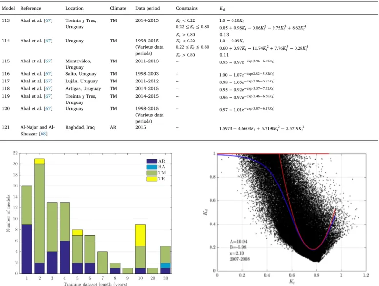
Fig. 1
presents the distribution of models as a function of the
number of years of the datasets and climate zone. Only the models that
presented an explicit dataset length in their respective publications
were used to produce
Fig. 1
. Models based on data from several
loca-tions, different climatic zones or models derived from distinct dataset
lengths were not considered, hence the 100 models examined in
Fig. 1
.
The higher number of models was developed for the temperate (TM)
zone, followed by the arid (AR), tropical (TR) and
finally the high
al-bedo (HA) zones. This representativeness of the climate zones is also
useful to perceive the distribution of solar radiation measuring stations
around the globe and how this may affect the model development. One
can conclude that the high albedo and the tropical climate zones are not
well represented. However, nowadays there are more meteorological
stations in these climate zones (see, e.g. Ref. [
69
]). The most typical
length of the training datasets is two years, followed by one, three and
four years. It worths to note that some authors used twenty and even
thirty years of data to derive their models (e.g. Refs. [
27
,
61
]).
3. Model development and test data
3.1. Model formulation
The model proposed in this study is based on the correlation of two
limiting functions for large and small values of
K
tthrough the
expres-sion disclosed by Churchill and Usagi [
70
] for the correlation of transfer
phenomena, described as follows:
=
+
Y
(1
Z
n n)
1(1)
where the arbitrary exponent n needs to be selected in order to correlate
those functions accurately [
70
]. This expression can be used to any
phenomenon varying uniformly, for example in heat transfer modelling
Table 1
Review of hourly and sub-hourly Kdmodels whose only predictor is Kt.
Model Reference Location Climate Data period Constrains Kd
1 Orgill and Hollands [15] Toronto, Canada TM 1967–1971 Kt≤0.35 1.0−0.249Kt ≤K ≤ 0.35 t 0.75 1.557−1.840Kt > Kt 0.75 0.177 2 Bruno [18] Hamburg, Germany TM 1973–1974 – 0.310Kt+0.139sin(4.620Kt) 3 Erbs et al. [19] Four cities in the
United States Various climates 1974–1976 (Various data periods) ≤ Kt 0.22 1.0−0.0900Kt <K ≤ 0.22 t 0.80 0.9511−0.1604Kt+4.3880Kt2−16.6380Kt3+12.3360Kt4 > Kt 0.80 0.165 4 Spencer [28] Albany, Australia AR 1973–1977 Kt<0.35 0.890
≤K ≤
0.35 t 0.75 1.414−1.736Kt
>
Kt 0.75 0.110 5 Spencer [28] Alice Springs,
Australia AR 1974–1977 Kt<0.35 0.750 ≤K ≤ 0.35 t 0.75 1.183−1.444Kt > Kt 0.75 0.110 6 Spencer [28] Geraldton, Australia AR 1972–1977 Kt<0.35 0.850 ≤K ≤ 0.35 t 0.75 1.345−1.644Kt > Kt 0.75 0.110 7 Spencer [28] Guildford, Australia AR 1975–1977 Kt<0.35 0.780 ≤K ≤ 0.35 t 0.75 1.254−1.595Kt > Kt 0.75 0.060 8 Spencer [28] Hobart, Australia TM 1971–1977 Kt<0.35 0.860
≤K ≤ 0.35 t 0.75 1.360−1.678Kt > Kt 0.75 0.100 9 Spencer [28] Laverton, Australia AR 1976–1977 Kt<0.35 0.860 ≤K ≤ 0.35 t 0.75 1.360−1.678Kt > Kt 0.75 0.150 10 Spencer [28] Melbourne, Australia AR 1970–1977 Kt<0.35 0.850 ≤K ≤ 0.35 t 0.75 1.352−1.668Kt > Kt 0.75 0.100 11 Spencer [28] Mildura, Australia AR 1972–1977 Kt<0.35 0.870
≤K ≤ 0.35 t 0.75 1.366−1.666Kt > Kt 0.75 0.120 12 Spencer [28] Mt Gambier, Australia AR 1974–1977 Kt<0.35 0.930 ≤K ≤ 0.35 t 0.75 1.450−1.744Kt > Kt 0.75 0.140 13 Spencer [28] Port Hedland,
Australia AR 1974–1977 Kt<0.35 0.710 ≤K ≤ 0.35 t 0.75 1.142−1.431Kt > Kt 0.75 0.070 14 Spencer [28] Rockhampton, Australia AR 1974–1977 Kt<0.35 0.790 ≤K ≤ 0.35 t 0.75 1.245−1.527Kt > Kt 0.75 0.100 15 Spencer [28] Waga Waga,
Australia AR 1974–1977 Kt<0.35 0.800 ≤K ≤ 0.35 t 0.75 1.280−1.605Kt > Kt 0.75 0.080 16 Spencer [28] Australia (average) Various climates 1970–1977 (Various data periods) < Kt 0.35 0.830 ≤K ≤ 0.35 t 0.75 1.321−1.624Kt > Kt 0.75 0.100 17 Hawlader [20] Singapore TM 1962 Kt<0.225 0.9150 ≤K ≤ 0.225 t 0.775 1.1389−0.9422Kt−0.3878Kt2 > Kt 0.775 0.2150 18 Ineichen et al. [29] Geneva,
Switzerland
TM 1978–1984 Kt<0.15 0.98 ≥
Kt 0.15 0.80+2.25Kt−7.93Kt2+5.26Kt3
19 Ineichen et al. [29] Geneva, Switzerland TM 1978–1984 Kt<0.25 1.0 ≤K ≤ 0.25 t 0.80 1.38−1.52Kt > Kt 0.80 0.16 20 Ineichen et al. [29] Geneva,
Switzerland
TM 1978–1984 Kt<0.25 1.0 ≥
Kt 0.25 1.28Kt−1.40Kt2
21 Muneer et al. [21] New Delhi, India TR 1971, 1974 Kt<0.175 0.9500 ≤K ≤
0.175 t 0.775 0.9698+0.4353Kt−3.4499Kt2+2.1888Kt3
>
Kt 0.775 0.2600 22 Bakhsh et al. [30] Dharan, Saudi
Arabia AR 1983–1984 Kt<0.23 1.0−0.220Kt ≤K ≤ 0.23 t 0.80 1.235−1.260Kt > Kt 0.80 0.225
23 Hollands [31] Toronto, Canada TM 1967–1971 – [1−b− (1−b)2−4ab K2 t(1−aKt) ]/(2abKt) =
a 1.115;b=0.491 24 Reindl et al. [6] Five locations in
North America and Europe Various climates 1979–1982 (Various data periods) ≤ Kt 0.30 1.020−0.248Kt <K < 0.30 t 0.78 1.450−1.670Kt ≥ Kt 0.78 0.147 25 Al-Rihai [32] Fudhaliyah, Iraq AR 1984–1987 Kt<0.25 0.932
≤K ≤
0.25 t 0.70 1.293−1.631Kt
>
Kt 0.70 0.151
Table 1 (continued)
Model Reference Location Climate Data period Constrains Kd
26 Bourges [33] 37 stations across Europe TM At least four years of measurements ≤ Kt 0.20 1.0 <K ≤ 0.20 t 0.35 1.116−0.580Kt <K ≤ 0.35 t 0.75 1.557−1.840Kt > Kt 0.75 0.177 27 Chandrasekaran and Kumar [34] Madras, India TR 1983–1987 Kt≤0.24 1.0086−0.1780Kt <K ≤ 0.24 t 0.80 0.9686+0.1325Kt+1.4183Kt2−10.1860Kt3+8.3733Kt4 > Kt 0.80 0.1970 28 Chendo and Maduekwe [35]
Lagos, Nigeria TM Two years of measurements ≤ Kt 0.30 1.022−0.156Kt <K < 0.30 t 0.80 1.385−1.396Kt ≥ Kt 0.80 0.264 29 Maduekwe and Chendo [36] Lagos, Nigeria TM 1990–1991 Kt≤0.30 1.021−0.151Kt <K < 0.30 t 0.80 1.385−1.396Kt ≥ Kt 0.80 0.295 30 Lam and Li [37] Hong Kong, China TM 1991–1994 Kt≤0.15 0.977
<K ≤
0.15 t 0.70 1.237−1.361Kt
>
Kt 0.70 0.273 31 Hijazin [38] Amman, Jordan AR 1985 Kt<0.10 0.744
≤K ≤
0.10 t 0.80 0.842−0.977Kt
>
Kt 0.80 0.060 32 Hijazin [38] Amman, Jordan AR 1985 – 0.847−0.985Kt
33 González and Calbó [39] Two locations in Iberian Peninsula TM 1994–1996 (Various data periods) <K < 0.25 t 0.75 1.421−1.670Kt ≥ Kt 0.75 −0.043+0.290Kt
34 Boland et al. [26] Geelong, Australia TM 67 days – 1.0/[1.0+exp{8.645(Kt−0.613)}] 35 Boland et al. [26] Geelong, Australia TM 67 days – 1.0/[1.0+exp{7.997(Kt−0.586)}] 36 De Miguel et al. [40] North Mediterranean belt area (11 stations) TM 1974–1996 (Various data periods) ≤ Kt 0.21 0.995−0.081Kt <K ≤ 0.21 t 0.76 0.724+2.738Kt−8.320Kt2+4.967Kt3 > Kt 0.76 0.180 37 Li and Lam [41] Hong Kong, China TM 1991–1998 Kt≤0.15 0.976
<K ≤
0.15 t 0.70 0.996+0.036Kt−1.589Kt2
>
Kt 0.70 0.230
38 Oliveira et al. [42] São Paulo, Brazil TM 1994–1999 0.17<Kt<0.75 0.97+0.80Kt−3.00Kt2−3.1Kt3+5.2Kt4
39 Ulgen and Hepbasli [43] Izmir, Turkey TM 1994–1998 Kt≤0.32 0.6800 <K ≤ 0.32 t 0.62 1.0609−1.2138Kt > Kt 0.62 0.3000 40 Ulgen and Hepbasli [43] Izmir, Turkey TM 1994–1998 Kt≤0.32 0.6800 <K ≤ 0.32 t 0.62 0.0743−19.3430Kt+206.9100Kt2−719.7200Kt3+1053.4000Kt4−562.69Kt5 > Kt 0.62 0.3000 41 Karatasou et al. [44] Athens, Greece TM 1996–1998 Kt≤0.78 0.9995−0.0500Kt−2.4156Kt2+1.4926Kt3 > Kt 0.78 0.2000 42 Tsubo and Walker
[45]
Southern Africa AR 2000 – 0.613−0.334Kt+0.121Kt2
43 Tsubo and Walker [45] Southern Africa AR 2000 Kt<0.140 0.907 ≤K ≤ 0.140 t 0.794 > Kt 0.794 0.138 44 Tsubo and Walker
[45] Southern Africa AR 2000 Kt<0.140 0.907 ≤K ≤ 0.140 t 0.794 1.063−1.114Kt > Kt 0.793 0.180
45 Soares et al. [46] São Paulo, Brazil TM 1998–2001 – 0.90+1.10Kt−4.50Kt2+0.01Kt3+3.14Kt4
46 Mondol et al. [47] Ballymena, Northern Ireland TM 21 months of data ≤ Kt 0.20 0.9800 > Kt 0.20 0.5836+3.6259Kt−10.1710Kt2+6.3380Kt3 47 Jacovides et al. [48] Athalassa, Cyprus AR 1998–2002 Kt≤0.10 0.987 <K ≤ 0.10 t 0.80 0.940+0.937Kt−5.010Kt2+3.320Kt3 > Kt 0.80 0.177 48 Elminir et al. [49] Aswan, Egypt AR 1999–2001 Kt≤0.22 0.653−1.728Kt
<K ≤
0.22 t 0.80 0.724−1.821Kt+8.221Kt2−16.370Kt3+9.845Kt4
>
Kt 0.80 0.217 49 Elminir et al. [49] Cairo, Egypt AR 2003 Kt≤0.22 0.793−2.198Kt
<K ≤
0.22 t 0.80 1.341−9.566Kt+32.200Kt2−47.909Kt3+25.419Kt4
>
Kt 0.80 0.131 50 Elminir et al. [49] South-Valley,
Egypt AR 2003 Kt≤0.22 0.8526−1.7780Kt <K ≤ 0.22 t 0.80 0.8140−1.1060Kt+0.3660Kt2−0.9970Kt3+1.2210Kt4 > Kt 0.80 0.213 51 Boland et al. [50] Adelaide,
Australia
AR – – 1.0/[1.0+exp( 5.83− +9.87Kt)] 52 Boland et al. [50] Bracknell,
England
TM – – 1.0/[1.0+exp( 4.38− +6.62Kt)] 53 Boland et al. [50] Darwin, Australia TM – – 1.0/[1.0+exp( 4.53− +8.05Kt)] 54 Boland et al. [50] Lisbon, Portugal TM – – 1.0/[1.0+exp( 4.80− +7.98Kt)] 55 Boland et al. [50] Macau, China TM – – 1.0/[1.0+exp( 4.87− +8.12Kt)]
Table 1 (continued)
Model Reference Location Climate Data period Constrains Kd
56 Boland et al. [50] Maputo, Mozambique
AR – – 1.0/[1.0+exp( 5.18− +8.80Kt)] 57 Boland et al. [50] Uccle, Belgium TM – – 1.0/[1.0+exp( 4.94− +8.66Kt)] 58 Boland et al. [50] Multi-location
average
Various climates
– – 1.0/[1.0+exp( 4.94− +8.30Kt)]
59 Boland and Ridley [51] Multi-locations worldwide Various climates – – 1.0/[1.0+exp( 5.00− +8.60Kt)] 60 Furlan and Oliveira [52]
Sâo Paulo, Brazil TM 2002 Kt≤0.228 0.961 >
Kt 0.228 1.337−1.650Kt
61 Mondol et al. [53] Aldergrove, Northern Irland TM 1989–1998 Kt≤0.20 0.9800 <K ≤ 0.20 t 0.70 0.6109+3.6259Kt−10.1710Kt2+6.3380Kt3 > Kt 0.70 0.6720−0.4740Kt
62 Moreno et al. [54] Seville, Spain TM 2000–2008 Kt≤0.27 0.9930 <K ≤
0.27 t 0.82 1.4946−1.7899Kt
>
Kt 0.82 0.0450 63 Pagola et al. [55] 3 locations in
Spain TM 2005–2008 Kt≤0.35 0.9818−0.5870Kt <K ≤ 0.35 t 0.75 1.2056−1.3240Kt > Kt 0.75 0.2552 64 Pagola et al. [55] 3 locations in
Spain TM 2005–2008 Kt≤0.22 0.9522−0.3119Kt <K ≤ 0.22 t 0.80 0.6059+2.9877Kt−10.5675Kt2+10.1833Kt3−3.0475Kt4 > Kt 0.80 0.3209 65 Posadillo and Lopez Luque [56] Córdoba, Spain TM 1993–2002 – Kt(1.17−1.381Kt) 66 Posadillo and Lopez Luque [56] Córdoba, Spain TM 1993–2002 – −0.00829+1.16300Kt+0.43300Kt2−5.83900Kt3+4.64880Kt4
67 Janjai et al. [57] Chiang Mai, Thailand
TR 1995–2006 – 0.9429−0.3707Kt+6.4927Kt2−30.3560Kt3+39.1626Kt4−15.4850Kt5
68 Janjai et al. [57] Nakhon Pathom, Thailand
TR 1995–2006 – 0.7699+2.3552Kt−8.1480Kt2+5.3811Kt3
69 Janjai et al. [57] Songkhla, Thailand
TR 1995–2006 – 0.869+1.559Kt−11.176Kt2+26.143Kt3−38.302Kt4+31.799Kt5−10.602Kt6
70 Janjai et al. [57] Ubon Ratchathani, Thailand
TR 1995–2006 – 0.846+1.841Kt−13.425Kt2+42.888Kt3−85.804Kt4+84.476Kt5−30.637Kt6
71 Ruiz-Arias et al. [27]
Albacete, Spain TM 2002–2006 – 0.086+0.880e−exp( 3.877 6.138− + Kt) 72 Ruiz-Arias et al.
[27]
Boulder, USA TM 1961–1990 – 0.967−1.024e−exp(2.473 5.324− Kt) 73 Ruiz-Arias et al.
[27]
Dresden, Germany TM 1981–1990 – 0.140+0.962e−exp( 1.976 4.067− + Kt) 74 Ruiz-Arias et al.
[27]
Pittsburgh, USA TM 1961–1990 – 1.001−1.000e−exp(2.450 5.048− Kt) 75 Ruiz-Arias et al.
[27]
Savannah, USA TM 1961–1990 – 0.988−1.000e−exp(2.456 5.172− Kt) 76 Ruiz-Arias et al.
[27]
Talkeetna, USA HA 1961–1990 – 0.985−0.962e−exp(2.655 6.003− Kt) 77 Ruiz-Arias et al.
[27]
Tucson, USA AR 1961–1990 – 0.988−1.073e−exp(2.298 4.909− Kt) 78 Ruiz-Arias et al.
[27]
7 locations in Europe and USA
Various climates 1961–2006 (Various data periods) – 0.952−1.041e−exp(2.3 4.702− Kt)
79 Torres et al. [58] Pamplona, Spain TM 2006–2008 Kt≤0.24 1.0058−0.2195Kt
<K <
0.24 t 0.75 1.3264−1.5120Kt
≥
Kt 0.75 0.1923 80 Torres et al. [58] Pamplona, Spain TM 2006–2008 Kt≤0.22 0.9920−0.0980Kt
<K <
0.22 t 0.75 1.2158−1.0467Kt−0.4480Kt2
≥
Kt 0.75 0.1787 81 Torres et al. [58] Pamplona, Spain TM 2006–2008 Kt≤0.22 0.9923−0.0980Kt
<K ≤
0.24 t 0.755 1.1459−0.5612Kt−1.4952Kt2+0.7103Kt3
>
Kt 0.755 0.1755 82 Torres et al. [58] Pamplona, Spain TM 2006–2008 Kt≤0.225 0.9943−0.1165Kt
<K ≤
0.225 t 0.755 1.4101−2.9918Kt+6.4599Kt2−10.3290Kt3+5.5140Kt4
>
Kt 0.755 0.1800 83 Chikh et al. [59] Alger, Algeria AR 1992 Kt≤0.175 1.0−0.232Kt
<K ≤
0.175 t 0.87 1.170−1.230Kt
>
Kt 0.87 0.203 84 Chikh et al. [59] Bechar, Algeria AR 1990–1992 Kt≤0.175 1.0−0.3000Kt
<K ≤
0.175 t 0.87 1.1370−1.0770Kt
>
Kt 0.87 0.2043 85 Chikh et al. [59] Tamanrasset,
Algeria AR 1990–1992 Kt≤0.175 1.0−0.640Kt <K ≤ 0.175 t 0.87 1.052−0.935Kt > Kt 0.87 0.240 86 Sanchez et al. [60] Badajoz, Spain TM 2009–2010 Kt<0.30 0.78
≤K ≤
0.30 t 0.75 1.23−1.43Kt
>
Kt 0.75 0.13
Table 1 (continued)
Model Reference Location Climate Data period Constrains Kd
87 Lee et al. [61] South Korea TM 1986–2005 Kt≤0.20 0.9200 >
Kt 0.20 0.6910+2.4306Kt−7.3371Kt2+4.7002Kt3
88 Yao et al. [62] Shanghai, China TM 2012 Kt≤0.30 0.9381−0.1481Kt
<K ≤
0.30 t 0.80 1.5197−1.5340Kt
>
Kt 0.80 0.2700
89 Yao et al. [62] Shanghai, China TM 2012 – 0.8142+2.0792Kt−6.1439Kt2+3.4707Kt3
90 Yao et al. [62] Shanghai, China TM 2012 Kt≤0.20 0.8755+1.3991Kt−4.9285Kt2
<K ≤
0.20 t 0.80 1.1209−2.1699Kt+11.0600Kt2−22.3550Kt3+12.8630Kt4
>
Kt 0.80 0.2700
91 Yao et al. [62] Shanghai, China TM 2012 – 0.2421+0.7202/[1+exp{(Kt−0.6203)/0.0749}] 92 Tapakis et al. [63] Athalassa, Cyprus AR 2001–2010 Kt<0.10 0.9100+2.4993Kt−18.8580Kt2
≤K ≤
0.10 t 0.78 0.9605+0.4482Kt−2.0011Kt2−1.5581Kt3+2.0080Kt4
>
Kt 0.78 −2.4518+3.3014Kt
93 Abreu et al. [64] Évora, Portugal TM 2015–2016 – [1.0+(1.502−1.820K)− ]−
t 48.589 1.0/48.589 94 Marques Filho et al. [65] Rio de Janeiro, Brazil TM 2011–2014 – 1.0/[1.0+exp( 4.90− +8.78Kt)] 95 Marques Filho et al. [65] Rio de Janeiro, Brazil TM 2011–2014 – 0.13+0.86/[1.0+exp( 6.29− +12.26Kt)] 96 Paulescu and Blaga [66] Timisoara, Romania TM 2009–2010 Kt<0.247 0.936+0.194Kt ≥ Kt 0.247 1.436−1.824Kt
97 Abal et al. [67] Montevideo, Uruguay TM 2011–2013 Kt<0.20 1.0 ≤K ≤ 0.20 t 0.85 0.50+5.92Kt−22.22Kt2+29.51Kt3−19.54Kt4+6.09Kt5 > Kt 0.85 0.10 98 Abal et al. [67] Salto, Uruguay TM 1998–2003 Kt<0.20 1.0
≤K ≤
0.20 t 0.85 0.72+2.80Kt−6.62Kt2−4.66Kt3+14.13Kt4−6.20Kt5
>
Kt 0.85 0.09 99 Abal et al. [67] Luján, Uruguay TM 2011–2012 Kt<0.20 1.0
≤K ≤
0.20 t 0.85 0.80+1.97Kt−3.93Kt2−5.97Kt3+10.96Kt4−3.56Kt5
>
Kt 0.85 0.11 100 Abal et al. [67] Artigas, Uruguay TM 2014–2015 Kt<0.20 1.0
≤K ≤
0.20 t 0.85 0.86+0.87Kt+3.53Kt2−28.43Kt3+39.51Kt4−16.21Kt5
>
Kt 0.85 0.11 101 Abal et al. [67] Treinta y Tres,
Uruguay TM 2014–2015 Kt<0.20 1.0 ≤K ≤ 0.20 t 0.85 1.04−1.45Kt+13.21Kt2−43.80Kt3+48.79Kt4−17.60Kt5 > Kt 0.85 0.12 102 Abal et al. [67] Uruguay TM 1998–2015
(Various data periods) < Kt 0.20 1.0 ≤K ≤ 0.20 t 0.85 0.77+2.16Kt−3.91Kt2−9.02Kt3+17.00Kt4−6.79Kt5 > Kt 0.85 0.10 103 Abal et al. [67] Montevideo,
Uruguay TM 2011–2013 Kt<0.35 1.0−0.40Kt ≤K ≤ 0.35 t 0.75 1.51−1.86Kt > Kt 0.75 0.12 104 Abal et al. [67] Salto, Uruguay TM 1998–2003 Kt<0.35 1.0−0.29Kt
≤K ≤
0.35 t 0.75 1.60−2.00Kt
>
Kt 0.75 0.10 105 Abal et al. [67] Luján, Uruguay TM 2011–2012 Kt<0.35 1.0−0.24Kt
≤K ≤
0.35 t 0.75 1.60−1.95Kt
>
Kt 0.75 0.14 106 Abal et al. [67] Artigas, Uruguay TM 2014–2015 Kt<0.35 1.0−0.33Kt
≤K ≤
0.35 t 0.75 1.56−1.93Kt
>
Kt 0.75 0.11 107 Abal et al. [67] Treinta y Tres,
Uruguay TM 2014–2015 Kt<0.35 1.0−0.19Kt ≤K ≤ 0.35 t 0.75 1.63−1.99Kt > Kt 0.75 0.14 108 Abal et al. [67] Uruguay TM 1998–2015
(Various data periods) < Kt 0.35 1.0−0.28Kt ≤K ≤ 0.35 t 0.75 1.59−1.96Kt > Kt 0.75 0.12 109 Abal et al. [67] Montevideo,
Uruguay TM 2011–2013 Kt<0.22 1.0−0.24Kt ≤K ≤ 0.22 t 0.80 0.70+2.63Kt−7.38Kt2+1.86Kt3+2.67Kt4 > Kt 0.80 0.13 110 Abal et al. [67] Salto, Uruguay TM 1998–2003 Kt<0.22 1.0
≤K ≤
0.22 t 0.80 0.38+6.54Kt−21.25Kt2+21.37Kt3−6.99Kt4
>
Kt 0.80 0.09 111 Abal et al. [67] Luján, Uruguay TM 2011–2012 Kt<0.22 1.0−0.06Kt
≤K ≤
0.22 t 0.80 0.62+3.70Kt−10.83Kt2+7.00Kt3−0.30Kt4
>
Kt 0.80 0.12 112 Abal et al. [67] Artigas, Uruguay TM 2014–2015 Kt<0.22 1.0−0.15Kt
≤K ≤
0.22 t 0.80 0.68+2.91Kt−7.75Kt2+1.47Kt3+3.24Kt4
>
Kt 0.80 0.13
[
71
] and
fluid flow and heat transfer optimisation when combined with
the concept of the intersection of asymptotes [
72
,
73
]. In the case of
modelling the diffuse fraction as a function of the clearness index, the
functions used here are the physically possible limit of
K
d=
1
and a
function Z that is the best
fit for the clear sky periods. The occurrence of
cloud enhancement effects in 1-min resolution data is quite frequent
[
1
,
14
], then function Z was defined as the best fit to the clear sky data
using a second degree polynomial in the form:
=
−
+
−
+
Z
A K
(
t0.5)
2B K
(
t0.5)
1
(2)
Since
K
dis a concave function of
K
t, the exponents used in Eq.
(1)
must be − n and −
1/ , and thus, the
n
final form of the model is given
by:
=
+
−
+
−
+
− −K
d{1
[ (
A K
t0.5)
2B K
(
t0.5)
1] }
n n1
(3)
Fig. 2
shows the
fitting of the model to the data of Fort Peck station
(FPE), USA, as an example of the procedures implemented in this work
for all the analysed stations. Red lines represent the limiting functions
=
K
d1
and Z (
fitted to the FPE dataset), and the blue line represents the
fitted model. The three parameters of the adjusted model for FPE
sta-tion are also presented, as well as the period of data used.
3.2. Test stations and data quality control
The data used in this study is from the Baseline Surface Radiation
Network (BSRN) [
69
,
74
] and the Institute of Earth Sciences (IES) at the
University of Évora, Portugal. The BSRN is a project of the Global
En-ergy and Water Cycle Experiment (GEWEX) under the umbrella of the
World Climate Research Programme (WCRP). The primary objective of
this network is to detect changes in the radiation
field at the Earth's
surface which may be related to climate changes. Measurements of
solar radiation in the IES station are taken likewise as in the BSRN
stations: the di
ffuse horizontal irradiation (DHI) is measured by a Kipp&
Zonnen CM6B pyranometer and shading ball attached to the sun tracker
and the global horizontal irradiance is also measured by a Kipp&
Zonnen CM6B pyranometer. The sensors are installed on a Kipp&
Zonnen Solys2 sun tracker and are properly maintained and calibrated
according to the BSRN and WMO guidelines and recommendations
[
69
,
75
].
Table 2
shows detailed information on the stations used in this
study: location, climate zone, data period, number of valid data points
and mean GHI of all valid measurements.
Data quality control was performed by applying the quality
filters
de
fined by Long and Shi [
76
] for the global horizontal irradiance (GHI).
Furthermore,
K
dvalues higher than 1 and lower than 0 were removed
Table 1 (continued)Model Reference Location Climate Data period Constrains Kd
113 Abal et al. [67] Treinta y Tres, Uruguay TM 2014–2015 Kt<0.22 1.0−0.10Kt ≤K ≤ 0.22 t 0.80 0.85+0.98Kt−0.06Kt2−9.75Kt3+8.62Kt4 > Kt 0.80 0.13 114 Abal et al. [67] Uruguay TM 1998–2015
(Various data periods) < Kt 0.22 1.0−0.09Kt ≤K ≤ 0.22 t 0.80 0.60+3.97Kt−11.74Kt2+7.76Kt3−0.28Kt4 > Kt 0.80 0.11 115 Abal et al. [67] Montevideo,
Uruguay
TM 2011–2013 – 0.95−0.97e−exp(2.96 6.07− Kt) 116 Abal et al. [67] Salto, Uruguay TM 1998–2003 – 1.00−1.07e−exp(2.82 5.82− Kt) 117 Abal et al. [67] Luján, Uruguay TM 2011–2012 – 0.98−1.05e−exp(2.96 5.75− Kt) 118 Abal et al. [67] Artigas, Uruguay TM 2014–2015 – 0.95−0.92e−exp(3.57 7.32− Kt) 119 Abal et al. [67] Treinta y Tres,
Uruguay
TM 2014–2015 – 0.96−0.97e−exp(3.46 6.68− Kt) 120 Abal et al. [67] Uruguay TM 1998–2015
(Various data periods)
– 0.97−1.01e−exp(3.07 6.17− Kt)
121 Najar and Al-Khazzar [68]
Baghdad, Iraq AR 2015 – 1.5973−4.6603Kt+5.7190Kt2−2.5719Kt3
Fig. 1. Distribution of the models according to the length of the training da-tasets and climate zone: temperate (TM), arid (AR), tropical (TR) and high al-bedo (HA).
Fig. 2. Data for the FPE station (Fort Peck, USA) and representation of the limiting functions (red) and model correlation (blue). (For interpretation of the
references to colour in thisfigure legend, the reader is referred to the Web
for the
fitting of the model parameters A and B, since measurements of
di
ffuse irradiance higher than global irradiance are very dubious.
However, instrumental errors can occur, and therefore, the
K
dmax-imum value was set to 1.2 when determining the parameter n. Finally,
measurements taken when the zenith angle was higher than
85
∘were
also removed due to disturbances caused mainly by the horizon line and
also due to instrumental and modelling accuracy issues in that case
[
14
]. Since 1-min data was used in this work, the extraterrestrial
irra-diance on a horizontal surface,
E
oh, that is needed to determine the
K
twas simply calculated based on the solar constant (
G
=
1361.1
Wm
−s 2
[
77
]) and the solar zenith angle, this last being calculated through the
very accurate solar position algorithm developed by Reda and Andreas
[
78
]. The data was divided into two sets: the training set with two years
of data used to determine the
fitting parameters of the proposed model;
and the validation set with one year of data, used to validate the
de-veloped model as well as the models available in the literature (Section
2
). These datasets are composed of years with high number of valid
measurements, i.e., records that successfully passed the quality control
procedures [
76
], as shown in
Table 2
.
3.3. Statistical indicators for model assessment
The developed model, as well as the models reviewed in Section
2
,
were evaluated using the statistical indicators described below taking
the measured values as reference. Lower values indicate better model
accuracy except for the mean bias error and mean percentage error, in
which values closer to zero indicate a better model accuracy, and for
the correlation coefficient, in which a value closer to 1 represents better
model accuracy. In the following, H and N stand for minutely di
ffuse
horizontal irradiance (DHI) and number of observations, respectively,
and the subscripts m, e and
avg
stand for measured, estimated and
average, respectively.
3.3.1. Mean bias error (MBE)
∑
=
−
=N
H
H
MBE
1
(
)
i N e i m i 1 , ,(4)
Table 2Information on the data of BSRN and IES stations. Acronyms: AR (Arid), HA (High albedo), TM (Temperate), and TR (Tropical).
Station Code Lat. (°N) Long. (°E) Elev. (m) Climate Data period Samples Mean GHI (W m/ 2)
Alert ALE 82.490 −62.420 127 HA 2009–2011 631284 223.84
Alice Springs ASP −23.798 133.888 547 AR 2007–2009 704784 561.96
Bermuda BER 32.267 −64.667 8 TM 2006–2008 458837 497.33 Billings BIL 36.605 −97.516 317 TM 2005–2007 631822 451.65 Bondville BON 40.067 −88.367 213 TM 2007–2009 220046 507.54 Boulder BOU 40.050 −105.007 1577 TM 2002–2004 481571 519.33 Brasilia BRB −15.601 −47.713 1023 TR 2009–2011 598116 472.22 Carpentras CAR 44.083 5.059 100 TM 2003–2005 619585 419.19 Chesapeake Light CLH 36.905 −75.713 37 TM 2011–2013 681269 408.60 Cener CNR 42.816 −1.601 471 TM 2010–2012 666202 374.60
Cocos Island COC −12.193 96.835 6 TR 2006–2008 556163 505.99
De Aar DAA −30.667 23.993 1287 AR 2002–2004 592787 518.07
Darwin DAR −12.425 130.891 30 TR 2009–2011 699416 489.94
Concordia station DOM −75.100 123.383 3233 HA 2005–2007 255370 377.86
Desert Rock DRA 36.626 −116.018 1007 AR 2007–2009 324644 596.47
Évora EVR 38.568 −7.912 293 TM 2016–2017 199169 504.11
Eureka EUR 79.989 −85.940 85 HA 2009–2011 654421 230.99
Fort Peck FPE 48.317 −105.100 634 TM 2007–2009 227621 481.02
Fukuoka FUA 33.582 130.376 3 TM 2011–2013 715368 337.10
Goodwin Creek GCR 34.250 −89.870 98 TM 2007–2009 244471 529.24
Gobabeb GOB −23.561 15.042 407 AR 2012–2014 627165 596.64
Georg von Neumayer GVN −70.650 −8.250 42 HA 2011–2013 509631 316.63
Ilorin ILO 8.533 4.567 350 TR 1995,1999,2000 160661 307.77 Ishigakijima ISH 24.337 124.163 6 TM 2011–2013 710421 374.30 Izana IZA 28.309 −16.499 2373 AR 2011–2013 680660 612.14 Kwajalein KWA 8.720 167.731 10 TR 1998–2000 517467 544.96 Lauder LAU −45.045 169.689 350 TM 2005–2007 583349 399.17 Lerwick LER 60.139 −1.185 80 TM 2004–2006 586958 213.18 Lindenberg LIN 52.210 14.122 125 TM 2001–2003 665675 285.77 Momote MAN −2.058 147.425 6 TR 2008–2010 689159 470.82 Minamitorishima MNM 24.288 153.983 7 TM 2011–2013 727974 470.67
Nauru Island NAU −0.521 166.917 7 TR 2005–2007 649304 513.96
Ny-Alesund NYA 78.925 11.930 11 HA 2007–2009 619576 187.06
Palaiseau PAL 48.713 2.208 156 TM 2009–2011 701389 302.24
Payerne PAY 46.815 6.944 491 TM 2008–2010 573646 349.50
Rock Springs PSU 40.720 −77.933 376 TM 2007–2009 203868 471.41
Petrolina PTR −9.068 −40.319 387 TR 2007–2009 149097 566.04
Regina REG 50.205 −104.713 578 TM 2009–2011 620001 365.50
Sapporo SAP 43.060 141.328 17 AR 2011–2013 722699 305.91
Sede Boqer SBO 30.860 34.779 480 TM 2009–2011 662564 542.45
Sonnblick SON 47.054 12.958 3109 HA 2013–2015 462080 371.23
Solar Village SOV 24.907 46.397 768 AR 2000–2002 717011 564.91
Sioux Falls SXF 43.730 −96.620 473 TM 2007–2009 228600 475.41 Tamanrasset TAM 22.790 5.529 1385 AR 2006–2008 644908 596.17 Tateno TAT 36.050 140.133 25 TM 2008–2010 683402 334.39 Tiksi TIK 71.586 128.919 48 HA 2011–2013 617716 211.72 Toravere TOR 58.254 26.462 70 TM 2010–2012 649189 245.32 Xianghe XIA 39.754 116.962 32 TM 2008–2010 561393 381.54
3.3.2. Mean absolute error (MAE)
∑
=
−
=N
H
H
MAE
1
|
|
i N e i m i 1 , ,(5)
3.3.3. Root mean square error (RMSE)
∑
=
⎡
⎣
⎢
−
⎤
⎦
⎥
=N
H
H
RMSE
1
(
)
i N e i m i 1 , , 2 1 2(6)
3.3.4. Mean percentage error (MPE)
∑
⎜ ⎟=
⎛
⎝
−
⎞
⎠
×
=N
H
H
H
MPE
1
100
i N e i m i m i 1 , , ,(7)
3.3.5. Uncertainty at 95% (U95)
=
SD
+
RMSE
U95
1.96(
2 2)
12(8)
where
SD
represents the standard deviation of the difference between
H
eand H
m.
3.3.6. Relative root mean square error (RRMSE)
=
RMSE
H
RRMSE
m avg,(9)
3.3.7. T-statistics (TSTAT)
=⎡
⎣
⎢
−
−
⎤
⎦
⎥
N
MBE
RMSE
MBE
TSTAT
(
1)
2 2 2 1 2(10)
3.3.8. Maximum absolute relative error (erMAX)
=
⎧
⎨
⎩
−
=
…
⎫
⎬
⎭
H
H
H
i
N
erMAX
max |
e i m i|,
1, ,
m i , , ,(11)
3.3.9. Correlation coefficient (R)
=
∑
−
−
∑
−
∑
−
= = =H
H
H
H
H
H
H
H
R
(
)(
)
(
)
(
)
i N e i e avg m i m avg i N e i e avg i N m i m avg 1 , , , , 1 , , 2 1 , , 2(12)
3.3.10. Mean absolute relative error (MARE)
∑
=
−
=N
H
H
H
MARE
1
|
|
i N e i m i m i 1 , , ,(13)
3.3.11. Global performance index (GPI)
The global performance index,
firstly proposed by Behar et al. [
79
],
then modified by Despotovic et al. [
80
] and used by Jamil and Akthar
[
23
,
81
], is also used here to combine all the statistical indicators
pre-sented in
Subsections 3.3.1 to 3.3.10
. The need for using this index is
due to the incapacity of those statistical indicators to, consistently,
identify the best model (see
Table 4
). The values of the statistical
in-dicators need to be scaled between 0 (worst performing model) and 1
(best performing model) to determine the GPI values, which otherwise
would make difficult to compare the models. This normalisation also
allows using the same statistical weight for all of the indicators when
determining the GPI, as follows:
∑
=
−
=α y
y
GPI
( ¯
)
j j j ij 1 10(14)
where
y
¯
jis the median of the scaled values of the indicator j,
y
ijis the
scaled value of the statistical indicator j for the model i, and
α
jequals to
1 for all statistical indicators except R, in which
α
jequals to
−1. The
GPI also allows to combine several indicators regardless if the value of a
single indicator is 0 or not, which is not possible if a simple product of
Fig. 3. Relative frequency of Ktin BSRN stations
the indicators is computed, and therefore a higher GPI stands for better
accuracy of a given model.
4. Results and discussion
4.1. Determination of model parameters and climate analysis
Fig. 3
shows the distribution of the
K
tvalues for the climate zones
considered, which is useful to identify the range of the clearness index
and the clear sky occurrences (frequency). The AR climate zone
pre-sents the highest relative frequency for high values of
K
t, reaching a
relative frequency of 0.038 for
K
t≃
0.77
, followed by the TM and TR
climate zones with maximum relative frequency around 0.030 for
ap-proximately the same
K
tvalue. The HA climate zone presents the lower
values of
K
trelative frequency for clear sky.
The training of the model was performed using the stations from the
BSRN network, while the IES station (EVR) was used only in the
vali-dation of the model. The parameters A and B for each station were
found by
fitting Eq.
(2)
to the data in the range of
K
t≥
0.5
, using the
non-linear least squares method. Then, the parameter n was obtained
through an optimisation process in order to achieve the maximum GPI
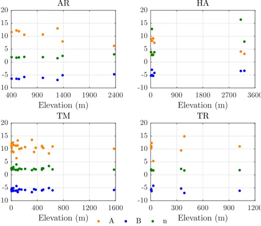
value for the entire range of the data. One also investigated the
ex-istence of a possible relationship between these parameters and the
elevation of the stations according to the climate zone, as shown in
Fig. 4
. However no conclusions can be drawn on the existence of any
clear dependence, and therefore, no traditional
fitting equations using
the parameters of the model and the elevation of the stations were able
to present an acceptable coefficient of determination.
To develop a model based only on the
K
tas predictor for each
cli-mate region, the mean value and standard deviation of these
para-meters were calculated for the four zones considered, and the stations
in which at least one of the three parameters were out of the confidence
interval de
fined by the mean
±
standard deviation were excluded from
this calculation. After this procedure, the values inside this imposed
range are averaged in order to obtain the mean values of A, B and n for
each climate zone, as shown in
Table 3
. These parameters were used for
the model performance assessment as presented in the following
sec-tion.
4.2. Performance assessment
The statistical tools presented in Section
3.3
were used to assess the
performance of the models from the literature as well as of the model
developed in this work using measurements from the EVR station and
the datasets from the BSRN, as presented in
Table 2
. The performance
assessment was carried out using the corresponding set of parameters
according to the climate zone of the 48 radiometric stations analysed in
this study. The performance assessment is presented in detail for the
EVR station as an example of both the methodology used in this study
and as a completely independent assessment since data from this station
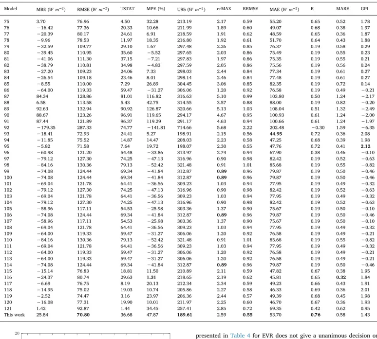
was not included in the determination of the model parameters.
Table 4
presents the results of the statistical analysis of the selected models
using the indicators shown in Section
3.3
for the EVR station. The bold
font indicates the optimal values of the statistical indicators, i.e., it
indicates the best model according to each statistical indicator.
The statistical evaluation regarding the accuracy of the models
Fig. 4. Variation of the parameters A, B and n according to the elevation of the stations and climate zone: Arid (AR), High Albedo (HA), Temperate (TM) and Tropical (TR).
Table 3
Parameters of the developed model according to the climate zone: Arid (AR), High Albedo (HA), Temperate (TM) and Tropical (TR).
Parameters Climate Zone
AR HA TM TR
A 11.39 7.83 10.79 11.59
B −6.25 −4.59 −5.87 −6.14
Table 4
Statistical analysis of the selected models for the EVR station.
Model MBE (W m−2) RMSE (W m−2) TSTAT MPE (%) U95 (W m−2) erMAX RRMSE MAE (W m−2) R MARE GPI
1 −40.31 111.13 36.42 −6.42 297.74 2.00 0.86 75.41 0.19 0.55 0.22 2 −29.87 102.79 28.42 3.82 278.84 2.11 0.79 71.26 0.30 0.54 0.64 3 −46.36 112.67 42.25 −12.76 298.80 1.79 0.87 75.05 0.19 0.53 0.13 4 −74.08 124.44 69.34 −41.84 312.87 0.89 0.96 79.87 0.19 0.50 −0.46 5 −79.12 127.30 74.25 −47.13 316.96 0.90 0.98 82.42 0.19 0.52 −0.63 6 −74.08 124.44 69.34 −41.84 312.87 0.89 0.96 79.87 0.19 0.50 −0.46 7 −99.29 140.53 93.43 −68.28 337.45 0.94 1.08 99.29 0.19 0.68 −1.46 8 −79.12 127.30 74.25 −47.13 316.96 0.90 0.98 82.42 0.19 0.52 −0.63 9 −53.92 115.14 49.60 −20.69 301.16 1.54 0.89 75.16 0.19 0.51 0.00 10 −79.12 127.30 74.25 −47.13 316.96 0.90 0.98 82.42 0.19 0.52 −0.63 11 −69.04 121.78 64.41 −36.56 309.23 1.03 0.94 77.95 0.19 0.49 −0.32 12 −58.96 117.11 54.53 −25.98 303.36 1.37 0.90 75.67 0.19 0.50 −0.10 13 −94.25 136.99 88.73 −62.99 331.75 0.93 1.06 94.31 0.19 0.63 −1.24 14 −79.12 127.30 74.25 −47.13 316.96 0.90 0.98 82.42 0.19 0.52 −0.63 15 −89.21 133.59 83.95 −57.70 326.42 0.92 1.03 89.69 0.19 0.58 −1.02 16 −79.12 127.30 74.25 −47.13 316.96 0.90 0.98 82.42 0.19 0.52 −0.63 17 −21.15 109.03 18.51 13.67 299.35 2.64 0.84 78.71 0.19 0.64 0.24 18 28.34 79.71 35.61 56.30 213.84 2.98 0.62 63.06 0.68 0.69 0.91 19 −48.88 113.43 44.69 −15.41 299.45 1.71 0.88 75.01 0.19 0.52 0.09 20 −38.25 107.47 35.65 −3.12 288.30 2.10 0.83 69.93 0.24 0.49 0.45 21 1.53 112.10 1.28 37.46 310.72 3.40 0.87 85.97 0.19 0.78 −0.01 22 −16.11 109.19 13.96 18.96 301.01 2.81 0.84 80.05 0.19 0.67 0.20 23 0.42 82.32 0.48 28.96 228.18 2.45 0.64 54.46 0.59 0.51 1.66 24 −55.43 115.71 51.08 −22.28 301.76 1.49 0.89 75.28 0.19 0.50 −0.03 25 −53.41 114.96 49.11 −20.17 300.96 1.56 0.89 75.13 0.19 0.51 0.01 26 −40.31 111.13 36.42 −6.42 297.74 2.00 0.86 75.41 0.19 0.55 0.22 27 −30.22 109.49 26.88 4.15 297.65 2.34 0.85 76.76 0.19 0.59 0.29 28 3.55 112.66 2.95 39.58 312.20 3.47 0.87 86.76 0.19 0.80 −0.09 29 19.18 118.40 15.36 55.97 326.03 3.99 0.91 93.67 0.19 0.91 −0.69 30 8.09 114.07 6.65 44.34 315.79 3.62 0.88 88.64 0.19 0.83 −0.26 31 −99.29 140.53 93.43 −68.28 337.45 0.94 1.08 99.29 0.19 0.68 −1.46 32 −56.45 105.00 59.68 −26.47 269.19 1.77 0.81 60.44 0.49 0.33 0.64 33 −47.02 121.55 39.26 −12.54 324.08 2.03 0.94 82.07 0.08 0.60 −0.29 34 −129.12 164.09 119.34 −99.48 377.92 1.00 1.27 129.12 0.18 0.99 −2.82 35 14.18 77.91 17.32 42.93 214.17 2.63 0.60 58.39 0.65 0.60 1.37 36 −38.79 110.81 34.98 −4.83 297.59 2.05 0.86 75.56 0.19 0.56 0.24 37 −13.59 109.39 11.72 21.60 302.03 2.89 0.84 80.77 0.19 0.69 0.18 38 21.99 87.63 24.26 45.07 239.04 5.94 0.68 60.85 0.61 0.60 0.49 39 21.70 119.55 17.27 58.61 328.63 4.08 0.92 94.89 0.19 0.93 −0.79 40 21.70 119.55 17.27 58.61 328.63 4.08 0.92 94.89 0.19 0.93 −0.79 41 −28.71 109.34 25.47 5.74 297.82 2.39 0.84 77.04 0.19 0.60 0.28 42 91.34 162.12 63.82 130.84 412.18 6.25 1.25 131.34 0.23 1.48 −3.61 43 −59.97 117.54 55.52 −27.04 303.86 1.34 0.91 75.82 0.19 0.50 −0.12 44 −38.79 110.81 34.98 −4.83 297.59 2.05 0.86 75.56 0.19 0.56 0.24 45 4.17 75.61 5.17 28.26 209.41 4.19 0.58 52.45 0.67 0.47 1.56 46 35.49 81.81 45.07 63.51 215.83 3.10 0.63 65.77 0.69 0.74 0.64 47 −40.31 111.13 36.42 −6.42 297.74 2.00 0.86 75.41 0.19 0.55 0.22 48 −20.14 109.03 17.59 14.73 299.64 2.67 0.84 78.97 0.19 0.65 0.23 49 −63.50 119.10 58.98 −30.74 305.76 1.22 0.92 76.47 0.19 0.49 −0.20 50 −22.16 109.03 19.43 12.61 299.08 2.61 0.84 78.47 0.19 0.64 0.25 51 0.97 74.95 1.21 27.30 207.75 2.63 0.58 50.05 0.67 0.47 1.92 52 80.04 123.80 79.32 114.80 305.19 4.66 0.96 101.68 0.51 1.22 −1.94 53 −1.70 75.32 2.12 25.91 208.75 2.26 0.58 51.50 0.67 0.47 1.96 54 25.21 82.06 30.22 54.78 222.02 2.88 0.63 64.16 0.64 0.69 0.89 55 22.66 80.81 27.34 51.93 219.55 2.85 0.62 62.57 0.64 0.67 1.01 56 8.51 75.99 10.54 36.20 209.99 2.64 0.59 54.50 0.67 0.54 1.62 57 −2.72 74.91 3.40 24.30 207.57 2.33 0.58 50.11 0.67 0.46 1.97 58 17.72 78.78 21.61 46.49 215.59 2.77 0.61 59.71 0.65 0.62 1.23 59 5.25 75.53 6.53 32.87 209.11 2.52 0.58 53.32 0.67 0.52 1.75 60 −48.27 108.42 46.53 −19.98 285.25 2.48 0.84 57.67 0.42 0.36 0.56 61 38.92 113.31 34.23 75.18 304.68 4.23 0.87 92.15 0.31 0.97 −0.91 62 −106.85 146.12 100.33 −76.21 346.67 0.96 1.13 106.85 0.19 0.76 −1.80 63 −0.89 111.49 0.74 34.92 309.04 3.32 0.86 85.04 0.19 0.77 0.06 64 32.23 124.95 24.99 69.66 340.53 4.43 0.96 100.26 0.19 1.01 −1.23 65 −72.77 123.26 68.46 −39.64 310.46 2.34 0.95 74.37 0.23 0.42 −0.50 66 −57.44 104.79 61.34 −28.93 267.76 2.56 0.81 65.17 0.51 0.39 0.43 67 17.89 77.44 22.22 44.70 211.78 2.80 0.60 58.85 0.67 0.60 1.30 68 17.38 74.36 22.50 44.68 203.28 2.59 0.57 57.34 0.70 0.60 1.44 69 54.08 108.58 53.76 86.97 281.68 4.31 0.84 87.56 0.47 0.99 −0.92 70 10.66 75.44 13.35 38.81 208.07 6.90 0.58 56.61 0.68 0.56 0.86 71 8.27 74.35 10.48 36.44 205.45 2.64 0.57 55.35 0.69 0.55 1.66 72 −24.73 80.84 30.08 2.11 218.76 1.88 0.62 47.74 0.66 0.33 1.87 73 −7.55 78.20 9.08 21.51 216.24 2.09 0.60 55.36 0.66 0.47 1.84 74 18.79 80.38 22.50 48.26 219.75 2.67 0.62 61.71 0.64 0.64 1.15
presented in
Table 4
for EVR does not give a unanimous decision on
which of the models is considered the most accurate. The model
de-veloped in this work is the best performing model if we consider the
RMSE (70.80
W m
−2), U95 (189.61
W m
−2), RRMSE (0.55) and R (0.76)
statistical indicators. On the other hand, the model 23 presented by
Hollands [
31
], is the most accurate model regarding the MBE (0.42
−
W m
2) and TSTAT (0.48) indicators. Considering the values of MPE
(1.31%) and MARE (0.32) of the model 116 derived by Abal et al. [
67
],
it would be selected as the best performing model for this station.
Re-garding the erMAX, it does not allow identifying the single most
ac-curate model, due to presenting the same value for several models. The
analysis of these results shows the advantage of using the GPI in order
to present a more concise performance evaluation, allowing the
com-bination of several statistical indicators and providing, through a simple
procedure, a result easy to understand. Therefore, the model with
higher GPI for the station being analysed (EVR) is the model 95
pre-sented by Marques Filho et al. [
65
] with a GPI value of 2.12, although it
was not considered the best performing model according to any of the
statistical indicators separately. This result is due to the scaling down of
the values of the statistical indicators mentioned above in the GPI
de-termination procedure, which allows for a fair comparison of the
Table 4 (continued)Model MBE (W m−2) RMSE (W m−2) TSTAT MPE (%) U95 (W m−2) erMAX RRMSE MAE (W m−2) R MARE GPI
75 3.70 76.96 4.50 32.28 213.19 2.17 0.59 55.20 0.65 0.52 1.78 76 −16.42 77.36 20.33 10.66 211.99 1.89 0.60 49.07 0.68 0.38 1.97 77 −20.39 80.17 24.61 6.91 218.59 1.91 0.62 48.59 0.65 0.36 1.87 78 −9.96 78.53 11.97 18.35 216.80 1.92 0.61 51.70 0.64 0.43 1.88 79 −32.59 109.77 29.10 1.67 297.48 2.26 0.85 76.37 0.19 0.58 0.29 80 −39.45 110.95 35.60 −5.52 297.65 2.03 0.86 75.49 0.19 0.55 0.23 81 −41.06 111.30 37.15 −7.21 297.83 1.97 0.86 75.35 0.19 0.55 0.21 82 −38.79 110.81 34.98 −4.83 297.59 2.05 0.86 75.56 0.19 0.56 0.24 83 −27.20 109.23 24.06 7.33 298.03 2.44 0.84 77.34 0.19 0.61 0.27 84 −26.54 109.18 23.46 8.01 298.14 2.46 0.84 77.48 0.19 0.61 0.27 85 −8.55 110.00 7.29 26.89 304.45 3.06 0.85 82.35 0.19 0.72 0.14 86 −64.00 119.33 59.47 −31.27 306.06 1.20 0.92 76.58 0.19 0.49 −0.21 87 84.34 128.86 81.01 116.82 316.63 5.10 0.99 103.80 0.50 1.24 −2.17 88 6.58 113.58 5.43 42.75 314.55 3.57 0.88 88.00 0.19 0.82 −0.20 89 92.63 132.94 90.92 126.87 320.66 5.13 1.03 108.04 0.51 1.32 −2.49 90 88.67 123.26 96.91 119.65 294.17 4.67 0.95 100.93 0.61 1.24 −2.00 91 87.44 121.89 96.37 119.29 291.17 4.63 0.94 100.66 0.61 1.24 −1.97 92 −179.35 287.33 74.77 −141.81 714.66 5.68 2.22 202.48 −0.30 1.59 −6.35 93 −18.41 72.93 24.41 5.27 198.91 2.15 0.56 44.95 0.72 0.36 2.08 94 −11.85 75.52 14.87 14.47 208.03 2.23 0.58 47.25 0.68 0.39 1.98 95 −5.82 71.58 7.64 19.72 198.07 2.30 0.55 47.76 0.72 0.41 2.12 96 −60.98 121.20 54.48 −33.86 313.97 2.74 0.94 67.90 0.38 0.46 −0.10 97 −79.12 127.30 74.25 −47.13 316.96 0.90 0.98 82.42 0.19 0.52 −0.63 98 −84.16 130.36 79.13 −52.42 321.48 0.91 1.01 85.68 0.19 0.55 −0.82 99 −74.08 124.44 69.34 −41.84 312.87 0.89 0.96 79.87 0.19 0.50 −0.46 100 −74.08 124.44 69.34 −41.84 312.87 0.89 0.96 79.87 0.19 0.50 −0.46 101 −69.04 121.78 64.41 −36.56 309.23 1.03 0.94 77.95 0.19 0.49 −0.32 102 −79.12 127.30 74.25 −47.13 316.96 0.90 0.98 82.42 0.19 0.52 −0.63 103 −69.04 121.78 64.41 −36.56 309.23 1.03 0.94 77.95 0.19 0.49 −0.32 104 −79.12 127.30 74.25 −47.13 316.96 0.90 0.98 82.42 0.19 0.52 −0.63 105 −58.96 117.11 54.53 −25.98 303.36 1.37 0.90 75.67 0.19 0.50 −0.10 106 −74.08 124.44 69.34 −41.84 312.87 0.89 0.96 79.87 0.19 0.50 −0.46 107 −58.96 117.11 54.53 −25.98 303.36 1.37 0.90 75.67 0.19 0.50 −0.10 108 −69.04 121.78 64.41 −36.56 309.23 1.03 0.94 77.95 0.19 0.49 −0.32 109 −64.00 119.33 59.47 −31.27 306.06 1.20 0.92 76.58 0.19 0.49 −0.21 110 −84.16 130.36 79.13 −52.42 321.48 0.91 1.01 85.68 0.19 0.55 −0.82 111 −69.04 121.78 64.41 −36.56 309.23 1.03 0.94 77.95 0.19 0.49 −0.32 112 −64.00 119.33 59.47 −31.27 306.06 1.20 0.92 76.58 0.19 0.49 −0.21 113 −64.00 119.33 59.47 −31.27 306.06 1.20 0.92 76.58 0.19 0.49 −0.21 114 −74.08 124.44 69.34 −41.84 312.87 0.89 0.96 79.87 0.19 0.50 −0.46 115 −15.14 76.83 18.81 11.50 210.89 2.11 0.59 47.82 0.67 0.38 1.95 116 −24.37 80.74 29.63 1.31 218.65 2.19 0.62 45.81 0.65 0.32 1.84 117 −6.69 76.75 8.19 20.13 212.34 2.34 0.59 49.23 0.66 0.43 1.91 118 −14.95 75.02 19.03 10.74 205.86 2.27 0.58 46.33 0.69 0.36 2.01 119 −2.52 74.47 3.16 23.97 206.36 2.44 0.57 49.39 0.68 0.45 1.98 120 −16.08 77.31 19.90 10.01 211.97 2.25 0.60 46.70 0.67 0.36 1.93 121 1.42 92.87 1.44 34.45 257.41 2.85 0.72 69.35 0.42 0.62 0.95 This work 25.84 70.80 36.68 47.87 189.61 2.59 0.55 53.70 0.76 0.58 1.43
Fig. 5. Best performing models according to the climate zone: arid (AR), high albedo (HA), temperate (TM) and tropical (TR).