*
Corresponding author. E-mail: liviaalvesalvarenga@yahoo. com.br
Received: December 12, 2016 Approved: March 1st, 2017
How to cite: Alvarenga LA, Mello CR, Colombo A, Cuartas LA. Performance of a distributed hydrological model based on soil and moisture zone maps. Rev Bras Cienc Solo. 2017;41:e0160551.
https://doi.org/10.1590/18069657rbcs20160551
Copyright: This is an open-access article distributed under the terms of the Creative Commons Attribution License, which permits unrestricted use, distribution, and reproduction in any medium, provided that the original author and source are credited.
Division - Soil in Space and Time | Commission - Soil Survey and Classification
Performance of a Distributed
Hydrological Model Based on Soil
and Moisture Zone Maps
Lívia Alves Alvarenga(1)*
, Carlos Rogério de Mello(1)
,Alberto Colombo(1) and Luz Adriana Cuartas(2)
(1)
Universidade Federal de Lavras, Departamento de Engenharia, Lavras, Minas Gerais, Brasil.
(2)
Centro Nacional de Monitoramento e Alertas de Desastres Naturais, São José dos Campos, São Paulo, Brasil.
ABSTRACT: The scarcity of field data to develop soil maps through a pedological survey
is one of the main limitations to using distributed hydrological models, especially in small and medium-sized watersheds. The aim of this study was to compare a distributed hydrological model prediction to a soil map based on a pedological survey and a moisture zone map obtained using the Height Above the Nearest Drainage - HAND model. The Distributed Hydrology Soil Vegetation Model - DHSVM, which is a physically-based and distributed hydrological model, was applied to a mountainous watershed, located in the region of the Mantiqueira Range in the south of Minas Gerais in southeastern Brazil, and was compared to both maps mentioned above, taking the soil map developed by the
pedological survey as a reference. Daily weather and streamflow data-sets were used for DHSVM calibration and validation using the two different maps (soil and moisture zone
maps) as inputs. In both simulations, the DHSVM performed well, with outputs indicating a good relationship between topographical and hydrological characteristics from the two types of maps. Thus, the moisture zone map obtained by the HAND model can also be successfully used in distributed hydrological modeling, especially for mountainous regions in southeastern Brazil.
INTRODUCTION
Several studies have shown that watershed water balance can be affected by different
factors, such as climate, geology, hydrography, topography, and soil and vegetation types (Ávila et al., 2010; Price, 2011; Pereira et al., 2014). One of the main challenges of distributed hydrological models is to simulate the complex interactions that exist in the landscape, highlighting the relationships among geomorphological and hydrological soil
and vegetation attributes with infiltration and rainfall-runoff processes. Thus, providing
a spatial distribution of hydrological parameters within a watershed is indispensable (Cuartas, 2008; Rennó et al., 2008).
The HAND (Height Above the Nearest Drainage) terrain model developed by Nobre et al. (2011) has been indicated as interesting source data in studies associated with physically-distributed hydrological models based on the relationship between topography and hydrology. HAND calculates the elevation of each point in the watershed above the nearest drainage.
This is accomplished by following the surface flow trajectory that connects the points of the surface with the drainage network by means of the flow direction map (local drain
direction- ldd), generated using a hydrologically normalized Digital Terrain Model (DTM)
in relation to drainage. Different environments can be obtained based on soil-water
moisture content, such as “waterlogged” - permanently saturated areas, “ecotone” - transitional areas with groundwater near the surface, and “plateau” - well drained areas.
In hydrological classification of the landscape in a drainage basin in Central Europe,
with an area of 82 km2, Gharari et al. (2011) also used the HAND model. Based on
the dominant runoff mechanisms, three landscape classes were distinguished, which correspond to three hydrological regimes with different rainfall-runoff behaviors, similar to those obtained by Nobre et al. (2011). Classification of the model was compared to topographic moisture indices, and a clear relationship was found between the classified landscape and the groundwater level and runoff processes.
In the studies of Cuartas (2008) and Cuartas et al. (2012), the Distributed Hydrology Soil
Vegetation Model (DHSVM) performed well in streamflow and soil moisture simulations in flat relief watersheds of Central Amazonia (areas of approximately 0.95, 6.58, and
12.43 km2). The authors also used high resolution (30-m grid cell) soil and vegetation
maps of the zones, obtained by the HAND model. The authors concluded that the DHSVM was a useful tool for representing the spatial distribution of the hydrological components simulated in each grid cell of the watershed.
The DHSVM has been used to simulate different forested watersheds in mountainous regions
around the world (Bowling and Lettenmaier, 2001; Thanapakpawin et al., 2007; Kruk, 2008; Cuartas et al., 2012; Safeeq and Fares, 2012). However, in Brazil, only a few studies
with this model can be found in the literature, mostly related to streamflow forecasting in watersheds under the influence of the Amazon Forest (Cuartas et al., 2012), and the Atlantic
Forest in mountainous regions of southeastern Brazil (Kruk, 2008; Alvarenga et al., 2016).
The DHSVM is a parametric and physically-distributed model which provides a representation
of the effects of topography, soil type, and vegetation on flow generation in a given
watershed spatially described by a Digital Terrain Model (DTM). Therefore, this model takes the spatial variability and heterogeneity of the geomorphological watershed into account.
In this context, this study investigated the hypothesis that the DHSVM can be applied to hydrological simulation using a moisture zone map from the HAND model rather than a pedological survey soil map by comparing the hydrological model outputs of both. Thus, the goal of this study is to calibrate and validate the DHSVM based on both a detailed pedological soil map and a moisture zone map, and evaluate its performance for a mountainous watershed located in the region of the Mantiqueira Range in southeastern Brazil. Accordingly,
of the hydrological responses of the watershed, as well as demonstrate the capability of the moisture zone map instead of a soil map. This, in turn, may make it easier to develop maps with high spatial resolution at low cost. These characteristics are fundamental for successful use of distributed hydrological modeling in areas that lack soil maps.
MATERIALS AND METHODS
Geographical location of the area studied
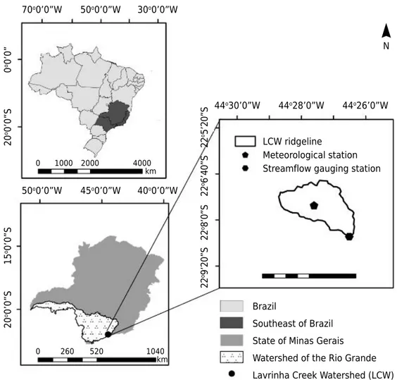
This study was conducted in the Lavrinha Creek Watershed (LCW), located in the domain of the Mantiqueira Range, in the municipality of Bocaina de Minas in the extreme south of Minas Gerais, Brazil. The Mantiqueira Range is a mountainous region along the borders of the states of Minas Gerais, São Paulo, and Rio de Janeiro in southeastern Brazil (Figure 1). The LCW stream drains directly into the Grande River, which is one of the most important Brazilian rivers for hydroelectric generation and water supply for a
significant part of southern Minas Gerais.
The LCW is located between the coordinates of 22° 06’ and 22° 08’ S, and 44° 27’ and
44° 25’ W within the Unidade de Planejamento e Gestão dos Recursos Hídricos (GD01),
a water management planning unit of the Grande River Basin (Figure 1). The watershed
lies at 1,137 to 1,732 m above sea level with a drainage area of about 6.76 km2 and
strongly rolling topography (Menezes et al., 2014; Pinto et al., 2015). The dominant soil class is Inceptsol (Cambissolo Háplico), and the predominant vegetation is Atlantic Forest (ombrophilous forest) (Menezes et al., 2014).
N
Brazil
Southeast of Brazil
State of Minas Gerais
Watershed of the Rio Grande
Lavrinha Creek Watershed (LCW) LCW ridgeline
Meteorological station Streamflow gauging station 44o30’0”W
22
o9’20”
S2
2
o8’0”
S2
2
o6’40”
S2
2
o5’20”
S 44o28’0”W 44o26’0”W
70o0’0”W
0
o0’0”
20
o0’0”S
15
o0’0”S
20
o0’0”S
50o0’0”W 30o0’0”W
50o0’0”W
0 1000 2000 4000 km
1040 520
0 260
km
45o0’0”W 40o0’0”W
Distributed Hydrology Soil-Vegetation Model (DHSVM) and database
In this study, the DHSVM 3.1.2 was used. It should be noted that the DHSVM is a parametric, physically-distributed hydrological model based on water balance and energy budget equations whose solution is run for each grid cell and for each time step in the watershed. Vegetation and soil properties need to be provided for each grid cell; thus, they are spatially distributed within the watershed. Topographical characterization is considered by the
model to control the net solar radiation, rainfall, air temperature, and water flow direction
across the watershed. Simulated water balance in the soil-vegetation system for each grid
cell, which is defined by the resolution of the Digital Terrain Model, is given by equation 1: Σj=1ns ΔSsj + ΔSio + ΔSiu = P – Eio – Eiu – Es – Eto – Etu – Pns
Eq. 1
in which ΔSsj corresponds to soil-water storage in the soil layers (root zone); ΔSio and ΔSiu are
the variations in the overstory and understory interception storages, respectively (rainfall interception); P is the rainfall volume; Es is the soil surface evaporation; Eio, Eiu, Eto, and Etu are
the volumes of overstory and understory evaporation (from interception storage) and overstory and understory transpiration, respectively; and Pns is water percolation from the deeper
root zone. The DHSVM has the following modules: two-layer canopy for evapotranspiration,
soil with multiple layers, overland and sub-surface flows, and water channel routing. A further
mathematical description of the DHSVM can be found in Wigmosta et al. (1994).
We used the Digital Terrain Model (DTM) (outlined between 1,137 and 1,733 m altitude), a soil thickness map, a soil covering map (Atlantic Forest: 63 %, Grassland: 37 %), and soil and moisture zone maps, which will be detailed in the next topic. All these maps were at a 30-m spatial resolution and were georeferenced based on South American Datum (SAD-69), with Universal Transverse Mercator (UTM) coordinates, South 23.
The following parameters were provided for each soil type: Ks - lateral soil saturated
hydraulic conductivity (m s-1), f - rate of exponential decrease in lateral saturated hydraulic
conductivity, IM - maximum infiltration rate (m s-1), αs - soil surface albedo (dimensionless),
K - number of soil layers, Φ - soil porosity (m3 m-3), m - porous size distribution index
(dimensionless), Ψb - pressure at which the air enters the soil (m), θr - residual soil
moisture (m3 m-3
), θc - soil moisture at field capacity (m
3 m-3
), θwp - soil moisture at wilting
point (m3 m-3), D
a - soil bulk density (kg m
-3), and K
v - vertical soil saturated hydraulic
conductivity (m s-1). These parameters were obtained from Junqueira Júnior et al. (2008)
and Oliveira et al. (2014), who mapped several soil physical attributes in the LCW, and
from Kruk (2008) and Cuartas et al. (2012), who developed the first studies related to
applicability of the DHSVM under Brazilian conditions.
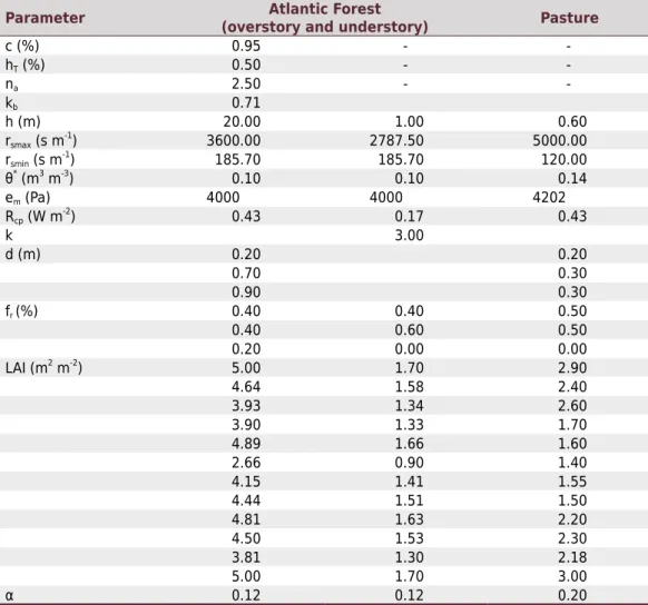
For each vegetation type, the following parameters were provided: c - fractional coverage (%), hT - trunk space (%), na - canopy aerodynamic attenuation coefficient (dimensionless),
kb - radiation attenuation coefficient (dimensionless), h - vegetation height (overstory and understory) (m), rsmax - maximum stomatal resistance (s m-1), rsmin - minimum stomatal
resistance (s m-1), θ* - soil moisture threshold (m3 m-3), e
m - threshold for vapor pressure
deficit above which the stomata close (Pa), Rcp - fraction of photosynthetically active
shortwave radiation (W m-2), k - number of root zones (equal to the number of soil layers),
d - root zone depth (equivalent to the soil layer thickness), fro - overstory root fraction,
fru - understory root fraction, LAIo - overstory monthly leaf area index (from January to
December), LAIu - understory monthly leaf area index (from January to December),
αo - overstory monthly albedo (from January to December), αu - understory monthly
albedo (from January to December). These vegetative parameters were extracted from Wigmosta et al. (1994), Kruk (2008), Ávila (2011), Cuartas et al. (2012), and Mello et al.
(2012). All these parameters remained fixed during DHSVM calibration.
Hourly meteorological datasets were recorded by an automatic weather station in the LCW and were used for DHSVM calibration and validation (Figure 1). This station was
of elevation related to variability of the meteorological parameters, especially rainfall, in the hydrological simulations. In this context, a pluviometer was installed at a higher elevation position of the landscape to record daily rainfall. This dataset showed that the
daily rainfall observed in this position of the watershed was not significantly different
than that observed in the meteorological station (at the average elevation of the LCW).
The hourly weather data sets required by the DHSVM were air temperature (°C), relative humidity (%), wind speed (m s-1), rainfall (m), and shortwave incident radiation (W m-2).
Long wave incident radiation was calculated hourly using the study of Swinbank (1963) as a reference.
Development of soil and moisture zone maps
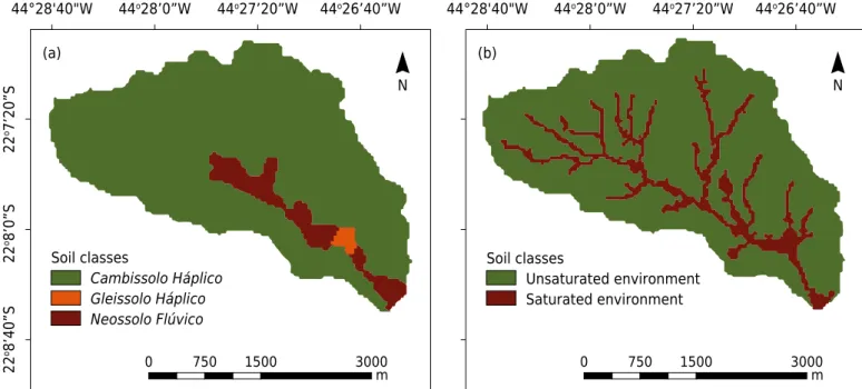
To meet the goals of this study, both a pedological soil map and a moisture zone map were used to describe the hydropedological relationships in the watershed as inputs for running the DHSVM. The soil map was developed by Menezes et al. (2009), who evaluated the morphological, physical, and chemical soil properties to classify them in the LCW and then to proceed with mapping the soil classes. The soil classes in the LCW were
Cambissolos Háplicos (Inceptsols) (92 % of the area), a Gleissolo Háplico (Endoaquents) (1 % of the area), and a Neossolo Flúvico (Udifluvents) (7 % of the area) (Figure 2a).
Gneiss from the Neoproterozoic eon is the parent material of the soils whose weathering-leaching processes resulted in the predominance of shallow Cambissolos Háplicos. These soils are present in areas with mountainous relief and they are mineral soils with A, Bi, and C sequential horizons, along with a shallow solum (A + B horizon) thickness. Gleissolo Háplico is a mineral soil with a gleid horizon immediately below the A horizon, with thickness of less than 0.40 m, or a gleid horizon beginning at the depth of 1.50 m from the surface. The Neossolo Flúvico
consists of soils in formation due to reduced action of pedogenetic processes (weathering).
This soil exhibits insufficient differentiation between horizons, with the A horizon followed
by the C horizon or by rocks (R) (Menezes et al., 2009).
The moisture zone map was obtained by the HAND (Height Above the Nearest Drainage) normalized terrain model, which was introduced by Nobre et al. (2011). The HAND
measures the altimetry difference between a given grid cell point of the DTM and the respective flow point of the nearest drainage network, considering the surface flow path
44°28'40"W
22
o7’20”S (a)
22
o8’0”S
22
o8’40”S
44o28’0”W 44o27’20”W 44o26’40”W
Soil classes
Cambissolo Háplico Gleissolo Háplico Neossolo Flúvico
0 750 1500 3000
m N
44°28'40"W
(b)
44o28’0”W 44o27’20”W 44o26’40”W
Soil classes
Unsaturated environment Saturated environment
0 750 1500 3000
m N
that topologically connects the points of the surface with the drainage network. The result is a grid that represents the DTM normalization in relation to the drainage network. In this
case, all the drainage network points have zero gravitational energy as they are the final
topographical reference points that are directly related to the gravitational drainage of each DTM point. Thus, the points can be placed in equipotential zones whose hydrological
and ecological relevance can be verified (Cuartas et al., 2012).
The HAND model outputs were classified for generating the moisture zone map for the
LCW, following the criteria stated by Nobre et al. (2011). The thresholds considered for this study were: 0 < HAND value < 15 m (for shallow and surface water table level – saturated
zone); and HAND value ≥ 15 m (for deeper water table - unsaturated zone). A contribution
area from which the watercourses flow was defined as 60,000 m2, generating the drainage
network. Finally, the LCW was classified in terms of moisture zones, with 88 % of the area
corresponding to an unsaturated zone and 12 % to a saturated zone (Figure 2b).
In the case of the LCW, for purposes of hydrological simulation, the Cambissolo Háplico and respective parametrization could be linked to unsaturated zones, and the Neossolo Flúvico
and the Gleissolo Háplico to saturated zones, as there was high probability of finding
the respective soil classes in the moisture zones. If this assumption is valid, then the hydrological simulation from both maps will have similar outputs, demonstrating that, in the absence of a pedological soil map, the most common situation, a moisture zone map can be successfully used. It is also noteworthy that only a DTM is required to generate
a moisture zone map, which reduces the costs involved in a field survey.
Calibration and validation strategy for the DHSVM
The streamflows were monitored in the LCW from January 2005 to December 2010 by a
gauging station at the LCW outlet. In this station, a water level sensor was installed to record the depth of the river section (h) in an hourly time step. A stage-discharge curve
[Q = f(h)] was fitted by means of direct discharge measurements throughout the period
mentioned, and it was applied to develop hydrographs after data consistency analysis. Daily average discharges simulated by the DHSVM were then compared with the observed discharges, which were averaged based on hourly values (24 values).
A preliminary sensitivity analysis of the DHSVM parameters was carried out, which showed that this model is very sensitive to both lateral and vertical soil saturated hydraulic conductivities, as well as to the exponential rate of decrease in lateral saturated hydraulic conductivity with soil depth. Thanapakpawin et al. (2007) and Cuartas et al. (2012) corroborate this as they observed the same behavior in their studies. Therefore, the model was calibrated by manually changing each one of the soil parameters. Initially, lateral soil saturated hydraulic conductivity was assumed to be the same value as the vertical soil
saturated hydraulic conductivity in the first soil layer. This parameter was the first to be
calibrated (initial value of Kv = 0.000250 m s
-1), followed by lateral soil saturated hydraulic
conductivity (initial value of Ks = 0.000250 m s
-1) and by the coefficient of variation of
the lateral soil hydraulic conductivity with soil depth (initial value of f = 0.1). For the
simulations, these parameters were first calibrated for the Cambissolo Háplico (92 % of
the area in the case of the soil map) and unsaturated zone (88 % of the area in the case
of the moisture zone map). The same procedure was then used for the Neossolo Flúvico
and the Gleissolo Háplico (8 % of the area in the case of the soil map) and the saturated zone (12 % of the area in the case of the moisture zone map).
into consideration, which defines the regional hydrological year as being from October
of a given year to September of the following year.
The DHSVM was calibrated and validated by searching for the best agreement between the daily
simulated and observed discharges in the LCW. After obtaining a good visual fit, the calibration procedure was refined by means of maximization of the objective functions, specifically, the
coefficient of determination (R2
) and the Nash-Sutcliffe coefficient (E) (Equations 2 and 3). Σi=1N (Qoi – Qo)(Qsi – Qs)
Σi=1N [(Qoi – Qo)2]0.5[(Qsi – Qs)2]0.5
R2 =
2
Eq. 2
E = 1.0 –
Σi=1N (Qoi – Qsi)2
Σi=1N (Qoi – Qo)2 Eq. 3
in which, Qoi = observed discharge in day i (m3 s-1); Qsi = simulated discharge in day i
(m3 s-1);
Qo = average observed discharge (m3 s-1);
Qs = average simulated discharge
(m3 s-1); and N = number of days.
The R2 and E values, respectively, greater than 0.50 means a model qualified as “acceptable”
(Van Liew et al., 2003; Moriasi et al., 2007). In contrast, Safeeq and Fares (2012) suggest that 0.35 < E < 0.50 indicates “mean” performance, 0.50 < E < 0.70 indicates “good” performance, and E greater than 0.70 indicates “very good” performance of the model.
RESULTS AND DISCUSSION
DHSVM calibration based on soil and moisture zone maps
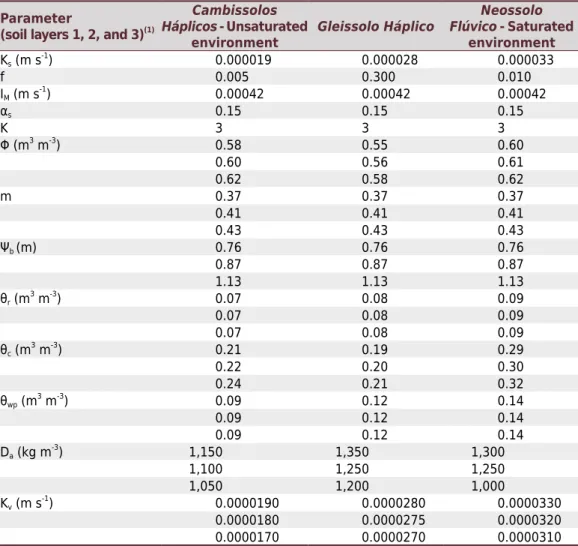
Based on the previous DHSVM sensitivity analysis, the parameters of vertical and lateral soil saturated hydraulic conductivity and the exponential rate of decrease in lateral
saturated hydraulic conductivity with soil depth were verified one by one for model calibration. Tables 1 and 2 show the final soil calibrated parameters based on the soil
map (columns 2, 3, and 4, Table 1) and the moisture zone map (columns 2 and 4, Table 1),
and the final vegetative parameters (Table 2).
The precision statistics obtained by DHSVM calibration and validation based on the soil and moisture zone maps were presented in the table 3, which allow analysis of performance of
the hydrological model for streamflow simulations in the LCW. First, the statistical indices
were similar for the calibration and validation phases. Taking the studies of Van Liew et al. (2003), Moriasi et al. (2007), and Safeeq and Fares (2012) as references for these precision statistics, both simulations (soil and moisture zone maps) can be considered satisfactory from the hydrological simulation point of view. Other studies conducted using the DHSVM, like the studies of Thanapakpawin et al. (2007) and Cuartas et al. (2012), obtained a
Nash-Sutcliffe coefficient ranging from -2.22 to 0.79 and 0.14 to 0.76 for calibration and
validation daily discharges, respectively. Thus, the results obtained in the present study demonstrated that the DHSVM performed well for the geomorphological characteristics of the Mantiqueira Range region using both types of maps, comparable to other studies
conducted for different geomorphological and weather characteristics.
The Nash-Sutcliffe coefficient was slightly greater for simulations based on the moisture zone map. A possible explanation for that result is that some areas classified and mapped as
Inceptisols (Cambissolos Háplicos) have hydrological behavior similar to the Neossolo Flúvico, especially near the drainage network (Figure 2a), which tended to generate a lower amount
of overland flow in the simulations based on the moisture zone map.
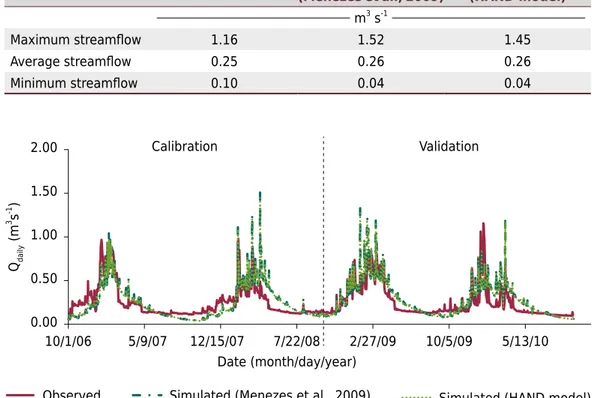
The observed and simulated hydrographs (using both soil and moisture zone maps as
had trouble simulating baseflow during the dry season (underestimates) and the peak flows (overestimates) during the wet season. In this context, further results are shown in
table 4, consisting of the observed and simulated data (using both maps) of maximum, average, and minimum discharges throughout the period studied (validation and calibration). Average annual observed and simulated discharges had similar and satisfactory values;
however, for extreme discharges (maximum and minimum values), greater difficulty can
be observed for simulations with the DHSVM, regardless of the map used (Figure 3).
Observed daily frequency discharge curve and simulated daily frequency discharge curves
(the latter based on both soil and moisture zone maps) are presented in figure 4. In the simulated discharges, only very slight differences could be visually observed. In general, the results found for the LCW showed a good fit of the simulated daily frequency discharge
curves to that observed for both calibration and validation (Figure 4). These results are supported by the discharges simulated with 10 and 90 % of exceeding frequencies (Q10 %
and Q90 %). The observed Q90 % was about 0.51 m
3 s-1, whereas the ones simulated using
both maps were 0.53 m3 s-1. Considering Q
10 %, the observed and simulated (based on
both maps) values were 0.12 and 0.08 m3 s-1, respectively.
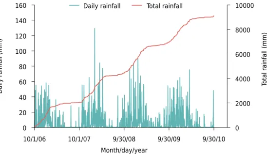
Good agreement was found between the observed and simulated (using both maps) accumulated
daily runoff outputs for calibration and validation (Figure 5). The accumulated runoff observed was 4,670 mm and simulated runoff based on both maps was 4,898 mm, which corresponded
to 51 and 54 % of the total precipitation, respectively, over the period studied (Figure 6).
Table 1. Final Distributed Hydrology Soil Vegetation Model soil parameter values for the Lavrinha Creek Watershed, considering the soil map and zone map
Parameter
(soil layers 1, 2, and 3)(1)
Cambissolos
Háplicos - Unsaturated
environment
Gleissolo Háplico
Neossolo
Flúvico - Saturated
environment Ks (m s
-1) 0.000019 0.000028 0.000033
f 0.005 0.300 0.010
IM (m s
-1) 0.00042 0.00042 0.00042
αs 0.15 0.15 0.15
K 3 3 3
Φ (m3 m-3) 0.58 0.55 0.60
0.60 0.56 0.61
0.62 0.58 0.62
m 0.37 0.37 0.37
0.41 0.41 0.41
0.43 0.43 0.43
Ψb (m) 0.76 0.76 0.76
0.87 0.87 0.87
1.13 1.13 1.13
θr (m3 m-3) 0.07 0.08 0.09
0.07 0.08 0.09
0.07 0.08 0.09
θc (m
3 m-3) 0.21 0.19 0.29
0.22 0.20 0.30
0.24 0.21 0.32
θwp (m
3 m-3) 0.09 0.12 0.14
0.09 0.12 0.14
0.09 0.12 0.14
Da (kg m
-3) 1,150 1,350 1,300
1,100 1,250 1,250
1,050 1,200 1,000
Kv (m s -1
) 0.0000190 0.0000280 0.0000330
0.0000180 0.0000275 0.0000320
0.0000170 0.0000270 0.0000310
(1)
Ks: lateral soil saturated hydraulic conductivity, f: rate of exponential decrease in lateral saturated hydraulic
conductivity, IM: maximum infiltration rate, αs: soil surface albedo, K: number of soil layers, Φ: soil porosity, m: porous
size distribution index, Ψb: pressure at which the air enters the soil, θr: residual soil moisture, θc: soil moisture at field
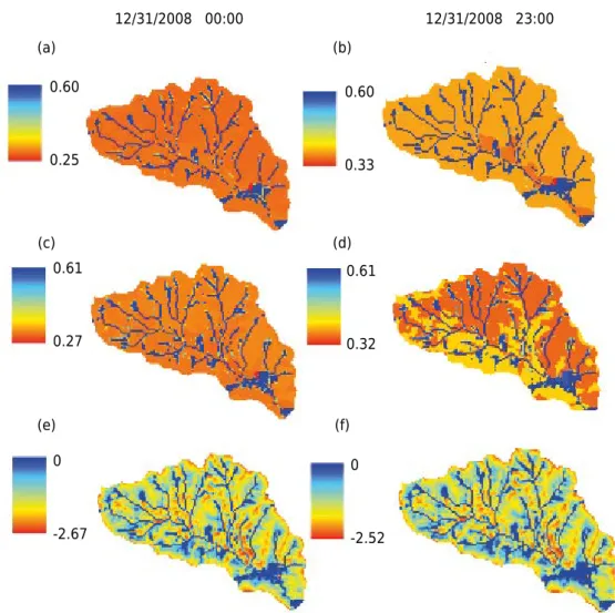
Simulation of the spatial distribution of soil moisture and water table depth by the DHSVM
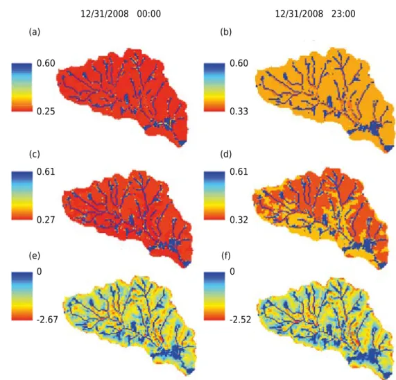
Simulated soil moisture and water table depth maps based on the soil map are shown in
figure 7, and those based on the moisture zone map, in figure 8. These maps were simulated
for the rainfall event recorded on December 31, 2008, considering the behavior of these hydrological variables in the watershed before and after occurrence of the event. This rainfall event began at 4:00 p.m. and had an accumulated value of 59 mm up to 11:00 p.m. Thus, it is plausible to assume that the hydrological variables simulated by the DHSVM at 0:00 and 23:00 (December 31) represented the hydrological conditions in the LWC reasonable
well, especially the effect of temporal variability of the rainfall on the simulations by the
DHSVM for each of the maps used in this study (soil and moisture zone maps).
Table 2. Final Distributed Hydrology Soil Vegetation Model vegetation parameter values for the Lavrinha Creek Watershed
Parameter Atlantic Forest
(overstory and understory) Pasture
c (%) 0.95 -
-hT (%) 0.50 -
-na 2.50 -
-kb 0.71
h (m) 20.00 1.00 0.60
rsmax (s m
-1) 3600.00 2787.50 5000.00
rsmin (s m
-1) 185.70 185.70 120.00
θ* (m3 m-3) 0.10 0.10 0.14
em (Pa) 4000 4000 4202
Rcp (W m
-2) 0.43 0.17 0.43
k 3.00
d (m) 0.20 0.20
0.70 0.30
0.90 0.30
fr (%) 0.40 0.40 0.50
0.40 0.60 0.50
0.20 0.00 0.00
LAI (m2 m-2) 5.00 1.70 2.90
4.64 1.58 2.40
3.93 1.34 2.60
3.90 1.33 1.70
4.89 1.66 1.60
2.66 0.90 1.40
4.15 1.41 1.55
4.44 1.51 1.50
4.81 1.63 2.20
4.50 1.53 2.30
3.81 1.30 2.18
5.00 1.70 3.00
α 0.12 0.12 0.20
c: fractional coverage, hT: trunk space, na: canopy aerodynamic attenuation coefficient, kb: radiation attenuation
coefficient, h: vegetation height (overstory and understory), rsmax: maximum stomatal resistance, rsmin: minimum
stomatal resistance, θ*
: soil moisture threshold, em: threshold for vapor pressure deficit above which the
stomata close, Rcp: fraction of photosynthetically active shortwave radiation, k: number of root zones, d: root
zone depth, fr: root fraction, LAI: monthly leaf area index, α: monthly albedo.
Table 3. Distributed Hydrology Soil Vegetation Model performance using the soil map and moisture zone map
Menezes et al. (2009) HAND model
E R2
E R2
Daily calibration 0.52 0.62 0.56 0.62
As soon as the rainfall ended, a slight increase in soil moisture spatial variability was
observed in the first (0.00-0.20 m) and second (0.20-0.70 m) soil layers in the LCW (Figures 7a, 7b, 7c, 7d, 8a, 8b, 8c, and 8d) due to the first effects of the rainfall on the
soil surface. For both soil and moisture zone maps, the DHSVM simulated soil moisture up to 0.33 m3 m-3 for the first soil layer (Figures 7b and 8b), and 0.32 m3 m-3 for the soil
map and 0.33 m3 m-3 for the moisture zone map for the second layer (Figures 7d and 8d). 0.00
0.50 1.00 1.50 2.00
10/1/06 5/9/07 12/15/07 7/22/08 2/27/09 10/5/09 5/13/10 Date (month/day/year)
Calibration
Qdaily
(m
3 s -1 )
Validation
Observed Simulated (Menezes et al., 2009) Simulated (HAND model)
Figure 3. Observed and simulated hydrographs for the Lavrinha Creek Watershed (calibration and validation) for the soil map and moisture zone map.
Table 4. Observed and simulated values (based on the soil and moisture zone maps) of maximum, average, and minimum streamflow, from October 2006 to September 2010
Daily streamflow Observed Simulated (Menezes et al., 2009)
Simulated (HAND model) m3
s-1
Maximum streamflow 1.16 1.52 1.45
Average streamflow 0.25 0.26 0.26
Minimum streamflow 0.10 0.04 0.04
0.00 0.20 0.40 0.60 0.80 1.00 1.20 1.40 1.60
0.00 0.10 0.20 0.30 0.40 0.50 0.60 0.70 0.80 0.90 1.00
St
re
amflow (m
3 s -1 )
Duration curves
Observed streamflow
Simulated streamflow (Menezes et al., 2009)
Simulated streamflow (HAND model)
Figure 4. Duration curves of the observed and simulated daily streamflow in the Lavrinha Creek
The simulated water table depth demonstrated that this hydrological variable was shallower (closer to the surface) for both input maps (Figures 7e, 7f, 8e, and 8f). The maximum depth changed from -2.67 to -2.52 m (Figures 7e and 7f) and from -2.72 to -2.57 m (Figures 8e and 8f) using the soil and moisture zone maps, respectively. In addition, we found that the water table depth had less spatial variability than soil moisture.
The amount of rain in December 2008 was above average in most of the state of Minas Gerais, especially in the south. A total of 438 mm was observed in the LCW, which was
200 mm greater than normal rainfall according to the Boletim Climanálise - CPTEC
(Climanálise, 2008). Thus, soil moisture in the LCW exhibited greater values throughout
December 2008, which means that this previous condition defined the initial hydrology of
the system and had a crucial role in the response to this rainfall event in the watershed.
There were small differences in soil moisture and water table depth, before and after the rainfall event (Figures 7 and 8), with an increase in overland flow.
Similar spatial distribution of the hydrological variables was showed because of
the predominance of the Cambissolos Háplicos (92 % of the LCW area) and, in fact,
predominance of the unsaturated zone due to the deeper water table (88 % of the
Observed runoff
Simulated runoff (Menezes et al., 2009)
Simulated runoff (HAND model)
0 1000 2000 3000 4000 5000
10/1/06 10/1/07 9/30/08 9/30/09 9/30/10
R
unoff (mm)
Month/day/year
Figure 5. Observed and simulated cumulative daily runoff in the Lavrinha Creek Watershed, from
October 2006 to September 2010, based on the soil map and moisture zone map.
0 2000 4000 6000 8000 10000
0 20 40 60 80 100 120 140 160
10/1/06 10/1/07 9/30/08 9/30/09 9/30/10
To
tal rainfall (mm)
Daily rainfall (mm)
Month/day/year
Daily rainfall Total rainfall
LCW area) (Figures 7 and 8). However, the good results generated by the DHSVM using the HAND model map as input can be explained by the equivalence of the saturated
zones defined by HAND procedures (Figures 8a, 8b, 8c, and 8d) with the shallow water
table (Figure 2b) in the LCW. The results demonstrated that the model was capable of simulating the initial conditions close to saturation in the LCW, which was most of the area found in the drainage network, where it simulated both the greatest soil moisture and the shallowest water table.
The results found in this study are highly relevant because they showed that the moisture zone map developed by the HAND model can be used for hydrological simulations in mountainous watersheds like the LCW, given that most mountainous watersheds do not have a detailed soil map. It is also important to emphasize that soil surveying under
field conditions is laborious, demanding time and field and laboratory analyses; this
type of survey also is on a scale that is generally not adequate for small catchments, limiting the quality of the hydrological simulations on a micro-scale. The LCW is one of the only hydrological units in the Mantiqueira Range with a very good soil map based on a detailed soil survey, which allowed us to appropriately compare the hydrological simulation outputs from the DHSVM.
It should be emphasized that running a hydrological simulation with the DHSVM requires many fundamental input variables and parameters related to the area, weather and discharge data
sets with a detailed time interval, adequate soil and land-use maps, and a fine resolution of the Digital Terrain Model. The LCW has been a scientific laboratory, with other studies
(a)
(c)
(e)
(b) 12/31/2008 00:00
0.60
0.25
0.61
0.27
0.61
0.32
0
-2.67
0
-2.52 0.60
0.33
12/31/2008 23:00
(d)
(f)
Figure 7. Soil moisture content in the 0.00-0.20 m (a, b) and 0.20-0.70 m (c, d) layers (m3 m-3
that involved soils, climate, water table monitoring, water quality and sediment transport, groundwater recharge, and water balance (Junqueira Júnior et al., 2008; Menezes et al., 2009; Ávila et al., 2010; Mello et al., 2012; Oliveira et al., 2014; Menezes et al., 2014; Pinto et al., 2015). This served as a background for conducting DHSVM calibration, allowing comparisons between a soil map and a moisture zone map as inputs for the model. In addition, it is important to highlight that the LCW represents the geomorphological feature of small variability in soil classes, with the Inceptisol (Cambissolo Háplico) predominant in almost the entire area. This situation, which is expected in most of the region of the Mantiqueira Range, made application of the HAND model easier. Thus, the procedure tested in this study can also be further analyzed in a comprehensive future study with greater variability of
soil classes, with the soil map developed from field soil surveys, and with hydrological and
weather data sets available for DHSVM calibration and validation.
CONCLUSIONS
The hydrological simulations conducted with the DHSVM based on a detailed soil map and moisture zone map characterized by the HAND model, satisfactorily represented the hydrological behavior of the LCW, according to the indices of statistical precision.
Comparing the results of the simulations based on both maps, only slight differences in the simulated discharges, runoff, soil moisture, and water table depth maps could be
observed, meaning that the results of the HAND model can be applied in connection with the DHSVM.
(a)
(c)
(e)
(b) 12/31/2008 00:00
0.60
0.25
0.60
0.33
0.61
0.27
0.61
0.32
0
-2.67
0
-2.52
12/31/2008 23:00
(d)
(f)
Figure 8. Soil moisture content in the 0.00-0.20 m (a, b) and 0.20-0.70 m (c, d) layers (m3 m-3
The results of this study show that it is possible to use moisture zone maps instead of a soil map in hydrological simulations with the DHSVM. In addition, in some cases, the HAND model can generate further details, depending on the DTM resolution, which, in turn, can result in more detailed hydrological output maps (soil moisture and water table depth). However, this study with the DHSVM also demonstrated that providing soil samples in
the different moisture zones for estimation of the parameters required by the DHSVM is
indispensable, and this can only be done based on existing soil surveys for the area studied.
Considering the number of parameters and the difficulty of characterizing them on the field level, the results obtained in this study are of great importance for future DHSVM
users, as well as for studies in mountainous regions in southeast Brazil, especially in the domain of the Mantiqueira Range.
ACKNOWLEGMENTS
The authors would like to thank FAPEMIG (PPM X 00415-16) and CAPES for the Sandwich
Doctorate Program scholarship (Process 99999.014035/2013-08) for the first author.
REFERENCES
Alvarenga LA, Mello CR, Colombo A, Cuartas LA, Bowling LC. Assessment of land cover change on the hydrology of a Brazilian headwater watershed using the distributed Hydrology-Soil-Vegetation
Model. Catena. 2016;143:7-17. https://doi.org/10.1016/j.catena.2016.04.001
Ávila LF. Balanço hídrico em um remanescente de Mata Atlântica da Serra da Mantiqueira, MG [tese]. Lavras: Universidade Federal de Lavras; 2011.
Ávila LF, Mello CR, Silva AM. Estabilidade temporal do conteúdo de água em três condições
de uso do solo, em uma bacia hidrográfica da região da Serra da Mantiqueira, MG.
Rev Bras Cienc Solo. 2010;34:2001-9. https://doi.org/10.1590/S0100-06832010000600024
Bowling LC, Lettenmaier DP. The effects of forest roads and harvest on catchment hydrology
in a mountainous maritime environment. In: Wigmosta MS, Burges SJ, editors. Land use and
watersheds: human influence on hydrology and geomorphology in urban and forest areas.
Washington: American Geophysical Union; 2001. p.145-64.
Climanálise. Boletim de monitoramento e análise climática [internet]. Cachoeira Paulistas; 2008 [acesso: 17 Nov 2014]. Disponível em: http://climanalise.cptec.inpe.br/~rclimanl/boletim/ pdf/pdf08/dez08.pdf.
Cuartas LA. Estudo observacional e de modelagem hidrológica de uma micro-bacia em floresta
não perturbada na Amazônia central [tese]. São José dos Campos: Instituto Nacional de Pesquisas Espaciais; 2008.
Cuartas LA, Tomasella J, Nobre AD, Nobre CA, Hodnett MG, Waterloo MJ, Oliveira SM,
Randow RC, Trancoso R; Ferreira M. Distributed hydrological modeling of a micro-scale rainforest watershed in Amazonia: Model evaluation and advances in calibration using the new HAND
terrain model. J Hydrol. 2012;462-463:15-27. https://doi.org/10.1016/j.jhydrol.2011.12.047 Gharari S, Hrachowitz M, Fenicia F, Savenije HHG. Hydrological landscape classification: investigating the performance of HAND based landscape classifications in a central European meso-scale
catchment. Hydrol Earth Syst Sci. 2011;15:3275-91. https://doi.org/10.5194/hess-15-3275-2011
Junqueira Júnior JA, Silva AM, Mello CR, Pinto DBF. Continuidade espacial de atributos
físico-hídricos do solo em sub-bacia hidrográfica de cabeceira. Cienc Agrotec. 2008;32:914-22.
https://doi.org/10.1590/S1413-70542008000300032
Kruk NS. Sistema hidrometeorológico proposto para previsão de eventos extremos numa microbacia
de topografia complexa [tese]. São José dos Campos: Instituto Tecnológico de Aeronáutica; 2008.
Menezes MD, Junqueira Júnior JA, Mello CR, Silva AM, Curi N, Marques JJ. Dinâmica hidrológica de duas nascentes, associada ao uso do solo, características pedológicas e atributos
físico-hídricos na sub-bacia hidrográfica do Ribeirão Lavrinha - Serra da Mantiqueira (MG). Sci
For. 2009;82:175-84.
Menezes MD, Silva SHG, Mello CR, Owens PR, Curi N. Solum depth spatial prediction comparing conventional with knowledge-based digital soil mapping approaches. Sci Agric. 2014;71:316-23. https://doi.org/10.1590/0103-9016-2013-0416
Moriasi DN, Arnold JG, Van Liew MW, Bingner RL, Harmel RD, Veith TL. Model evaluation
guidelines for systematic quantification of accuracy in watershed simulations. Trans ASABE.
2007;50:885-900. https://doi.org/10.13031/2013.23153
Nobre AD, Cuartas LA, Hodnett M, Rennó CD, Rodrigues G, Silveira A, Waterloo M, Saleska S. Height above the nearest drainage - a hydrologically relevant new terrain model. J Hydrol.
2011;404:13-29. https://doi.org/10.1016/j.jhydrol.2011.03.051
Oliveira AS, Silva AM, Mello CR, Alves GJ. Stream flow regime of springs in the
Mantiqueira Mountain Range region, Minas Gerais State. Cerne. 2014;20:343-9. https://doi.org/10.1590/01047760201420031268
Pereira DR, Almeida AQ, Martinez MA, Rosa DRQ. Impacts of deforestation on water balance components of a watershed on the Brazilian East Coast. Rev Bras Cienc Solo. 2014;38:1350-8. https://doi.org/10.1590/S0100-06832014000400030
Pinto LC, Zinn YL, Mello CRD, Owens PR, Norton LD, Curi N. Micromorphology and pedogenesis of mountainous Inceptisols in the Mantiqueira range (MG). Cienc Agrotec. 2015;39:455-62. https://doi.org/10.1590/S1413-70542015000500004
Price K. Effects of watershed topography, soils, land use, and climate on baseflow hydrology in humid
regions: a review. Progr Phys Geogr. 2011;35:465-92. https://doi.org/10.1177/0309133311402714
Rennó CD, Nobre AD, Cuartas LA, Soares JV, Hodnett MG, Tomasella J, Waterloo MJ. HAND, a new terrain descriptor using SRTM-DEM: mapping terra-firme rainforest environments in Amazonia.
Rem Sens Environ. 2008;112:3469-81. https://doi.org/10.1016/j.rse.2008.03.018
Safeeq M, Fares A. Hydrologic response of a Hawaiian watershed to future climate change scenarios. Hydrol Proc. 2012;26:2745-64. https://doi.org/10.1002/hyp.8328
Swinbank WC. Long-wave radiation from clear skies. Q J Roy Meteorol Soc. 1963;89:339-48.
https://doi.org/10.1002/qj.49708938105
Thanapakpawin P, Richey J, Thomas D, Rodda S, Campbell B, Logsdon M. Effects of land
use change on the hydrologic regime of the Mae Chaem river basin, NW Thailand. J Hydrol.
2007;334:215-30. https://doi.org/10.1016/j.jhydrol.2006.10.012
Van Liew MW, Arnold JG, Garbrecht JD. Hydrologic simulation on agricultural watersheds: choosing between two models. Trans ASAE. 2003;46:1539-51. https://doi.org/10.13031/2013.15643
Wigmosta MS, Vail LW, Lettenmaier DP. A distributed hydrology‐vegetation model for complex