Mariana Côrte-Real Marques Pedro
Licenciada em Engenharia Electrotécnica e de Computadores
Modelling of Shading Effects in Photovoltaic
Optimization
Dissertação para obtenção do Grau de
Mestre em Engenharia Electrotécnica e de Computadores
Orientador: João Murta Pina, Professor Doutor, FCT-UNL
Júri:
A
CKNOWLEDGEMENTS
First of all, I would like to express my gratitude to my supervisor, Professor João Murta Pina, for all his support and availability during the elaboration of this dissertation. His opinions provided me with direction, motivating me to pursue the best possible outcome.
I would also like to thank the Faculty of Sciences and Technology of Nova University of Lisbon, in particular to the Department of Electrical Engineering, for providing me with the relevant conditions (equipment, infrastructure, etc.) necessary to develop the work that lead to this dissertation. I would also like to take the chance to thank all my lecturers from whom I learned and ultimately grew during the past years.
I would also like to thank my family for the support they provided through my entire life. In particular, I must mention my father who patiently provided me with guidance on how to structure my thought and my writing in order to produce an important document as this one.
A
BSTRACT
The use of photovoltaic systems as a source of power supply has entered a maturity phase. Nevertheless, there is still some room for improvement in certain areas, such as the accurate estimation of power output production during the project stage.
There are different types of shading with distinct effects on photovoltaic energy produc-tion. These differences need to be taken into account when projecting a PV installaproduc-tion. The ECEN2026 is a PV module model, that enables the simulation of any existent solar panel, according to a set of parameters, which can be compared with real world installations, providing a mean to study the feasibility of hypothetical installation.
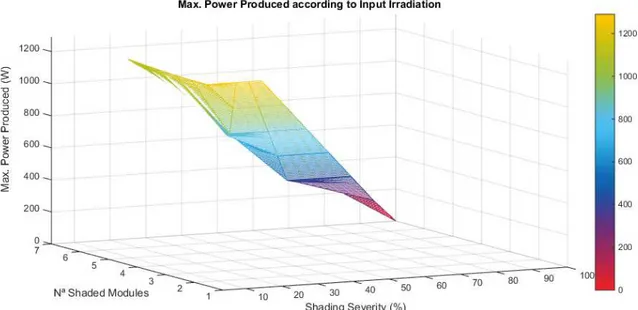
The implementation and simulation of this model generates several outputs. In the presented context, an expression can be obtained, which correlates the annual power production with the severity of shading and the number of shaded panels. It also allows the plot of the IV and PV characteristic curves, aiming to optimize the maximum output power and, using different shading situations, to validate the model. R
The model validation is possible due to the comparison between the obtained simula-tion results and practical implementasimula-tions. One limitasimula-tion of this model is the impossibility to simulate partly shaded modules.
R
ESUMO
A utilização de sistemas fotovoltaicos como fonte de fornecimento de energia encontra-se atualmente numa faencontra-se deencontra-senvolvida. No entanto há espaço para melhoria em determi-nadas áreas, como a precisão na estimativa de potência produzida aquando do projeto de uma instalação.
Existem diferentes tipos de sombreamento que afetam de diferente forma a produção de energia fotovoltaica. Estes devem ser tidos em conta na fase de projeto. O ECEN2026 é um modelo de módulo fotovoltaico que permite a simulação de qualquer painel solar existente, com base num grupo de parâmetros, que pode ser comparado com instalações reais, fornecendo uma forma de estudar a viabilidade de instalações hipotéticos.
A implementação e simulação deste modelo gera vários resultados possíveis. Neste contexto, uma expressão é gerada, correlacionando a produção energética anual com a severidade de sombreamento e número de módulos sombreados. Este permite também o desenho de curvas corrente-tensão e potência-tensão, com o objetivo de otimizar em tempo real a potência produzida e, usando diferentes situações de sombreamento, validar o modelo em si.
A validação do modelo é possível devido à comparação entre os resultados de simula-ção obtidos e implementações práticas. Uma limitasimula-ção do mesmo é a impossibilidade de simular painéis parcialmente sombreados.
C
ONTENTS
Contents xi
List of Figures xiii
List of Tables xvii
1 Introduction 1
1.1 Motivation . . . 1
1.2 Objectives . . . 2
1.3 Contribution to the Domain . . . 2
1.4 Structure of the Thesis . . . 3
2 State of the Art 5 2.1 Shading Influence on Photovoltaic Systems . . . 5
2.1.1 Types of Shading Effects on the Photovoltaic System . . . 5
2.1.2 Effects of Shading on Photovoltaic Systems . . . 6
2.2 Modelling Solar Systems . . . 10
2.2.1 PN Juntion . . . 10
2.2.2 Mathematical Model and Equivalent Circuit of a PV Cell . . . 11
2.3 Strategies to Optimize the Shading Effect on Solar Panels . . . 16
2.3.1 Evolution in Optimization in the Past Decades . . . 16
2.3.2 Use of Diodes to Compensate the Shading Effect on Solar Panels . 22 2.4 Methods for Calculating the Shade Factor for a Photovoltaic System . . . . 24
2.4.1 Calculations Based on Observation . . . 25
2.4.2 Computer Aided Calculations and Software . . . 28
2.4.3 Shading Simulation Software Review . . . 31
3 Implementation Simulations in Simulink 37 3.1 Introduction to the ECEN2026 Model . . . 37
3.1.1 Specifications of the Model . . . 38
3.1.2 Simulink Implementation . . . 38
3.2 Simulations . . . 41
3.2.2 Simulation and Study of IV and PV Characteristic Curves for
Differ-ent Cases of Shading . . . 43
3.2.3 Development of the Power Output Expression of a Specific PV In-stallation According to Shade Variation . . . 45
3.2.4 Determination of the Annual Energy Production of a Single PV Module Assuming a Previously Defined Shade . . . 50
3.2.5 Comparison between the impact of a calculated Shade Factor on the production of an installation with the one simulated . . . 57
4 Experimental Results Testing Shadings on Photovoltaic Panels 67 4.1 Test of Isolated Modules . . . 67
4.1.1 Evaluation of IV and PV Curves on Photovoltaic Modules . . . 67
4.1.2 Experiment 1 . . . 69
4.1.3 Experiment 2 . . . 74
4.1.4 Remarks on the Outputs of Experiments 1 and 2 . . . 76
4.2 Test of Grid-connected Modules . . . 77
4.2.1 Study of the Power Production on a two Module Installation . . . . 77
4.2.2 Experiment 3 - No Shade Cast on the Installation: . . . 81
4.2.3 Experiment 4 - A Single Module With Soft Shading cast upon it: . . 82
4.2.4 Experiment 5 - One Module Partly Soft Shaded: . . . 84
4.2.5 Experiment 6 - One Module Partly Hard Shaded: . . . 85
4.2.6 Remarks on the Outputs of Experiments 3 to 6 . . . 86
5 Conclusions and Future Work 87 5.1 Conclusions . . . 87
5.2 Future Work . . . 89
Bibliography 91
L
IST OF
F
IGURES
2.1 Cell hard shading examples. Source: Sargosis Solar & Electric, 2014. . . 6
2.2 Hot spot heating. Source: Honsberg and Bowden, 2011. . . 7
2.3 Effects on IV characteristic curves on solar systems taking into account the type of shade suffered. Source: Sargosis Solar & Electric, 2014. . . 8
2.4 Effects on PV characteristic curves on solar systems taking into account the type of shade suffered. Source: Sargosis Solar & Electric, 2014. . . 10
2.5 PN junction of a solar cell. Source: Masters, 2004. . . 11
2.6 Circuit linking a solar cell to a load. Source: Masters, 2004. . . 11
2.7 Equivalent circuit of a PV cell. Source: Masters, 2004. . . 12
2.8 PV cell model examples drawn using a circuit simulator software. . . 12
2.9 Single-diode model - equivalent circuit of a PV cell. Source: Marnoto, Sopian, Daud, Algoul, and Zaharim, 2007. . . 13
2.10 Short-circuit current and open-circuit voltage. Source: Masters, 2004. . . 15
2.11 Photovoltaic IV relationship for "dark" (no sunlight) and "light" (illuminated cell). Source: Masters, 2004. . . 16
2.12 Conventional grid-tie PV system with central inverter. Source: Tsao, 2010. . . 17
2.13 Micro-inverters application and power saving example. Source: Canterbury Power Solutions, 2012. . . 18
2.14 Power optimizers installation examples. Source: Tsao, 2010. . . 19
2.15 Solar dual-axis tracker application example. Source: Queensland Windmill & Solar, 2008. . . 20
2.16 Example of installation without backtracking technology. Source: Sistemas Digitales de Control 2002, S.L., 2014. . . 21
2.17 Installation using backtracking technology. Source: Sistemas Digitales de Con-trol 2002, S.L., 2014. . . 21
2.18 Bypass and blocking diode application. Source: Storr, 2014. . . 23
2.19 Sun path diagram of shading from objects over 10 m away. Source: (MCS), 2012. 26 2.20 Sun path diagram of shading from objects within 10 m of distance from the away. Source: (MCS), 2012. . . 27
2.22 Module positioning analysis on PVCad. Source:Controlling software for
photo-voltaics - PVCAD2015. . . 33
2.23 Archelios report on shadow analysis. Source:Archelios PRO. . . 34
2.24 Simulation with power optimizers in 3D mode. Source: Zipp, 2014. . . 35
2.25 Solmetric Suneye solar reading. Source: Home Power Inc., 2015. . . 35
2.26 Easy solar app - PV designing tool. Source: Zipp, 2014. . . 36
3.1 Equivalent circuit of a PV cell used on the ECEN2026 model. Source: Marnoto, Sopian, Daud, Algoul, and Zaharim, 2007. . . 38
3.2 Current and voltage module inputs designed using Simulink . . . 38
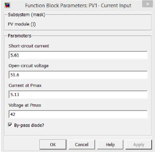
3.3 Parameters of the PV current and voltage input modules designed. . . 39
3.4 Parameters of the PV current-input module mask designed. . . 40
3.5 Voltage-input module undermask subsystem design. . . 40
3.6 PV installation with seven modules designed using Simulink. . . 42
3.7 PV installation with a single module designed using Simulink. . . 43
3.8 PV installation with two PV modules designed using Simulink. . . 43
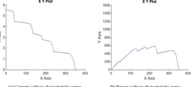
3.9 Case 1: Simulink XY plot of the IV and PV curves for a PV installation with two modules. . . 44
3.10 Case 2: Simulink XY plot of the IV and PV curves for a PV installation with seven modules. . . 44
3.11 Explanatory diagram of the process used on scrip A.2 (steps 1 to 4). . . 46
3.12 Correlation between maximum power produced, number of shaded modules and shade severity plotted using MATLAB. . . 47
3.13 Fit of the correlation between maximum power produced, number of shaded modules and shade severity plotted using MATLAB’c fitting tool - Cftoll. . . 48
3.14 Sun path chart of Lisbon 2015 designed usingUniversity of Oregon Sun Path Chart Programavailable online. Source: University of Oregon, Solar Radiation Monitoring Laboratory, 2007. . . 52
3.15 Sun path chart of Lisbon 2015 with shade cast byobject 1. . . 53
3.16 Parameters of the PV voltage-input module mask designed. Source: University of Oregon, Solar Radiation Monitoring Laboratory, 2007. . . 53
3.17 Power production from January for diffuse or zero irradiance cast upon the module when shaded byobject 1. . . 54
3.18 Monthly power production estimation without shade - simulated using Simulink and plotted using MATLAB. . . 55
3.19 Monthly power production estimation considering diffuse or zero irradiation is input on the installation when shaded byobject 1. . . 55
3.20 Comparison between Images (a) and (b) to design a new sun path diagram with 84 segments, essential to the calculus of the SF. . . 58
3.21 New solar path chart created by comparison of figures 3.20a and 3.20b. . . 59
3.23 Display ofObject 2on the sun path chart. . . 61 3.24 Display ofObject 3on the sun path chart. . . 62 3.25 SF calculus ofObject 2using the solar path chart developed for this propose. . 63 3.26 SF calculus ofObject 3using the solar path chart developed for this propose. . 64 4.1 Diagram of the circuit composed of a photovoltaic module, designed using
Simulink. . . 69 4.2 IV characteristic curve plotted using the values input to an Excel spreadsheet. 70 4.3 IV curve family for module, for a 25oC cell temperature, as a function of irradiace. 71 4.4 IV Curve family for Module HIP-215NHE5 for a 1000 W/m2irradiance as a
function of temperature. . . 71 4.5 PV characteristic curve resulting from the values input to the Excel spreadsheet. 72 4.6 Nominal electrical data for the SANYO HIP-xxxNHE5 module family (relevant
data for the tested model contained in the "215" column). . . 73 4.7 IV characteristic curve plotted using the values input to an Excel spreadsheet. 75 4.8 PV characteristic curve plotted using the values input to an Excel spreadsheet. 75 4.9 Shaded experiment 3 - Two module installation configuration with Micro-inverter. 77 4.10 Illustrations of shaded cases B to D, where different shading situations are
simulated. . . 78 4.11 Diagram of the setup used to gather information from the installation to the
APS EMA. Source: CivicSolar, 2015 . . . 79 4.12 Layout of experiment 3 - Installation with two PV panels and a micro-inverter
with no shade cast upon them. . . 81 4.13 EMA real-time data screen production for experiment 3. . . 81 4.14 Simulink simulation of experience 3. . . 82 4.15 Layout of experiment 4 - Photovoltaic installation with a translucent fabric
casting soft shade on totality of one module surface. . . 83 4.16 EMA real-time data screen production for experiment 4. . . 83 4.17 Layout of experiment 5 - Installation with a translucent fabric casting soft shade
on half of the surface of one module. . . 84 4.18 EMA real-time data screen production for experiment 5. . . 84 4.19 Layout of experiment 6 - Installation with an opaque fabric casting soft shade
L
IST OF
T
ABLES
2.1 Examples of photovoltaic software per category. . . 30
2.2 Shading software chart. . . 32
3.1 Data gathered using PGVIS-CMSAF database report for a daily profile of the month June for the location Lisbon. . . 51
3.2 Interval of solar time where the installation is suffering from the presence of shade from object 2. . . 54
3.3 Power and energy production for simulations 1, 2 and 3 . . . 57
3.4 Percentage of energy loss due to shading for simulations 2 and 3. . . 60
3.5 Interval of solar time where the installation is suffering for the presence of shade from object 3. . . 62
3.6 Interval of solar time where the installation is suffering for the presence of shade. 62 3.7 Simulation results. . . 63
3.8 Power and energy production for simulations 1, 2 and 3 . . . 64
4.1 External Conditions for Experiment 1. . . 69
4.2 Experiment 1 - Results obtained. . . 72
4.3 Realized adjustments for the obtained maximum power current and voltage values. . . 74
4.4 External conditions for experiment 2. . . 74
4.5 Experiment 2 - Results obtained. . . 76
4.6 External conditions for experiment 1. . . 80
4.7 Experiment 3 - Simulink simulation input and output values. . . 82
L
ISTINGS
C
H
A
P
T
E
R
1
I
NTRODUCTION
In this chapter a brief summary of the contents of the thesis is presented. It is divided in four sections including, the motivation to study this particular field of renewable energy, the main objectives of the work held, its contribution to the domain and a short summary of the thesis structure.
1.1
Motivation
In the past decades the global concern with energetic sustainability experienced a rapid growth due to the social awareness of a few very important aspects such as the increasing global demand for energy and the reduction of damage to the environment (BBC - GCSE Bitesize, 2014). This brought public enthusiasm for an environmentally benign energy source and with it many favourable conditions to the adoption of the solar energy as a general source of energy. Conditions relevant for this matter were the improvement of technology, lowering of the cost, creation of government subsidies, standardized interconnection to the electric utility grid, etc., conditions which, prompted this photovoltaic industry rapid growth (Sera and Baghzouz, 2008).
1.2
Objectives
The main objectives of the dissertation can be summarized in the following topics:
• Survey of the different shading styles or situations and their effects on photovoltaic
energy production;
• Validate the chosen model trough comparison with practical experiments;
• Complement the facts stated in the state of the art with experiments;
• Modelling of shading effects for photovoltaic optimization;
• Development of an expression that estimates power production according to the
presence of shading;
1.3
Contribution to the Domain
The work performed in this dissertation produced new tools that can be used in the planning phase of photovoltaic installations.
One contribution to the domain is the validation, through the comparison of results, of the ECEN2026 Model1, developed by the Electrical & Computer Energy Engineering department of the University of Colorado (ECEN2060 Renewable Sources and Efficient Electrical Energy Systems) and allows a reliable estimate of output power of a PV installation during the project phase, although it requires a working knowledge of the Simulink software.
Another contribution to the renewable energies domain is the development of a generic expression that correlates the number of shaded modules and severity of the shading, with the power production value for a particular photovoltaic installation. This equation, if generalized for variables such as the number of panels in the installation and the type of connection, can be used as a general purpose method to evaluate the losses due to shading and also to estimate power production under different shading conditions.
At last, another interesting development contributing to the domain is the development of a sun path chart, used to obtain Shade Factor values based on solar time instead of solar elevation as on the existing general one, presented inGuide to the Installation of Photovoltaic Systems2Manual. This chart allows users to calculate more easily the losses due to shading resulting from the presence of different objects in the vicinity of a PV installation. On this matter, there are also conclusions drawn through simulation analysis about the segments sizing accordingly to their position on the chart.
1This tool is available on ECEN2026 website:http://ecee.colorado.edu/~ecen2060/matlab.
html.
2This methodology is provided by the British certification entity Microgeneration Certification
1.4
Structure of the Thesis
This dissertation is organized in the following five chapters:
• Chapter 1 - Introduction sets the motivation, objectives and contribution to the
domain provided by this work;
• Chapter 2 - State of the Artpresents the fundamental concepts and state of the art
of the understating of shading influence on photovoltaic systems;
• Chapter 3 - Implementation covers the theoretical implementations performed
using Matlab to process data generated with a the help of a Simulink Block Model;
• Chapter 4 - Experimental Results describes the practical implementations
per-formed using different types of photovoltaic panels, sets a comparison between theoretical simulation outputs and measured values and performs an analysis on the obtained data;
• Chapter 5 - Conclusions and Future Workpresents the main conclusions of this
C
H
A
P
T
E
R
2
S
TATE OF THE
A
RT
In this chapter, a framework of the thesis theme is presented, addressing important topics such as the shading influence on photovoltaic systems according to the type of shading experienced, the mathematical model used to study photovoltaic (PV) cells, the known strategies to optimize solar systems, the methods for calculating the shading suffered by the solar models and the existing software used nowadays for modelling shading effects.
2.1
Shading Influence on Photovoltaic Systems
2.1.1 Types of Shading Effects on the Photovoltaic System
When a shadow from any object is cast on a solar module, the photovoltaic system in question is considered to be under the influence of shading.
Shading in solar modules interferes with the IV characteristic curve1 of the system causing losses in performance. If these losses are not taken into account, the power output of a photovoltaic system is often severely lower than expected (Quaschning and Hanitsch, 1995).
In general, shades that affect photovoltaic systems can be categorized into soft and hard, according to the shade characteristics and the amount of light blocked.
A soft shade occurs when the intensity of solar irradiance on the modules is reduced due to dust, haze or smog and causes the current flow to drop proportionally to the intensity of the light. This affects the IV curve of the system because there is a decrease in irradiance and consequently less current will flow from the module.
1IV characteristic curve, short for current-voltage characteristic curve, is a graphical curve which shows
This object of study of this project is mainly focused on hard shading. A shade can be considered a hard shade when it is provoked by an object that blocks the light, completely obscuring the affected area. See figure 2.1 for examples of hard shading in cells.
Figure 2.1: Cell hard shading examples. Source: Sargosis Solar & Electric, 2014.
As we can see in figure 2.1, unshaded cells are in the optimized situation for current and voltage output. In a partially shaded cell, only a portion of the area of the cell is affected. For example if a leaf lays on a solar module or if the moving shade from a building is cast on part of a module. This type of shading leads to a current production drop, since only the irradiated percentage of the cell is producing current, although there is no impact on the voltage, that remains constant. Finally, totally hard shaded cells have absolutely no current production.
2.1.2 Effects of Shading on Photovoltaic Systems
In cases of partially shaded modules, the chances of damage of the cells are much higher since this can lead to hot-spot heating. In a solar panel, several solar cells are connected in series, called strings, in order to increase the overall output voltage. Hot-spot heating occurs when within a string, the operating current of the module exceeds the short circuit current of at least one shaded, low-current-producing cell.
A string of 10 cells is presented in figure 2.2, where one of them is shaded. If the string current approaches the short-circuit current of the shaded cell, then the overall current becomes limited by this cell. In this situation, the extra current produced by the unshaded cells is forward biased along the string, reverse biasing the shaded cell (Hong Yang, He Wang, and Minqiang Wang, 2012; Honsberg and Bowden, 2011).
Figure 2.2: Hot spot heating. Source: Honsberg and Bowden, 2011.
Nowadays, to prevent hot-spot heating or to circumvent the problem caused by open-circuited cells, bypass diodes are connected in anti-parallel with a few solar modules, providing an alternative current path around the cell blocks. The optimised way to limit the current in a system can be to install one, or possibly two, bypass diodes per solar cell. In this case, the only current that is lost is the one produced by the shaded part of the cell. As modules in strings are series connected, the current is the same through all the components. The presence of a bypass diode linked in parallel with a cell block allows the current from other modules in the string to continue flowing when the current production of some cells is at stake, instead of wasting the power production of the whole string (Sargosis Solar & Electric, 2014; Solar-Facts, 2012).
Thanks to the bypass diodes and the inverter2, the current output typically remains the same unless all modules are affected. However, when two or more strings connected in parallel have an unevenly shade cast on them, an effect calledvoltage mismatchoccurs. Voltage mismatch is the condition in which two parallel strings are outputting different voltages when measured independently. This can have a adverse effect on the inverter, which may not be able to operate at the most efficient power point (see discussion about the Maximum Power Point ahead in this section) (Sargosis Solar & Electric, 2014).
Casting a hard shade on a single string will drop its output voltage, but the inverter will detect this voltage decrease and adjust, compensating for the drop. A solar array consisting of only one string of modules cannot suffer from voltage-mismatch (Sargosis Solar & Electric, 2014).
A soft shade applied to some modules in a string and not evenly to others will cause an effect calledcurrent mismatch, where the current output of each module is varied. Since the laws of electricity dictate that all components connected in series must have the same current, what typically happens is that the string settles on the output of the lowest-performing module, reducing the entire string output to the one of the most heavily-shaded cell in the string. As strings are connected in parallel, this same effect
2Photovoltaic Inverter, is an electronic device, critical to the photovoltaic balance of the system, able to
occurs independently for all strings in an array. Despite being independent to each string, current imbalance in one string can still negatively affect other strings, through interaction with the inverter (Sargosis Solar & Electric, 2014).
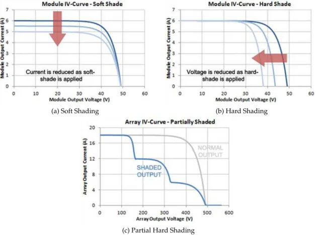
Through the analysis of the IV characteristics of a module, we can visualize how its output is affected by different types of shade. In the figure below 2.3, we can verify the effects on a IV curve of a system in case of soft, hard and partially hard shaded cells.
(a) Soft Shading (b) Hard Shading
(c) Partial Hard Shading
Figure 2.3: Effects on IV characteristic curves on solar systems taking into account the type of shade suffered. Source: Sargosis Solar & Electric, 2014.
Figure 2.3 summarises the impact of shading in the IV characteristics curve:
• IV Curve a) Soft Shade: Output voltage remains unaffected but less current will flow
from the module.
• IV Curve b) Hard Shade: Output current remains unaffected but the voltage
gener-ated by the module drops.
• IV Curve c) Partial Hard Shade (systems with at least two strings): a
If a system is working at its best performance, as the output voltage increases, the current of the module remains constant while the power is below the maximum power point. This point will be discussed later on. When reaching this point, the output current starts to drop. The way to verify this is by evaluating the IV curve sides, as these tend do get more sloped if the system is faulty. The measure of this effect is called the fill factor (Ff). It is calculated using the formula (2.1), shown below.
F f = Ipp·Vpp
Isc·Voc (2.1)
where:
Ipp is the peak power current (A)
Vpp is the peak power voltage (V)
Isc is the short circuit current, where the voltage is zero (A)
Voc is the open circuit voltage, where the current is zero (V)
If the fill factor is roughly below 70%, depending on the type of cells, this means there can be faulty modules or loose wires.
For every module, there is a point on its PV curve that is higher than any other point, at a specific voltage. This is called the Maximum Power Point3, which the solar inverter is designed to seek, in order to most effectively deliver the most power to the grid. However, the effects of shade cause this point to shift around as can be observed in figure 2.4.
Whenever shade is applied to a solar array, the inverter loses the ability to deliver the optimal amount of power, and must begin shifting its power-tracking point around, trying to find the new maximum. This behaviour on the part of the inverter can drastically reduce the power output of the array for a few minutes.
Figure 2.4 summarises the impact of shading in the PV characteristic curve4depicting the behaviour of the inverter tracking the MPP.
• PV Curve a) Soft Shade: The current drop induces a lower peak but maintaining a
similar shaped curve. tracking the new MPP is easy.
• PV Curve b) Hard Shade: The voltage drop induces a lower peak, but causing a
larger variation in the curve. Even though tracking the new MPP is not particularly difficult.
3Maximum Power Point (MPP), refers to the highest power output value the inverter can find in the PV
curve. The Maximum Power Point Tracking of a photovoltaic panel is performed in order to optimize its efficiency.
4PV Characteristic Curve, short for Power-Voltage Characteristic Curve, is a graphical curve which shows
(a) Soft Shading (b) Hard Shading
(c) Partial Hard Shading
Figure 2.4: Effects on PV characteristic curves on solar systems taking into account the type of shade suffered. Source: Sargosis Solar & Electric, 2014.
• PV Curve c) Partial Hard Shade: A shadow moving over the surface of several
modules over time has the effect of changing the PV curve from having a well defined maximum to a multi peaked shape. It is hard for the inverter to find the real MPP often setting for a lower power point.
2.2
Modelling Solar Systems
After seeing the importance of installations’ electric output prediction and the rele-vance of understanding its characteristics, this section details important aspects such as how a solar cell generates current and its mathematical model and equivalent circuit.
2.2.1 PN Juntion
P-type material. When a photon of light is absorbed by one of these atoms in the N-Type layer it will dislodge an electron, creating a free electron and a hole (Images SI Inc., 2007).
As this process happens, photons will create hole–electron pairs near the junction, causing the electric field in the depletion region to sweep holes into the P-side and sweep electrons into the N-side of the cell (Masters, 2004).
The process described above can be visualized in figure 2.5.
Figure 2.5: PN junction of a solar cell. Source: Masters, 2004.
If an external load is placed between the cathode (N-type silicon) to the anode (P-type silicon) electrons will be attracted to the positive charge of the P-type material travelling from the N-type material and back to the P-side creating a flow of electric current (Images SI Inc., 2007; Masters, 2004).
The hole created by the dislodged electron is attracted to the negative charge of N-type material and migrates to the back electrical contact. As the electron enters the P-type silicon from the back electrical contact it combines with the hole restoring the electrical neutrality (Images SI Inc., 2007).
The circuit described can be seen in figure 2.6.
Figure 2.6: Circuit linking a solar cell to a load. Source: Masters, 2004.
2.2.2 Mathematical Model and Equivalent Circuit of a PV Cell
2.7. The ideal current source delivers current in proportion to the solar flux to which it is exposed (Masters, 2004).
Figure 2.7: Equivalent circuit of a PV cell. Source: Masters, 2004.
There are several other models for the equivalent circuit of a solar cell as can been seen in figure 2.8, such as:
• Figure 2.8a) Ideal single diode model (ISDM), in which despite their simplicity, these
do not guarantee an accurate characteristic at the MPP.
• Figure 2.8b) Simplified single diode with a series resistance (SSDM).
• Figure 2.8c) Two-diode circuits are more accurate as they allows the system to keep
working under more cases than the other, accordingly the saturation current value of each diode.
(a) PV cell using the ideal
single-diode model. (b) PV cell using the Series resis-tance single-diode model. (c) PV cell circuit using one extradiode.
Figure 2.8: PV cell model examples drawn using a circuit simulator software.
The equivalent circuit of a PV cell is an adaptation to the single-diode model. It uses four components: photo-current source, diode parallel to source, series of resistorRS, and
shunt resistorRSH. This model is represented in figure 2.9 and is the most commonly used
model for conducting PV studies due to its accuracy (Krismadinata, Rahim, Ping, and Selvaraj, 2013).
Figure 2.9: Single-diode model - equivalent circuit of a PV cell. Source: Marnoto, Sopian, Daud, Algoul, and Zaharim, 2007.
where:
I is the output current (A)
IL is the photo-generated current (A)
ID is the diode current (A)
ISH is the shunt current (A)
RS is the series resistance (Ω)
RSH is the shunt resistance (Ω)
U is the voltage across the output terminals (V)
In this model, detailed below, the diode IV charactheristic is described through a non linear equation, which adds to its complexity (Drif, Pérez, Aguilera, and Aguilar, 2008).
Using Kirchoff’s Current Law (KCL), the current balance is given by equation 2.2.
I = IL−ID−ISH (2.2)
Considering the Shockley diode equation, the current diverted through the diode is given by equation 2.3.
ID = I0
enkTqUj −1
(2.3)
where:
Uj is the voltage across both diode and resistorRSHand it is given by:Uj =U+IRS(V)
Using the Ohm’s law, the current diverted through the shunt resistor is is given by equation 2.4.
ISH =
Uj
RSH
Substituting equations 2.3 and 2.4 into the first equation, the characteristic equation of a solar cell, which relates solar cell parameters to the output current and voltage, can be obtained. This means equation 2.2 can also be expressed as the equation 2.5.
I = IL−I0
emkTqUj −1
− Uj
RSH (2.5)
where:
I0 is the reverse saturation current (A)
q is the elementary charge carried by a single electron (q=1, 602×10−19C)
m is the diode ideality factor (m=1 for an ideal diode andm>1 for a real diode) k is the Boltzmann’s constant (k=1, 381×10−23J/K)
T is the absolute temperature (K)
Since the parametersI0,n,RS, andRSHcannot be measured directly, the best way to
tackle the characteristic equation of the PV cell is to apply a non-linear regression to extract the values of these parameters on the basis of their combined effect on the behaviour of the cell.
If the value of the shunt resistance RSH is much higher than the one of the series
resistance RS, then equation 2.5 can be simplified into the equation 2.9 shown below
(Marnoto, Sopian, Daud, Algoul, and Zaharim, 2007):
I = IL−I0
emkTqUj −1
(2.6)
Finally, using Kirchoff’s Voltage Law (KVL), the current balance is given by equation 2.7.
U=UD−RSI (2.7)
These expressions are extremely important for the work developed further on the thesis, specifically on the design of theoretical models on MATLAB5presented in in section 3.1 of chapter 3,Implementation.
There are two conditions of particular interest for the equivalent circuit of a PV cell. As shown in figure 2.10 those are:
5MATLAB is a high-level language for numerical computation, visualization, and application
• the current that flows when the terminals are short-circuited together, denominated
the short-circuit current,ISC;
• the voltage across the terminals when the leads are left open, denominated the
open-circuit voltage,UOC.
(a) Short-circuit current (ISC) (b) Open-circuit voltage (VOC)
Figure 2.10: Short-circuit current and open-circuit voltage. Source: Masters, 2004.
When the connections of the equivalent circuit for the PV cell are short-circuited together, as demonstrated in figure 2.10a, no current flows in the diode sinceU= 0, so all of the current from the ideal source flows through the short-circuited leads (Masters, 2004). It can be shown that for a high-quality solar cell (lowRSandI0, and highRSH) the
short-circuit currentISCis expressed by the equation 2.8.
ISC ≈ IL (2.8)
So it is possible to assume that:
I = ISC−I0
emkTqUj −1
(2.9)
Similarly, as demonstrated in figure 2.10b, when the cell is operated at open circuit, i.e., whenI =0, the voltage across the output terminals is defined as the open-circuit voltage. Assuming the shunt resistance is high enough to neglect the final term of the characteristic equation, the open-circuit voltageVOCis given by the following equation, equation 2.10:
VOC≈
mkT q ln
IL
I0
+1
(2.10)
It is not possible to extract any power from the device when operating at either open-circuit or short-open-circuit conditions.
In both these equations, the short-circuit current, ISC, is directly proportional to the
Figure 2.11: Photovoltaic IV relationship for "dark" (no sunlight) and "light" (illuminated cell). Source: Masters, 2004.
The dark curve is the curve of the diode shifted on the voltage axis. The light curve is the dark curve plusISC.
IV and PV characteristics of PV systems are popularly expressed in the form of IV curves that may be presented graphically or using non-linear equations (Marnoto, Sopian, Daud, Algoul, and Zaharim, 2007) as the output characteristics of a PV array vary non-linearly when temperature or irradiance conditions change (Kadri, Andrei, Gaubert, Ivanovici, Champenois, and Andrei, 2012).
2.3
Strategies to Optimize the Shading Effect on Solar Panels
2.3.1 Evolution in Optimization in the Past Decades
Complex designs and landscapes of PV systems usually necessary in urban environ-ments may provoke non-uniform operating conditions within the arrays resulting, as seen above, from factors such as varied panel orientation, presence of soiling or shading on the modules, or mismatched electrical characteristics between PV cells. Non-uniforme operating conditions cause module sections to sacrifice their individual power produc-tion potential, bringing the system to not operate at its maximum efficiency (MacAlpine, Erickson, and Brandemuehl, 2013).
Figure 2.12: Conventional grid-tie PV system with central inverter. Source: Tsao, 2010.
Next a few revolutionary technologies in the photovoltaic field and their contribution to minimize shading effects, are introduced further down:
• Micro-Inverters
• Power Optimizers
• Solar Tracking
• Solar Backtracking
Micro-Inverters
Micro-inverters are inverters which are installed on single solar modules. This tech-nology allows each module to independently generate AC current at its own optimal rate whether the other modules are shaded or not. The idea to design modules fitted with buit-in inverters, resulted from the conclusion that installation in domestic applications, even with string inverters, was not easy. This type of design was initiated in early 90’s under the name of OK4 and is also termed as Micro-Inverter (MI), Module Integrated Converters (MIC) or AC module (Sher and Addoweesh, 2012).
Although the initial idea of MI is not new, the latest developments in this field classify it as a new concept. With the use of a micro inverter each PV module produces its own AC power, therefore in case of failure of any individual module, power can still be supplied without any interruption (Canterbury Power Solutions, 2012). For example, in fig. 2.13 a case of partial shading affecting a module is depicted. In the case of a shunt connection (left), performance degradation due to shading, lowers the overall power output and the input voltage to the converter, if the connection is in shunt. Adverse situations like this can have less impact if micro-inverter technology is used (right).
Unfortunately, there are downsides to the micro-inverter approach (Canterbury Power Solutions, 2012; Sargosis Solar & Electric, 2014):
• lower efficiency of the micro-inverters compared to regular inverters, since they are
directly exposed to adverse environmental conditions like humidity, temperature, light etc.;
• reducing Mean Time to Failure (MTTF), and higher difficulty of repairing in cause
of faulty or malfunction
Figure 2.13: Micro-inverters application and power saving example. Source: Canterbury Power Solutions, 2012.
Power Optimizers
Although the discrete PV power generation solution provided by micro-inverters partially eliminates the shadow problem, its structure constrains the system energy har-vesting efficiency and entails high costs. The solar power optimizer was developed as an alternative to maximize the energy generated by each individual PV module. A power optimizer is a DC–DC converter with Maximum Power Point Tracking (MPPT), which increases PV panel voltage to optimum voltage levels for a DC microgrid connection or for a DC–AC inverter (Chen, Liang, and Hu, 2013).
There are many different system configurations in which distributed power electronics can be deployed accordingly to the mechanical orientation and electrical connection of the solar modules and to the power electronics devices in the system.
Figure 2.14 summarises the possible installations using power optimizers in conven-tional PV systems.
• PV Installation 2.14a) Power electronic devices installed on all the modules.
• PV Installation 2.14b) Power optimizers are installed in parallel output.
• PV Installation 2.14c) String optimizers are installed in parallel rows of panels.
(a) Distributed MPPT power opti-mizers on each module.
(b) Parallel output DMPPT power opti-mizers.
(c) String DMPPT power op-timizers.
Figure 2.14: Power optimizers installation examples. Source: Tsao, 2010.
of power optimizers allows the system to be designed in configurations that could not be used in conventional systems, offering options such as configurations with strings of different length connected using DMPPT6(MacAlpine, Erickson, and Brandemuehl, 2013; Tsao, 2010).
As with micro-inverters, power optimizers are an effective answer to the problems caused by shade, but their relative complexity raises their cost to a point that makes them economically unsuited most photovoltaic projects.
Solar Tracking
Even though a fixed flat-panel can be set to collect a high proportion of available noon-time energy, significant power is also available in the early mornings and late afternoons when the misalignment with a fixed panel becomes excessive to collect a reasonable proportion of the available energy. For example, even when the Sun is only 10◦
above the horizon the available energy can be around half the noon-time energy levels depending on latitude, season, and atmospheric conditions. Having this in consideration, a technology, known as solar tracking with the primary benefit of collecting solar energy for the longest period of the day, and with the most accurate alignment as the position of the sun, was developed .
Tracking systems are therefore responsible for orienting photovoltaic panels towards the sun, minimizing the angle of incidence to the incoming sunlight with the objective of increasing the amount of energy produced compared to a similar fixed installation (Lorenzo, Pérez, Ezpeleta, and Acedo, 2002). There are two possible installations, single or dual axis. According to the possible energy gain in each particular case, one of the two is used.
Single axis trackers have one degree of freedom that acts as an axis of rotation aligned along a true North meridian. There are several common implementations of single axis
6DMPPT, short for Distributed Maximum Power Point Tracker, is the technology of distributing the MPP
trackers, according to the orientation of the module, including: horizontal, horizontal with tilted modules, vertical, tilted and polar aligned.
Dual axis trackers, on the other hand, have two degrees of freedom that act as axes of rotation, which allows optimum solar energy levels due to their ability to follow the sun vertically and horizontally, the primary axis is fixed with respect to the ground and the secondary is typically perpendicular to primary. As happens with singles axis trackers, there are also several common implementations of dual axis trackers classified by the orientation of their primary axes to the ground such as: tip-tilt and azimuth-altitude. An example of this kind of installation is shown in figure 2.15.
Figure 2.15: Solar dual-axis tracker application example. Source: Queensland Windmill & Solar, 2008.
On clear sunny days the direct sunshine represents up to 90% of the total solar energy, with the other 10% from diffuse solar irradiance. However, on cloudy conditions, almost all of the solar irradiance is diffuse and identically distributed over the whole sky. Tests show that during overcast periods a horizontal module orientation increases the solar energy capture by nearly 50% compared to 2-axis solar tracking during the same period. This led to an improved of the tracking algorithm in which a solar array tracks the sun during cloud-free periods using 2-axis tracking, and switches to horizontal configuration case the sky becomes overcast (Kelly and Gibson, 2009) making this technology a good asset for solar energy harvesting on shading situations.
Solar Backtracking
When simple PV systems with more than one row of panels or arrays using single or dual axis solar tracker panels are receiving solar light at low angles, one panel may shade the panel behind it, rendering it less efficient, as can be seen in figure 2.16. This effect is more pronounced in winter when the solar angles are lower. A way of maximizing efficiency of the system in this cases is by the use of a technology called backtracking (Lauritzen Inc., 2011).
Figure 2.16: Example of installation without backtracking technology. Source: Sistemas Digitales de Control 2002, S.L., 2014.
As seen previously, shade reduces the electric output power and increases the risk of hot spots. Hence, the interest of the so called backtracking strategy as a mean of reducing shadowing impact (Lorenzo, Pérez, Ezpeleta, and Acedo, 2002). This is achieved by moving the surface angles away from then ideal values, just enough to get the shadow borderline to pass outside the border of the adjacent tracker. This way, first, shade is fully avoided and, second, the loss due to the angle of incidence is minimised (Lorenzo, Narvarte, and Muñoz, 2011). This is accomplished by flattening out the arrays in the morning and afternoon hours (i.e., zero tilt angle), using the precise control achievable with a microprocessor-based system (Panico, Garvison, Wenger, and Shugar, 1991).
The backtracking algorithm takes into account the topography of the site, position of the sun and the spacing, size and shape of the panels in the array to minimize shading and maximize orthogonality, so that the maximum amount of solar energy can be harvested (Lauritzen Inc., 2011). The system in figure 2.16 is re-shown in figure 2.17 illustrating the behaviour if backtrackers were installed.
Figure 2.17: Installation using backtracking technology. Source: Sistemas Digitales de Control 2002, S.L., 2014.
which offers benefits of flexibility, optimum fault tolerance, and cost savings associated with bypass and blocking diodes. The elimination of shading could result in increased system reliability via reduced reverse-bias conditions (Panico, Garvison, Wenger, and Shugar, 1991).
The use of backtracking can provide four main types of benefits:
Area-related benefits - Because backtracking systems permit smaller row-to-row spacing without penalty of shading, arrays can be closer-packed.
Performance-related benefits - Energy losses due to increased incidence angles, intro-duced by the elimination of inter-array shading, are lower than those resulting from shading. To this adds the fact that motor energy requirements are not relevant next to the gain of the system.
Reliability-related benefits - In addition to the benefits of reducing capital cost and enhancing energy production, backtracking can potentially improve PV installations reliability and variable operation and maintenance costs by significantly reducing the duration of reversed bias operating conditions in the array field.
Design-related benefits - The elimination of inter-array shadowing through backtracking allows systems to utilize series-configured panels. Tests showed that single series strings of cells with bypass diodes have the greatest fault tolerance to short circuit and open circuit component failures. The series string design provided the least life-cycle cost, based on repair and replacement of failed cells and modules.
The concept of backtracking was developed to lower balance of system costs, improve array performance, and increase long-term system reliability and has proven to be ex-tremely successful overcoming shading losses of conventional tracking and reducing the balance of system costs (Panico, Garvison, Wenger, and Shugar, 1991).
2.3.2 Use of Diodes to Compensate the Shading Effect on Solar Panels
Previously it was shown that diodes can be used to compensate the effect of shading on solar panels. In this section is described in detail how this process works.
As it is known, a diode is a semiconductor two-terminal device with the varying ability to conduct electrical current, i.e., to allow electrical current to pass in one direction but not the other.
In photovoltaic systems, there two types of diode installations used:
• Blocking Diodes
• Bypass Diodes
Figure 2.18: Bypass and blocking diode application. Source: Storr, 2014.
Blocking Diodes
Blocking diodes are usually connected at the end of a string or a series of panels and are used in photovoltaic installations equipped with batteries. These devices work as charge controllers, mainly to maintain isolation of power supplies, preventing reverse electrical currents from flowing back from the battery through the panels causing it do discharge (Prontes, 2013).
This type of diode assembly is also used as protective measure, protecting panels against other panels in cases of breakdown, ground fault issues and shading (Prontes, 2013).
Summarizing, blocking diodes are used in PV installations fitted with batteries isolating panel strings in order to prevent reverse currents from flowing through the panels in shading or other situations. (Prontes, 2013; Solar-Facts, 2012).
Bypass Diodes
Bypass diodes are connected in parallel with a string of panels or a single panel, providing an alternative current path around the cell block, if by chance, it becomes faulty or open-circuited due to overheating, per example. This prevents large voltages from building up across the solar cells in the reverse-biased direction, protecting the solar cells. (Deutsche Gesellschaft für Sonnenenergie, 2008; Sargosis Solar & Electric, 2014).
resistance. In these cases, the largest shading tolerance would be attained if bypass diodes were connected across every cell. In practice, however, bypass diodes are usually connected for manufacturing reasons across 18 to 20 solar cells. Consequently, modules with 36 to 40 cells have two bypass diodes, and modules with 72 solar cells have four bypass diodes (Deutsche Gesellschaft für Sonnenenergie, 2008). By creating an alternative current path through the shaded panel, bypass diodes also avoid wasting the power produced by the rest of the unshaded panels in the row (Sargosis Solar & Electric, 2014).
Since the diodes have a negligible voltage drop, the power loss induced by their presence is small. The only real loss from a shaded group of cells is whatever voltage they were providing (Sargosis Solar & Electric, 2014).
2.4
Methods for Calculating the Shade Factor for a Photovoltaic
System
The analysis of the various effects due to the presence of partial shading on PV systems is essential to avoid excessive power losses and to determine, for this cases, which is the best configuration to minimise adverse effects (Alonso-García, Ruiz, and Herrmann, 2006).
Considering the losses in performance provoked by the previously mentioned types of shading, the importance of taking shade effects into account and estimate them ahead is crucial as it can avoid unexpected results when setting up a photovoltaic system (Quaschning and Hanitsch, 1995).
In a PV system formed by several rows of panels, shading effects reduce the output energy essentially in three cases:
• Temporary shading;
• Shading due to the location;
• Shading cast by the building itself.
Temporary shading results from the presence of snow, fallen leaves in forested areas, bird droppings, and other types of dirt. For example, snow can be a significant factor for a system located at Serra da Estrela. The permanence of this dirt will be lesser as result of the self-cleaning of the system provided by the water of the rainfall (Greenpro, 2004; Karatepe, Boztepe, and Çolak, 2007).
Shading as a result of the location agglomerates all of the shading produced by sur-rounding high objects, including the neighbour buildings and trees which can possibly shade the photovoltaic system and/or at least darken of the horizon. The existence of cables above the building can also have a particularly negative effect, projecting shadows that are continuously moving (Greenpro, 2004).
structure, etc.. These shadows are constant therefore should be carefully considered when designing a photovoltaic installation, either trying to avoid them by moving the solar cells array or by moving the object that causes the shade. If none of these solutions are possible, the impact of the shading can be minimized in the system design phase, for example through the choice of how the cells and modules are interconnected (Greenpro, 2004).
Another degrading effect, apart from the three mentioned above, is concealing or masking the radiation from a panel row because of shade cast on it from the panel row in front. This is particularly serious if the distance between the rows is small, the position of the sun is low and the inclination is such that a large fraction of the total radiation is shaded possibly leading panel rows to become partly or even totally shaded by the previous rows (Passias and Källbäck, 1984).
These examples fortify the importance to have detailed knowledge of the system and its energy loss in order to determine its impact on the overall economy and performance of the installation.
The Shade Factor (SF) refers to the percentage of shade which the photovoltaic system is subjected to. The SF calculus assessment is intended to provide an indicative estimate of the potential shading on the solar array. This is done by indicating how much of the potential irradiance could be blocked by objects on the horizon at differing times of the day and of the year. This value can be calculated using numerical methods, either based only data obtained by observation or by computer means.
2.4.1 Calculations Based on Observation
One of the primordial stages in estimating irradiance on a shaded PV generator is conducting a survey of all objects/obstructions that can be found in its surroundings, such as: trees, buildings, etc. (Drif, Pérez, Aguilera, and Aguilar, 2008).
If there is an obvious clear horizon and no near or far shading, the assessment of SF can be considered non-existent and an SF value of 1 is assumed for all calculations. However, where there is a potential for shading, it should always be analysed and the reading should be taken from a location that represents the section of the array that is most potentially affected by shade. For systems with near shading in the northern hemisphere, this section will typically be just to the North of the near shading object ((MCS), 2012).
According to theGuide to the Installation of Photovoltaic Systems((MCS), 2012), one way to calculate the amount of potential irradiance that could be blocked by objects on the horizon at different times of the day and of the year, is to draw a sun path diagram with different arcs, each one referring to the months of the year, and lines for the time of the day resulting in a total of 84 segments each with an attributed value of 1%, used to produce a shading analysis for whichever objects in the horizon.
for the shading analyses respectively. It should be taken into account that the higher the number of segments, the best the accuracy estimating the Shade Factor.
To apply the method presented inGuide to the Installation of Photovoltaic Systemsthe observer has to stand as near as possible to the base and centre of the proposed array and face south, unless there is shading from objects within 10 m of distance ((MCS), 2012).
Once properly positioned, the observer should draw a line showing the uppermost edge of any objects that are visible on the horizon, either near or far, onto the sun path diagram. After the horizon line has been drawn, the number of segments that have been touched by the line, or that fall under the horizon line shall be counted. In figure 2.19 an example of this method is shown where is possible to see that there are 11 segments covered or touched by the horizon line ((MCS), 2012).
Figure 2.19: Sun path diagram of shading from objects over 10 m away. Source: (MCS), 2012.
The total number of segments is multiplied by their value(0, 01)and the total value shall be deducted from 1 to arrive at the shading factor. In the example in figure 2.19 the shading factor is calculated as follows.
SF determination for the example in figure 2.19:
1−(11×0, 01) =1−0, 11=0, 89
It is estimated that this shade assessment method will yield results within 10% of the actual annual energy yield for most systems. Unusual systems or environments may produce different results ((MCS), 2012).
The difference between considering the shade of objects further than 10 m away or within that distance is that the impact on system performance is higher at smaller distances from the array.
casting the shade should be relocated. If case this is not viable, the assessment of shading must be taken from a position more representative of the centre and base of the potentially affected array position.
As described previously, a standard horizon line shall be drawn to represent the worst case. This means the observer should stand on the array location most affected by shade. In addition, any objects on the horizon diagram, that are at 10 m or closer to any part of the array, shall have a shade circle added to the diagram to reflect the severe impact that these items may have on the array performance. Where there are multiple objects within 10 m, then multiple circles shall be drawn, one for each object ((MCS), 2012).
The shade circle shall have a radius equal to the height of the object and should be located so that the apex of the circle sits on the highest point of the shade object. All segments touched by, or within, the shade circle should be counted as part of the overall shade analysis ((MCS), 2012).
Figure 2.20: Sun path diagram of shading from objects within 10 m of distance from the away. Source: (MCS), 2012.
SF determination for the example in figure 2.20:
1−(40×0, 01) =1−0, 4=0, 6
value per section, it results in a shade factor of 0.6, as the calculus shows, compared with 0.89 obtained in the previous calculation.
2.4.2 Computer Aided Calculations and Software
More than a decade ago, budgeting, designing and planning of photovoltaic systems, was based on experience from past installations (Alonso-García, Ruiz, and Herrmann, 2006). Today it is possible to save time and money with the appropriate use of computer programs. System dimensioning and accurate enegy forecasts can be easily estimated in order to find the best choice from the energetic, economic and ecological point of view (Greenpro, 2004). Computer simulation is, therefore, a valuable tool since it makes it possible to model a great variety of situations impacting the performance of a system.
There is a wide range of software and simulation programs that can be used when planning a photovoltaic installation. These tools’ role is to assist with the design of photovoltaic systems by solving design problems and optimizing efficiency. A wide range of outputs can be generated by these programs, from the estimated produced energy, or theCO2emission reduction level to an economic viability analysis (Greenpro, 2004).
Sizing programs and simulators permit the estimation of threshold values and op-erating states,make possible the simulation of the operation in different conditions. In order to get accurate yield forecasts and yield reports, the use of simulators is mandatory. They have traditionally been employed in research and development, and component manufacturing.
In the process of improving, optimizing or developing new components and system concepts, simulation software is typically used. This helps reducing undesirable develop-ments and can also lessen the scope of experidevelop-ments. Furthermore these applications can also be put to good use for education and training purposes.
Usually, on simple programs, data parameters, meteorological data and its components, system surrounding details, and the intervention means, must be obtained from user descriptions and default tables (Greenpro, 2004).
As in most software applications, it must be noted that the greater the complexity and flexibility of a program, the higher the skills required from the user in order to take full advantage of its features (Deutsche Gesellschaft für Sonnenenergie, 2008; Greenpro, 2004).
Complex simulation programs, make possible to accelerate the planning process and avoid planning errors. However, they can create a lot of room for user mistakes, leading to unreliable results. The results of the simulation are only as good as the the quality of the inputs provided. Simulation results should be thought through critically and not blindly trusted (Deutsche Gesellschaft für Sonnenenergie, 2008).
PV software was divided into the following categories, according to their main pur-poses:
Simulation Tools - Energy simulation programs which provide functions that can be linked to concrete solutions such as simulating meteorological data, electrical and thermal energy components etc.
Economic Evaluation Tools - Performance and economic model software, designed to facilitate decision making for the photovoltaic energy investment community.
Photovoltaic Industry Related Tools - Software tools for every manufacturing step of PV installations. This kind of tool includes analysing experimental data, calculating optimum architecture based on specific materials, and even research assistant tools. Using PV industry related tools suppliers can simulate their new products and measure the impact of design decisions in a virtual process flow.
Analysis, Design and Planning Tools - PV software calculator of potential electricity production. These tools can compare PV output on the basis of different technology options such as module type, inverter efficiency, and mounting type. They may also contain an interactive horizon editor for the purpose of shading analysis.
Monitoring and Control Tools - Satellite based tool for local and/or remote monitoring of photovoltaic systems which use solar and meteo data. They feature new gener-ation software to calculate the expected energy yield of PV systems,without the need to rely on data loggers or ground sensors. Hence, the calculated yield is not influenced by faulty or ill maintained sensors.
Site Analysis Tools - Range of analysis programs that allow designers to work in 3D with an advanced parametric CAD tool. These standardization tools also provide developers and designers access to a comprehensive. One additional feature typically present is the ability to calculate shadows on arbitrarily oriented surfaces.
Solar Radiation Maps - Tools that provide geographical assessment of solar resource and performance, based upon satellite earth observations. They were introduced in order to allow a worldwide study of how much energy is provided by the sun under different weather conditions.
Following the trend of the software industry, a number of Smart Phone Apps became available. Those typically allow users to make measurements, check solar irradiation and potential shading. They can be useful when projecting a new installation in situations where access to a more comprehensive software is not available.
Concluding, it can be said that currently there is a widespread availability of mature, sophisticated tools that can be used in any phase of photovoltaic system deployment, from the business plan to the monitoring tasks.
The following table (table 2.1) lits existing software applications according to their category:
Table 2.1: Examples of photovoltaic software per category.
Photovoltaic Software Categories
Categories Software Examples
Simulation
INSEL
TRaNsient SYstem Simulation Program (TRNSYS) DASTPVPS SOLinvest Pro PVsim SITOP Solar Pro Economic Evaluation HOMER
Solar Advisor Model (SAM) RETScreen
SOLinvest EnergyPeriscope PVWatts Calculator
PV Industry Related
APOS photovoltaic StatLab
Organic Photovoltaics Analysis Platform PV Cost Simulation Tool
Analysis, Design and Planning
pvPlanner Archelios PRO String Design Tool PVSYST PV*Sol Solarius-PV PV F-CHART PV DesingPro Greenius SUNDI PVCad
Monitoring and Control
Continuation of Table 2.1
Categories Software Examples
Site Analysis
Autodesk ECOTECT Analysis Shadow Analyzer
Shadows MeteoNorm
Amethyst ShadowFX Horizon
Skelion
Solar Radiation Maps
Photovoltaic Geographical Information System (PVGIS) Focus Solar
SolarGIS
White Box Technologies
Available Mobile apps (smartphone/PDA) include EasySolar, Scan The Sun and Pyrom-eter. Examples of Cloud Based tools include SolarDesignTool, PVAnalytics and modsolar.
2.4.3 Shading Simulation Software Review
In this subsection, a review of the software used for dealing with or avoiding the various shading effects is made.
As previously discussed, shading situations present a particular challenge in the planning process. The following aspects have to be considered: shading occurrence at many sites for PV systems, module rows shading each other, edge shading or elevated horizons, the environment, among others. Shading has an effect on the system yield and should be considered on optimised system design (where bypass and blocking diodes, module wiring and inverter behaviour are considered). Simulation programs are therefore essential for calculating shading losses and optimising the electrical and geometric system design (Deutsche Gesellschaft für Sonnenenergie, 2008).
On basic applications, the losses due to shading are estimated by the user and may, therefore, be detached from reality. Since shading calculations based mainly on observation and set by a common user have a relatively high rate of error, vendors of sophisticated applications invested in the modelling of shading behaviour and developed algorithms to estimate its effects on the system performance.
Below, in table 2.2 are identified the most popular products and their features:
pvPlanner Shadow Analyzer
Shadows ShadowFX PVCad PVSYST PV*Sol Archelios PRO Project Location with Google Maps ✔ ✖ ✖ ✔ ✖ ✖ ✖ ✔ World wide Meteo Database ✔ ✖ ✔ ✔ ✔ ✔ ✔ ✔ PV Devices
Database ✔ ✖ ✖ ✖ ✔ ✔ ✔ ✔
Sunpath
Diagrams ✔ ✔ ✔ ✔ ✔ ✖ ✖ ✔
3D Solar
Models ✖ ✔ ✖ ✔ ✔ ✔ ✔ ✔
Solar
Reports ✔ ✔ ✔ ✔ ✔ ✔ ✔ ✔
Economics
Results ✔ ✖ ✖ ✖ ✔ ✔ ✔ ✔
Table 2.2: Shading software chart.
Most of the software mentioned in table 2.2 has a whole range of other less meaningful features, besides its 3D shading calculations tool, such as the ability to import system mea-surement data for directly comparing measured and simulated values, and the availability toolboxes for solar geometry, meteorology and photovoltaic operational behaviour.
Programs, likePVSYS,Archelios PROandPVCadalso allow special analysis, such as the calculation of module characteristic curves in partial shading situations, enabling, for example, the determination of the thermal loading on solar modules. Moreover, it is possible to produce outputs containing all sorts of parameters, such as meteorological data, electrical voltages, currents, energies and performances (Deutsche Gesellschaft für Sonnenenergie, 2008; Greenpro, 2004).
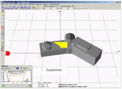
Snaps of PVSYST and PVCad are shown in figures 2.21 and 2.22.
Figure 2.21: 3D editing tool on PVSYST. Source:Solar PV System Shading Calculation with PVSYST - YouTube
2009.
Figure 2.22: Module positioning analysis on PVCad. Source:Controlling software for photovoltaics - PVCAD
2015.
of photovoltaic systems. Its shading analysis undergoes automatic calculation of distant shadows and the shading factor. It has the capability of importing data from different sources such as7PVGIS shading data, 3D Google SketchUp files for near shading factor calculation and Solmetric SunEye shade measurements. Archelios also integrates with
7PVGIS, short for Photovoltaic Geographical Information System, is a solar radiation database, built