Capture of pollutants from post-combustion streams with ionic liquids

I

Luís Manuel

Cravo Pereira

Captura de Poluentes de Correntes Pós-combustão

com Líquidos Iónicos

Capture of Pollutants from Post-combustion

Streams with Ionic Liquids

III

Luís Manuel

Cravo Pereira

Captura de Poluentes de Correntes Pós-combustão

com Líquidos Iónicos

Capture of Pollutants from Post-combustion

Streams with Ionic Liquids

Dissertação apresentada à Universidade de Aveiro para cumprimento dos requisitos necessários à obtenção do grau de Mestre em Engenharia Química, realizada sob a orientação científica do Dr. João Manuel da Costa e Araújo Pereira Coutinho, Professor Associado com Agregação do Departamento de Química da Universidade de Aveiro, e co-orientação da Dra. Mariana Belo Oliveira, Estagiária de Pós-doutoramento do Departamento de Química da Universidade de Aveiro.

V Dedico este trabalho aos meus pais e irmãos.

VII

o júri

presidente Prof. Doutor Carlos Manuel Santos Silva

Professor Auxiliar do Departamento de Química da Universidade de Aveiro

Prof. Doutor João Manuel da Costa e Araújo Pereira Coutinho

Professor Associado com Agregação do Departamento de Química da Universidade de Aveiro

Doutora Mariana Belo Oliveira

Estagiária de Pós-Doutoramento no Departamento de Química da Universidade de Aveiro

Doutora Ana Maria Antunes Dias

Estagiária de Pós-Doutoramento no Departamento de Química da Faculdade de Ciências e Tecnologia da Universidade de Coimbra

IX

agradecimentos

Em primeiro lugar gostaria de agradecer ao Prof. João Coutinho pela possibilidade de ter realizado a minha tese mestrado sob a sua orientação. Os seus conselhos, perseverança e carácter único contribuíram não só para a realização de um melhor trabalho, mas sobretudo para a minha formação como pessoa e investigador.

Não posso também esquecer a excelente orientação do Pedro Carvalho. A sua extensa experiência nos mais diversos temas, o seu amplo conhecimento nas diferentes técnicas aplicadas neste trabalho e uma personalidade inigualável tornaram este percurso muito mais enriquecedor. A ele, o meu muito obrigado!

Gostaria também de agradecer à Ana Dias, à Mariana Belo e ao Fèlix Llovel pela disponibilidade, ajuda e conhecimentos transmitidos durante a modelação dos sistemas.

Nunca esquecerei os momentos que só um grupo como o Path poderia ter proporcionado. Sem nunca esquecer ninguém, gostaria de agradecer à Marta Batista, à Sónia Ventura e ao Jorge Pereira pelos seus conselhos e ocasiões de descontração, muito importantes para uma investigação saudável. Gostaria de agradecer em especial também ao Félix Carreira, companheiro para a vida, pelo seu apoio e sugestões que tanto ajudaram a ultrapassar obstáculos.

Por fim, e por isso não menos importante, gostaria de agradecer aos meus pais, irmãos e a Margarida Cabral pelo infinito e incondicional apoio que me deram durante este curso. Isto é para vocês!

XI

palavras-chave Líquidos iónicos, solubilidade de gases, dióxido de carbono, azoto, óxido

nitroso, metano, soft-SAFT EoS, seletividades.

resumo O aumento da emissão de poluentes nitrogenados, bem como as

limitações presentes nos atuais métodos de controlo e o aparecimento de novas legislações e limites máximos de emissão, requerem o desenvolvimento de novos métodos para a redução destes poluentes.

Os Líquidos Iónicos (LIs), pelas suas características únicas e baixa pressão de vapor, têm despertado uma grande atenção durante a última década e estão a tornar-se numa nova classe de solventes muito promissores para a captura de poluentes e separação de gases, quer como fase estacionária num processo de membranas quer como absorvente num processo de extração. Não obstante, o desenvolvimento de novos processos de controlo, ou melhoria dos já existentes, requerem o conhecimento do equilíbrio gás-líquido (EGL) que é, até ao momento, ainda insuficiente.

Neste trabalho, a solubilidade de gases presentes em processos de combustão como o azoto (N2), o metano (CH4), óxido nitroso (N2O) e dióxido

de carbono (CO2) num líquido iónico muito polar foram estudados através de

medições do EGL. Os resultados demostram a já reconhecida elevada solubilidade de N2O e CO2 em LIs bem como a elevada seletividade em

relação ao ar devido à baixa solubilidade do N2 nos LIs. Foi ainda observado

que, contrariamente aos outros gases, para os sistemas N2 + LIs o aumento da

temperatura provoca uma aumento da solubilidade do gás.

A descrição dos sistemas anteriores por modelos teóricos é fundamental para o projeto de potenciais técnicas de redução de poluentes. Neste sentido, a soft-SAFT EoS, que tem demonstrado ser capaz de descrever sistemas com LIs com enorme sucesso, foi usada para descrever os diferentes sistemas publicados na literatura e medidos aqui em função da temperatura, composição e pressão, permitindo deste modo estender a aplicabilidade do modelo a novos sistemas. Novos parâmetros moleculares, necessários para a descrição de cada componente, são propostos neste trabalho para o N2O e

para três dos cinco LIs estudados. Os resultados demonstraram uma boa descrição dos dados experimentais, tanto no que diz respeito ao comportamento inverso observado para o N2 como a baixa dependência do

CH4 com a temperatura.

Finalmente, a capacidade de extração dos LIs bem como a sua seletividade é comparada com a dos solventes utilizados nos métodos de controlo atuais, como monoetanolamina (MEA) e éter monometílico de trietilenoglicol (TEGMME). Os resultados demonstram uma capacidade de extração dos LIs igual ou superior à dos solventes convencionais, aliada a uma elevada seletividade em relação ao N2O e CO2.

Com base neste trabalho, pode-se afirmar que os LIs, devido às suas características únicas e elevada seletividade, apresentam um grande potencial para serem utilizados na captura de poluentes.

XIII

keywords Ionic liquids, gas solubilities, carbon dioxide, nitrogen, nitrous oxide, methane,

soft-SAFT EoS, seletivities.

abstract The increase in nitrogenated pollutants emissions, along with the

limitations of the existing control methods and future stricter legislation, demands the development of new methods to reduce such pollutants.

Ionic liquids (ILs), due to their unique characteristics and low vapour pressure, have attracted a large attention during the last decade and are becoming a promising class of solvents to capture pollutants and for gas separation, either as a stationary phase in a membrane process or as an absorption solvent in an extraction process. Nonetheless, the development and/or improvement of new/existing control processes requires the knowledge of gas-liquid equilibrium (GLE) data for ILs + gas systems that are, at the moment, still scarce.

The solubilities of some common gases present in combustion processes, such as nitrogen (N2), methane (CH4), nitrous oxide (N2O) and carbon dioxide

(CO2), were studied through the experimental measurement of the GLE. The

results showed a high solubility of N2O and CO2 compared to N2. Furthermore,

a surprisingly increase of the solubility of N2 with temperature was observed.

The description of previous systems by theoretical models stands also as a vital task for the development of techniques to reduce pollutants. In this sense, the soft-SAFT EoS has proven to be able to describe systems with ILs with a huge success and in a predictive manner. Thus, this model was used to describe the GLE data available in the literature and measured here, for different temperatures and for all concentrations and pressures ranges studied, in order to extend the applicability of the soft-SAFT EoS to describe/predict the gas + ILs systems. The molecular parameters necessary for the description of each compound were determined for the first time in this work for N2O and

three of the five ILs involved. The results showed a good description of the experimental data. In addition to that, soft-SAFT EoS successfully predicts the peculiar behaviour observed for N2 as well as the low temperature dependence

observed for the CH4 systems.

Finally, the extraction capacity and gases selectivity in the ILs was compared with other solvents used in the reduction of pollutants, such as monoethanolamine (MEA) and triethylene glycol monomethyl ether (TEGMME). The results showed a similar or higher extraction capacity of the ILs compared to conventional solvents, combined with a high selectivity towards N2O and

CO2.

Based on the results showed on this work, it is suggested that ILs due to their unique characteristics and high selectivity are promising agents to capture pollutants.

XV

List of Contents

List of Figures ... XVII List of Tables ... XX Nomenclature ... XX List of Symbols ... XXI List of Abbreviations ... XXI Superscripts... XXIII Subscripts ... XXIII

1- General Introduction ... 1

1.1- Scope and Objectives ... 3

1.2- Air Pollution ... 4

1.3- Nitrogenated Compounds ... 7

1.4- Control Methods for Nitrogenated Compounds ... 9

1.5- Control Methods Insufficiency... 12

1.6- Ionic Liquids ... 13

1.7- Soft-SAFT EoS ... 15

2- Molecular Models ... 19

2.1- Introduction ... 21

2.2- ILs Molecular Parameters ... 21

2.3- Gases Molecular Parameters ... 26

3- Gas Solubilities ... 31

3.1- Introduction ... 33

3.2- Materials and Experimental Equipment ... 33

3.2.1- Materials ... 33

3.2.2- Experimental Equipment ... 34

3.3- Experimental Results and Soft-SAFT EoS Modelling. ... 36

3.3.1- CO2 Solubility ... 36

3.3.2- N2O Solubility ... 37

3.3.3- CH4 Solubility ... 38

3.3.4- N2 Solubility ... 40

3.4- Extension of Soft-SAFT Modelling to Other ILs + Gas Systems ... 42

3.4.1- CO2 Solubility in Other ILs ... 42

3.4.2- N2O Solubility in Other ILs ... 44

3.4.3- N2 Solubility in Other ILs ... 47

4- ILs’ Capturing Efficiency and Selectivities ... 49

4.1- Introduction ... 51

4.2- Henry’s Constants and Selectivities ... 52

4.3- ILs’ Capturing Efficiency ... 54

5- Conclusions ... 57

6- Future Work ... 61

7- References ... 65

XVI

Parameters ... 81

Appendix D- Solubility of CO2 and N2O in TEGMME ... 86

Appendix E- Henry’s Constant Calculation ... 87

XVII

List of Figures

Figure 1.1- Composition (% v/v) of Earth's Atmosphere, adapted from Jacob et al.30 ... 5

Figure 1.2- Evolution of NOx emissions by source sector in the EU adapted from the 2011 Air Quality report44 (1 Gg=1000 tonnes/year). ... 8

Figure 1.3- Total annual anthropogenic N2O emission in the UE (average 1990-1998), adapted from Pérez-Ramírez et al.46 ... 8

Figure 1.4- Evolution of the atmospheric N2O concentration, adapted from Pérez-Ramirez et al.46 9 Figure 1.5- US primary energy consumption forecast till the year 2035 adapted from the Annual Energy Outlook 2012.48 ... 12

Figure 1.6- Cations and anions commonly used to form ILs. ... 13

Figure 1.7- Molecule model within the soft-SAFT approach. ... 16

Figure 2.1- Proposed association scheme for [C4mim][BF4] by Andreu et al.22 ... 22

Figure 2.2- Proposed association scheme for [C4mim][NTf2] by Andreu et al.23 ... 22

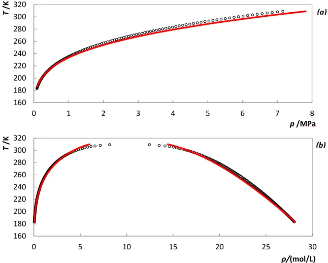
Figure 2.3- [C4mim][BF4] (a) and [C4mim][NTf2] (b) temperature-density diagrams.117, 118 Solid lines represent soft-SAFT EoS predictions. ... 23

Figure 2.4- Scheme of association adopted in this work for the ILs [C4mim][SCN] (a), [C2mim][CH3OHPO2] (b) and [C4mim][N(CN)2] (c). ... 23

Figure 2.5- Temperature-density diagram for [C4mim][SCN].54 Solid lines represent soft-SAFT EoS predictions with a limit temperature of application of 290.05 K. ... 25

Figure 2.6- Temperature-density diagram for [C2mim][CH3OHPO2].121 Solid lines represent soft-SAFT EoS predictions with a limit temperature of application of 290.05 K. ... 25

Figure 2.7- Temperature-density diagram for [C4mim][N(CN)2].122 Solid lines represent soft-SAFT EoS predictions with a limit temperature of application of 288.40 K. ... 25

Figure 2.8- CH4 temperature-pressure (a), CH4 temperature-density (b), CO2 temperature-pressure (c), CO2 temperature-density (d), N2 temperature-pressure (e) and N2 temperature-density (f) diagrams. Experimental data was taken from NIST database.124 Solid lines represent the soft-SAFT EoS predictions. ... 27

Figure 2.9- N2O molecular structure. ... 28

Figure 2.10- px diagrams for N2O in the ILs [C4mim][BF4]16 (a) and [C4mim][NTf2]18 (b) at 323 K. Solid lines represent soft-SAFT EoS predictions at 323 K using the different sets of parameters for N2O listed in Table 2.4 and both binary parameters fixed to 1... 29

Figure 2.11- Temperature-pressure (a) and temperature-density (b) diagrams for N2O taken from NIST database.124 Solid lines represent soft-SAFT EoS prediction using the parameters set 4 for N2O. ... 30

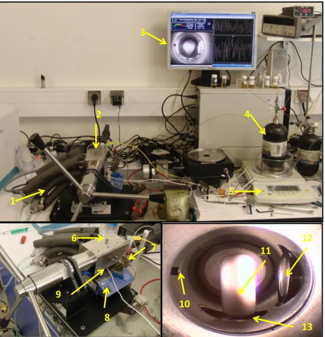
Figure 3.1- Components of the high pressure cell: 1) Thermostatized bath circulator; 2) High pressure cell; 3) Video and data acquisition; 4) Gas storage; 5) Analytical balance; 6) Temperature sensor; 7) Valves; 8) Magnetic stirrer; 9) Piezoresistive pressure transducer; 10) Gas entrance; 11) Magnetic bar; 12) Light source from an optical fiber cable; 13) Pressure probe. ... 34

XVIII

Figure 3.3- px diagram for the system N2O + [C2mim][CH3OHPO2] at different temperatures. Solid lines represent soft-SAFT EoS predictions using one temperature independent and non-dependent binary parameter ( ). ... 37 Figure 3.4- Binary parameters ( ) used for describing the system N2O + [C2mim][CH3OHPO2]... 38 Figure 3.5- px diagram for the system CH4 + [C2mim][CH3OHPO2] at different temperatures. Solid lines represent soft-SAFT EoS predictions using one temperature dependent binary parameters ( ). ... 38 Figure 3.6- pT diagram for the system CH4 + [C2mim][CH3OHPO2] at different gas composition. Solid lines represent soft-SAFT EoS predictions using one temperature dependent binary parameters ( ). ... 39 Figure 3.7- Binary parameters ( ) used for describing the system CH4 + [C2mim][CH3OHPO2]. ... 39 Figure 3.8- px (a) and pT (b) diagrams for the system N2 + [C2mim][CH3OHPO2]. Solid lines represent soft-SAFT EoS predictions with one temperature dependent and independent binary parameters ( ). ... 41 Figure 3.9- Binary parameters ( ) used for describing the system N2 + [C2mim][CH3OHPO2]. ... 41 Figure 3.10- px diagram for the system CO2 + [C4mim][SCN] at different temperatures.15 Solid lines represent soft-SAFT EoS predictions using one temperature independent binary parameter ( =0.965). ... 42 Figure 3.11- px diagram for the system CO2 + [C4mim][BF4] at different temperatures.17 Solid lines represent soft-SAFT EoS predictions using both binary parameters ( and ) fixed to 1. ... 42 Figure 3.12- px diagram for the system CO2 + [C4mim][NTf2] at different temperatures.19 Solid lines represent soft-SAFT EoS predictions using one temperature independent binary parameter ( =0.98). ... 43 Figure 3.13- px diagram for the system CO2 + [C4mim][N(CN)2] at different temperatures.20 Solid lines represent soft-SAFT EoS predictions using one temperature independent binary parameter ( =0.89). ... 43 Figure 3.14- px diagram for the system N2O + [C4mim][N(CN)2] at different temperatures. Solid lines represent soft-SAFT EoS predictions using one temperature independent parameter ( =0.915). ... 44 Figure 3.15- px diagram for the system N2O + [C4mim][SCN] at different temperatures.14 Solid lines represent soft-SAFT EoS predictions using one temperature independent binary parameter ( =0.978). ... 45 Figure 3.16- px diagram for the system N2O + [C4mim][BF4] at different temperatures.16 Solid lines represent soft-SAFT EoS predictions using one temperature independent binary parameter ( =0.978). ... 45 Figure 3.17- px diagram for the system N2O + [C4mim][NTf2] at different temperatures.18 Solid lines represent soft-SAFT EoS predictions using two temperature independent binary parameters ( =1.01 and =0.98). ... 46

XIX Figure 3.18- px (a) and pT (b) diagrams for the system N2 + [C4mim][N(CN)2. Solid lines represent soft-SAFT EoS predictions using one temperature dependent and independent binary parameters ( ). ... 47 Figure 3.19- Binary parameters ( ) used for describing the system N2 + [C4mim][N(CN)2]. ... 48 Figure 4.1- MEA (a) and TEGMME (b) molecular structures. ... 51 Figure 4.2- Predicted solubility of N2 in TEGMME at 303 K using PSRK EoS and adjusted polynomial function. ... 52 Figure 4.3- Calculated in the different solvents within the temperature range of (298.15–303.38) K. ... 53 Figure 4.4- Calculated (blue) and (red) in the different solvents within the temperature range of (298.15–303.38) K. ... 53 Figure 4.5- pmg/s diagram of N2O in different solvents within the temperature range of (298.10–

303.31) K. Solid lines are only used as guide lines. ... 54 Figure 4.6- pmg/s diagram of CO2 in different solvents within the temperature range of (298.11–

303.22) K. Solid lines are only used as guide lines. ... 55 Figure 8.1- Diagram of the Atmospheric nitrogen cycle, adapted from Seinfeld et al.1 ... 79 Figure 8.2- px diagrams for the systems CO2 (a) and N2O (b) in TEGMME at 303 K. Solid lines represent PSRK EoS predictions obtained with a commercial simulator (ASPEN Plus 2006.5). N2O solubility data was taken from the literature,146 while for CO2 experimental points were calculated through the Henry’s constant reported in Henni et al. work’s.147 ... 86 Figure 8.3- px diagram for the system CO2 + [C2mim][CH3OHPO2] at different temperatures. Solid lines represent soft-SAFT EoS prediction adjusted for the lowest gas composition using specifics binary parameters ( ). ... 87 Figure 8.4- px diagram for the system N2O + [C2mim][CH3OHPO2] at different temperatures. Solid lines represent soft-SAFT EoS prediction adjusted for the lowest gas composition using specifics binary parameters ( ). ... 88 Figure 8.5- px diagram for the system N2 + [C2mim][CH3OHPO2] at different temperatures. Solid lines represent soft-SAFT EoS prediction adjusted for the lowest gas composition using specifics binary parameters ( ). ... 89 Figure 8.6- px diagram for the system N2 + [C4mim][N(CN)2] at different temperatures. Solid lines represent soft-SAFT EoS prediction adjusted for the lowest gas composition using specifics binary parameters ( ). ... 90

XX

Seinfeld et al. ... 5

Table 1.2- Estimate of Global Tropospheric NOx emission in the year 2000, adapted from Seinfeld et al.1 (1 Tg nitrogen=1012 g nitrogen). ... 7

Table 1.3- Summary of NOx removal efficiency reported in the literature for diverse techniques. 10 Table 2.1- Molecular parameters for [C4mim][BF4]and [C4mim][NTf2] taken from the literature.22, 24 ... 22

Table 2.2- Adjusted molecular parameters for [C4mim][SCN], [C4mim][N(CN)2] and [C2mim][CH3OHPO2]. ... 24

Table 2.3- Soft-SAFT molecular parameters for CH4, CO2 and N2 taken from the literature.12, 26, 27 26 Table 2.4- Set of adjusted molecular parameters for N2O. ... 28

Table 4.1- Gases Henry’s constants in the ILs within the temperature range of (298.15–303.38) K. ... 53

Table 4.2- N2O and CO2 solubility expressed in terms of molar fraction and molality within a temperature range of (298.10–303.31) K and a pressure of 2 MPa. ... 55

Table 8.1- Full list of adjusted molecular parameters for N2O... 80

Table 8.2- Bubble point data and IL and gas mass of the system CO2 + [C2mim][CH3OHPO2]. ... 81

Table 8.3- Bubble point data and IL and gas mass of the system N2O + [C2mim][CH3OHPO2]. ... 82

Table 8.4- Soft-SAFT Eos temperature dependent binary parameters ( ) used for the system N2O + [C2mim][CH3OHPO2] at average temperatures (Ta)... 83

Table 8.5- Bubble point data and IL and gas mass of the system CH4 + [C2mim][CH3OHPO2]. ... 83

Table 8.6- Soft-SAFT Eos temperature dependent binary parameters ( ) used for the system CH4 + [C2mim][CH3OHPO2] at average temperatures (Ta)... 84

Table 8.7- Bubble point data and IL and gas mass of the system N2 + [C2mim][CH3OHPO2]. ... 84

Table 8.8- Soft-SAFT Eos temperature dependent binary parameters ( ) used for the system N2 + [C2mim][CH3OHPO2] and N2 + [C4mim][N(CN)2] at average temperatures (Ta). ... 85

Table 8.9- Calculated Henry’s constants of CO2 in [C2mim][CH3OHPO2] at different temperatures, minimum square error (R2) obtained in the linear regression adjusted for a gas composition up to 0.05 and binary parameters ( ) used in the soft-SAFT EoS predictions. ... 87

Table 8.10- Calculated Henry’s constants of N2O in [C2mim][CH3OHPO2] at different temperatures, minimum square error (R2) obtained in the linear regression adjusted for a gas composition up to 0.05 and binary parameters ( ) used in the soft-SAFT EoS predictions. ... 88

Table 8.11- Calculated Henry’s constants of N2 in [C2mim][CH3OHPO2] at different temperatures, minimum square error (R2) obtained in the linear regression adjusted for a gas composition up to 0.01 and binary parameters ( ) used in the soft-SAFT EoS predictions. ... 89

Table 8.12- Calculated Henry’s constants of N2 in [C4mim][N(CN)2] at different temperatures, minimum square error (R2) obtained in the linear regression adjusted for a gas composition up to 0.02 and binary parameters ( ) used in the soft-SAFT EoS predictions. ... 90

XXI

Nomenclature

List of Symbols

Helmholtz energy f Function (Chapter 1) f Fugacity (Chapter 4)

gLJ Radial distribution function of a fluid of LJ spheres

kB Boltzman’s constant

kHB Association site volume

m Number of segments

M Number of association sites

mg/s Molality mi Mass of component i N Number of points p Pressure Q Quadrupole T Temperature

xi Molar fraction of the component i

xp Fraction of the chain with the quadrupole

Z Studied property

ε/kB Dispersive energy between segments forming the chain

εHB/kB Association site energy

μ Chemical potential

ρ Density

σ Segment size

Binary parameter for correcting deviations in the molecular size Binary parameter for correcting deviations in the molecular energy

List of Abbreviations

%AAD Percentage average absolute deviation

[C2mim][CH3OHPO2] 1-ethyl-3-mthylimidazolium methylphosphonate [C4mim][BF4] 1-butyl-3-methylimidazolium tetrafluoroborate [C4mim][N(CN)2] 1-butyl-3-methylimidazolium dicyanamide

XXII

Ar Argon

BOOS Burners Out of Service

BSI BioSolids Injection

C2F6 Perfluoroethane

CAA Clean Air Act

CF4 Perfluoromethane

CH4 Methane

CO Carbon monoxide

CO2 Carbon dioxide

EPA Environmental Protection Agency

EU European Union

GLE Gas-liquid equilibrium

GWP Global Warming Potential

H Henry’s constant

H2O Water

H2S Hydrogen sulphide

HFC-23 Fluoroform

HNO3 Nitric acid

IL Ionic liquid

ILs Ionic liquids

LJ Lennard-jones

LNB Low-NOx Burner

LTOA Low-Temperature Oxidation with Absorption

MEA Monoethanolamine

N2 Nitrogen

N2O Nitrous oxide

N2O4 Dinitrogen tetroxide

N2O5 Dinitrogen pentoxide

NH3 Ammonia

NO Nitrogen monoxide

XXIII

NOx Oxides of nitrogen

O2 Oxygen

O3 Ozone

OFA Over Fire Air

Pb Lead

PM Particulate matter

S1/2 Ideal selectivity between the gases (1 and 2) in a specified solvent

SAFT Statistical Associating Fluid Theory

SCR Selective Catalytic Reduction

SH6 Sulphur hexafluoride

SNCR Selective Non-catalytic Reduction

SO2 Sulphur dioxide

Soft-SAFT EoS “Soft” statistical associating fluid theory equation of state TEGMME Triethylene glycol monomethyl ether

TPT1 Wertheim’s first-order thermodynamic perturbation theory

US United States

vdW-1f Van der Waals one-fluid theory

VOCs Volatile Organic Compounds

WHO World Health Organization

Superscripts

assoc Association interactions term

chain Chain term

polar Polar interactions term

res Reference term

Subscripts

i Component i

liq Liquid phase

XXV

“The satisfaction and good fortune of the scientist lies not in the peace of possessing knowledge but in the toil of continually increasing it.”

1

3

1.1- Scope and Objectives

The increase of pollutants emissions along with the limitations presented by the existing control methods and stricter legislation to come, demands the investigation of new methods and ways to reduce some pollutant levels. This is particularly important for nitrogenated compounds, such as oxides of nitrogen (NOx) and nitrous oxide (N2O), whose emissions increase has an important effect on the atmosphere and human health.1

Ionic liquids (ILs) have attracted an outstanding attention during the last decade and are turning to be a promising class of solvents in the capture pollutants and also in gas separations due to their unique characteristics and low vapour pressure. Therefore, the possibility of using ILs as capturing agents for nitrogenated compounds is here evaluated and discussed by studying the gas-liquid equilibrium (GLE) of N2O in several ILs. N2O was here chosen as a representative molecule for the nitrogenated compounds due to its low adverse effects on human health when compared to NOx.2 Nitrogen (N2) and carbon dioxide (CO2), the major constituents of post-combustion streams,3 and methane (CH4), produced in higher concentration, for instance, during the incomplete combustion or at low temperatures combustion of natural gas streams,4 are also investigated through the study of their GLE in the ionic liquid (IL), aiming at understanding ILs’ capturing capacity/capability.

As previous works showed,5-8 the CO2 and N2O selectivities towards gases like N2 and CH4 can be enhanced by using highly polar ILs due to the very low solubility that these later gases present on ILs. To evaluate this concept, the high pressure GLE of these four gases in a highly polar IL, 1-ethyl-3-mthylimidazolium methylphosphonate ([C2mim][CH3OHPO2]), was studied as function of temperature and pressure. The GLE data was measured using a high pressure equilibrium cell based on the Daridon et al.9-13 design and the synthetic method, which has previously shown to be adequate to accurately measure these types of systems. Additionally, gas solubilities in other ILs such as butyl-3-methylimidazolium dicyanamide ([C4mim][N(CN)2]), 1-butyl-3-methylimidazolium thiocyanate ([C4mim][SCN]), 1-butyl-3-methylimidazolium tetrafluoroborate ([C4mim][BF4]) and 1-butyl-3-methylimidazolium bis(trifluoromethylsulfonyl)imide ([C4mim][NTf2]) were taken from the literature14-20 and from the research group unpublished data, and compared with those measured here.

Furthermore, the development of reliable thermodynamic models capable of estimating the solubility of gases in the ILs stands as a vital key to the pursuit of alternative solvents. The soft-SAFT EoS, proposed by Vega and co-workers21 based on the original Statistical Associating

4

Fluid Theory (SAFT), is one of the most successful association EoS applied for the description of IL systems.22-25 Therefore, binary GLE systems were modelled with the soft-SAFT EoS and molecular parameters for N2O, [C2mim][CH3OHPO2], [C4mim][SCN] and [C4mim][N(CN)2] are here reported for the first time, while CO2, N2, CH4, [C4mim][BF4] and [C4mim][NTf2] were modelled using molecular parameters data available in the literature.12, 22, 24, 26, 27

In addition to that, ILs’ capturing efficiency and selectivity were calculated and compared to some commons solvents used in the removal of some pollutants.

1.2- Air Pollution

According to the World Health Organization (WHO) Air Pollution is the “contamination of

the indoor or outdoor environment by any chemical, physical or biological agent that modifies the Natural characteristics of the atmosphere”, in other words, air pollution exists when one or

several air pollutants are present in such amounts that they are damaging humans, animals, plants or materials.

Air pollution exists from times long before man discovered fire and started to use it for heating and preparing food. In fact, air pollution from wildfires, volcanic activity and natural biomass decomposition always existed. However, air quality, or its chemical compositions on minor constituents, drastically changed with the Industrial Revolution. The substances that promote air pollution can be in the liquid, gaseous or solid state and appear in the atmosphere as smoke, fog, dust, etc. according to their size, form and properties.28, 29

Among the 300+ substances considered as air pollutants, carbon monoxide (CO), sulphur dioxide (SO2), volatile organic compounds (VOCs), particulate matter (PM), lead (Pb) and oxides of nitrogen (NOx and N2O), also known as “Primary pollutants”, are the most important and with the higher ambient impact. Furthermore, these substances, depending on their physical and chemical characteristics, can react and transform into new pollutants. These substances, resultant from the reaction with primary pollutants, are known as “Secondary pollutants”. Examples of secondary pollutant include ozone (O3) and acids.1

The actual Earth’s atmosphere is composed mainly by nitrogen (N2), oxygen (O2) and argon (Ar) and “their abundances are controlled over geologic timescales by the biosphere uptake and

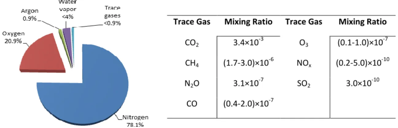
release from crustal material and degassing of the interior”.1 The next most abundant constituent is water vapour (H2O) whose concentration is highly variable and controlled by water evaporation and precipitation. In spite of their minor concentrations, the remaining constituent gases, also known as trace gases, which include some nitrogenated compounds like NOx and N2O, play a

5 fundamental role in the Earth’s radioactive balance and in the chemical properties of the atmosphere. The values of each atmosphere’s constituent are shown in Figure 1.1.

Trace Gas Mixing Ratio Trace Gas Mixing Ratio CO2 3.4×10-3 O3 (0.1-1.0)×10-7

CH4 (1.7-3.0)×10-6 NOx (0.2-5.0)×10-10

N2O 3.1×10-7 SO2 3.0×10-10

CO (0.4-2.0)×10-7

Figure 1.1- Composition (% v/v) of Earth's Atmosphere, adapted from Jacob et al.30

The trace gases concentrations have changed rapidly and remarkably over the last two centuries, mainly due to anthropogenic activity. Observations have shown that the composition of the atmosphere is changing on a global scale. In fact, recent measurements, combined with analyses of ancient air trapped in bubbles in ice cores, provided the record of a dramatic global increase on the concentrations of gases such as CO2, CH4, N2O and various halogen-containing compounds.1 These gases, also known as “greenhouse gases”, are able to absorb infrared radiation from the Earth’s surface and radiate a portion of it back to the surface, acting as atmospheric thermal insulators.

The overall effect of a gas on the Earth’s temperature is measured by the global warming potential (GWP). As can be seen in Table 1.1, N2O is one of the most important and powerful greenhouse gases, with a global warming potential 296 times higher that of CO2; this is a result of its long residence time and its relatively large energy absorption capacity per molecule. Moreover, as it will be discussed later, N2O can perturb in a large scale the atmospheric chemistry.

Table 1.1- Global Warming Potential (GWP) and lifetime of some pollutants, adapted from Seinfeld

et al.1

Chemical species Lifetime (year) 100-years GWP

CH4 8.4 23 N2O 120 296 CF4 >50000 5700 C2F6 10000 11900 SF2 3200 22200 HFC-23 260 12000 CO2 - a) 1 a)

6

As mentioned before, the trace gases contribute to the Earth’s radioactive balance but, also have an important effect in human and environmental health. According to the WHO, air pollution has caused approximately 800.000 deaths and 4.6 million lost life-years worldwide. Nonetheless, these numbers are expected to be worse than these estimations since they were estimated mainly based on the United States (US) data and extrapolated worldwide, and it is well known that this problem is not equally distributed globally, being one of the world highest levels of air pollution found in Asian megacities.31

As history shows, a serious consequence of exposure to air pollution occurred in the mid-20th century when cities of Europe and US suffered air pollution episodes, like the infamous 1952 London smog, that resulted in many deaths and hospital admissions32, 33 and the recurrent smog occurrences in Los Angeles. Although the biological mechanisms are not fully comprehended, many epidemiological studies suggest34-38 a close link between air pollution and various health outcomes (respiratory symptoms, mortality, cancer and congenital heart disease). Air Pollution may also lead to environmental degradation such as: Direct plant damage, caused by gases and acids in direct contact with leaves and needles; Soil acidification, mostly produced by acid rain but also by the harvesting of biomass by the forestry industry; Excess nitrogen, caused by nitrogen deposition leading to the fast growth of trees crowns, faster than their root systems, and Warmer climate, originating sea level rise and a probable increase in the frequency of some extreme weather events.39

These pollution levels seem to be linked to social and economic development mainly due to the increase use of fossil fuels for transport, power generation and products fabrications. Consequently, clean air legislation needed to be carried out in order to reduce the emission of pollutants and the infamous 1952 London smog was an important turning event in air quality control and legislation.33 In 1956, the Clean Air Act (CAA) authorized air pollution research and left the responsibility for air pollution control to state and local governments. It was only with the 1970 CAA amendments that this responsibility was spread to other entities like the Environmental Protection Agency (EPA) created in the US.40, 41 EPA established national ambient air quality standards to protect health and welfare and required that these standards should be achieved and maintained across the country. Other important events concerning air quality occurred during the following 30 years where the European Union (UE) and other international organisations exerted strong influence.33

7 Table 1.2- Estimate of Global Tropospheric NOx emission in the year 2000, adapted from Seinfeld et al.1 (1 Tg nitrogen=1012 g nitrogen).

Sources Emissions

(Tg nitrogen/year)

Fossil fuel combustion 33.0

Aircraft 0.7

Biomass burning 7.1

Soils 5.6

Lightning 5.0

Even though all the changes and improvements seen in the past 50 years, air pollution is still a major concern mainly due to some recurring episodes of summer smog in major cities, the well-known ozone hole over the Antarctic or even a controversial issue, climate change.

1.3- Nitrogenated Compounds

As stated before, nitrogenated compounds are considered one of the most important air pollutants. Nonetheless, N2, the most abundant compound (78%) on Earth’s atmosphere, is

practically inert and, due to its chemical stability, is not involved in the atmosphere’s chemistry; hence it is not an air pollutant. However, it becomes very useful to most organisms when it is fixed or converted to a form that can be used by the organisms. N2 fixation can either occur by natural, industrial or combustions methods. The most important result in the form of N2O, nitric oxide (NO), nitrogen dioxide (NO2), nitric acid (HNO3) and ammonia (NH3).1 Usually NO, NO2, N2O and other less common combination of nitrogen and oxygen (N2O4 and N2O5) are known as NOx

(oxides of nitrogen). The EPA defines NOx as “all oxides of nitrogen except N2O”.42 For

simplification, this nomenclature will be adopted in this work.

NOx are among the most important molecules in atmospheric chemistry as they play a

central role in the nitrogen cycle (see Figure 8.1 in the appendix A) and, due its high reactivity, they are the main reason for ground level ozone, acid rain and smog.1 The two primary NOx are NO and NO2.

NO is a colourless, poisonous gas that presents several adverse health effects, such as eyes and throat irritation, nausea, headache and gradual strength loss. In addition, prolonged exposure can cause violent coughing, difficulty in breathing and cyanosis.2 In extreme cases it could even be fatal. NO2 is a reddish brown and highly reactive gas and strong oxidant agent that has a suffocating odour. It is also highly toxic,

hazardous and able to cause delayed chemical pneumonitis and pulmonary edema.2 Combustions are by far the largest source of NOx, as shown in Table 1.2. Coal-fired electric

power plants and industrial combustion are the highest sources of NOx. Furthermore, motor

vehicles and other forms of transportation, including ships, airplanes and trains have also a

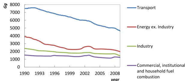
8 57% 5% 4% 4% 1% 29% Agriculture Transport Energy Industry Other Waste Chemical Industry large contribution.40, 43 Nevertheless, NOx emissions have decreased in the last 20 years in Europe,

as depicted in Figure 1.2, mainly due to the emergence of strict legislation and directives, like EURO 5 for transports and The Large Combustion Plant and the Integrated Pollution Prevention and Control for industry.44

Figure 1.2- Evolution of NOx emissions by source sector in the EU adapted from the 2011 Air Quality report44 (1 Gg=1000 tonnes/year).

N2O is a colourless gas, commonly referred as the “laughing gas” and it is widely employed as an anaesthetic. Also, N2O is inert in the troposphere but in the stratosphere, it turns into the major input of NO, becoming an important natural regulator of stratospheric O3 and,

therefore, N2O is the main responsible for the O3 depleting.45 Nonetheless, about 90% of N2O is destroyed in the stratosphere by photolysis (see Figure 8.1 in the appendix A). N2O is emitted predominantly by biological sources in soils and water,1 while agriculture and chemical industry are the main anthropogenic sources, as depicted in Figure 1.3.

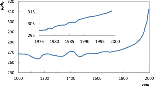
Nowadays, there is no official governmental legislation for the emission of this pollutant therefore, its increase is expected to take a rate of 0,26% per year due to anthropogenic emissions.46 As a matter of fact, ice core records of N2O showed a preindustrial mixing ratio of about 276 ppb, while in 2000 it was 315 ppb and in 2005 it was 319 ppb (Figure 1.4). In addition, it is expected to reach levels of 360-460 ppb by the year 2100, 11-45% higher than the actual concentration, mainly due to the larger contribution of chemical industry. One of the main

0 1000 2000 3000 4000 5000 6000 7000 8000 1990 1993 1996 1999 2002 2005 2008 Gg year Transport

Energy ex. Industry

Industry

Commercial, institutional and household fuel combustion

Figure 1.3- Total annual anthropogenic N2O emission in the

9 contribution comes from the HNO3 production where N2O is formed, resulting in emissions of 400kT per year.46

Figure 1.4- Evolution of the atmospheric N2O concentration, adapted from Pérez-Ramirez et al.46

1.4- Control Methods for Nitrogenated Compounds

The technologies used for reducing NOx are divided in: i) primary control technologies or

combustion control and ii) secondary control technology or flue gas treatment. Primary control technologies are used to minimize the amount of NOx initially produced in the combustion zone

and involves a pre-treatment process and/or a process and combustion modifications, i.e., NOx is

reduced by taking advantage of the thermodynamics and kinetics of the process by, for example, reducing flame peak temperature, reducing oxygen concentration in the primary flame zone or even, using thermodynamic and kinetic balances to promote the reconversion of NOx back to N2

and O2. In the other hand, secondary control technologies are used to reduce the NOx present in

the exhaust gas from the combustion zone, i.e., from the post-combustion stream. They focus mainly on converting NOx into N2 and O2 using a reducing agent with or without a catalyst, or

through the absorption of the species of interest.40

Both technologies are often used in a wide variety of combinations to achieve desired NOx

emission levels at optimal cost but, it is important to take into account that the performance of the individual technologies is not additive and varies for each combustion process.40

The most common techniques used for primary control are: Low-Excess Air Firing, Over Fire Air (OFA), Flue Gas Recirculation, Reducing Air Preheated, Reducing Firing Rate, Water/Steam Injection, Burners Out of Service (BOOS), Reburning, Low-NOx Burner (LNB), Ultra Low-NOx Burner, Injection Timing Retard, Air/fuel Ratio Changes, Low Emission Combustion, Low-NOx

250 260 270 280 290 300 310 320 1000 1200 1400 1600 1800 2000 ppb v year 295 305 315 1975 1980 1985 1990 1995 2000

10

Burners with Indirect Firing, Low-NOx Precalciners, Mid-kiln Firing. For secondary control there are: Selective Non-catalytic Reduction (SNCR), Selective Catalytic Reduction (SCR), Reburning, Low-Temperature Oxidation using Ozone, SconoxTM, Low-Temperature Oxidation with Absorption (LTOA) and Biosolids Injection (BSI).40, 43 In Table 1.3 is listed a summary of some NOx control techniques and respective removal efficiency.

Table 1.3- Summary of NOx removal efficiency reported in the literature for diverse techniques.

Techniques Reported NOx removal efficiency

Low-Excess Air Firing 15-55%a)

Low NOx Burner 40-65%

a) 14-50%b)

Over Fire Air Additional 10 to 25% beyond LNBb)

Selective Non Catalytic Reduction 30-50%

a) 10-90%b)

Selective Catalytic Reduction 70-90%

a) 80-95%b)

Reburning 58-77%

a) 39-67%b) Low Temperature Oxidation with Absorption 99%a)

Burners Out Of Service 15-30%a)

Water/Steam Injection 20-30%a)

Biosolids Injection 50%b)

Injection Timing Retard 15-30%b)

Air/fuel ratio Changes 50+%b)

Low Emission Combustion 80+%b)

a)

Data from Schnelle. et al.40; b) Data from Srivastava et al.43

As shown in Table 1.3, some techniques achieve high NOx reduction but require proper care

to be taken in operating and maintaining the combustion process in order to attain the desired range of emissions. SNCR and SCR, besides LTOA, provide high NOx reduction so they are the most

popular control techniques along with LNB and OFA.43

On the other hand, HNO3 production is one of the main contributors for increasing N2O emissions, as it is formed during its synthesis, being then released from reactor vents into the atmosphere. Production of weak HNO3 is based on the Ostwald process and consists on some basic chemical operations: Catalytic oxidation of NH3 with air into NO; Oxidation of NO into NO2 and Absorption of NO2 in water to produce HNO3. The N2O formation depends totally on the NH3 oxidation process and it can result in other products depending on the process temperature, as follows:

11 → {

_{Eq. 1.1}

For the three previous paths, at low temperatures (423-473 K) N2 is the principal product formed, while at higher temperatures N2O formation is initiated, reaching its maximum at 675 K. The desired product, NO, starts at 573 K and its yields continuously increase with temperature. Catalyst selectivity is important as well as composition and state (age), for achieving NO yields of 95-97%, typical values under industrial conditions. There is still others undesired reactions, involving by-products and unreacted NH3, that can lead to an increase of N2O emissions.46 Thus, a great effort has been made to develop N2O abatement systems capable of achieving high efficiency (>90% N2O conversion) and selectivity (0.2% NO loss).

Nowadays, apart from process optimization, that will not be addressed here, only a few techniques, such as Thermal Decomposition, SCR, SNCR and Catalytic Direct Decomposition, are used for N2O abatement from industrial sources.46 Thermal Decomposition of N2O is based on raising the temperature of the exhaust gases to the required 1023-1273 K, at this point it decomposes in N2 and O2.47 However, this technique seems to be prohibitive because it requires a high-temperature heat exchanger which can represent a huge investment and operational costs. Thus, other techniques like SNCR and SCR are preferred. They were already referred as control techniques for NOx and both are based in the use of a reducing agent in the presence or not of a catalyst (normally metal-zeolites). Propane, propene, natural gas or NH3are normally used as reducing agents for SCR, while hydrogen (H2), natural gas or naphtha are used for SNCR. SNCR has conversion efficiencies of about 70% while SCR has highest (up to 100%), but requires an optimal temperature control (650-793 K) and a periodically replacement of the catalyst due to its high sensitivity to impurities present in the treated effluent.46 Finally, Catalytic Direct Decomposition is based in the N2O decomposition without a reducing agent, so they could be more attractive and economical than the previous options. However, none of the studied catalyst showed a good activity and stability under realistic industrial conditions. Some of the catalysts already studied include transition (Cu, Co and Ni) and noble metal-based catalysts (Rh, Ru and Pd) on different supports (ZnO, CeO2, Al2O3, TiO2, ZrO2, calcined hydrotalcites and perovkites).46

12

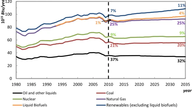
1.5- Control Methods Insufficiency

The available techniques, already implemented in industry and capable of reducing nitrogenated compounds to values permitted by the actual legislation, do not guarantee the total pollutants removal and all present several problems and limitations. In addition, it is expected that the dependency on fossil fuels will be maintained as recently showed by the 2012 Annual Energy Outlook report48 (Figure 1.5). These projections are only for the US, however this scenario would not be very different from the rest of the world.

Figure 1.5- US primary energy consumption forecast till the year 2035 adapted from the Annual Energy Outlook 2012.48

Moreover, stricter legislation will continue to appear and environmental problems will not disappear leading to an increasing need for better and more efficient control methods. A possible solution could be the development of a new control method that could be combined with the existent techniques, for example an absorption or membrane process. These techniques could replace or be combined with existent control strategies in industrial sources such as large boilers, furnaces and fired heaters, combustion turbines, large internal combustion engines, cement kilns and exhaust streams from HNO3 production. The potential uses of these two techniques would imply the use of a resistant material and a high boiling temperature solvent like ILs.

0 20 40 60 80 100 120 1980 1985 1990 1995 2000 2005 2010 2015 2020 2025 2030 2035 10 15 B tu /yea r year

Oil and other liquids Coal

Nuclear Natural Gas

Liquid Biofuels Renewables (excluding liquid biofuels)

37% _32% 21% 20% 9% 9% 25% 25% 11% 7% 1% 4%

13

1.6- Ionic Liquids

ILs are salts composed of large organic cations and organic or inorganic anions that cannot form an ordered crystal and thus remain liquid at or near room temperature (by definition are liquid at temperature below 373 K). Although the combination of cations and anions allows one the synthesis of more than 106 different ILs, only a small amount (≈1000) of these compounds are described and characterized in literature.49 In fact, most of the ILs studied are based on the ammonium, phosphonium, pyridium or imidazolium cation, and on the tetrafluoroborate [BF4]-, hexafluorophosphate [PF6]-, trifluoromethylsulfonate [CF3SO3]- or bis(trifluoromethylsulfonyl)imide [NTf2]- anion.49 Illustrative examples of some of these cations and anions are showed in Figure 1.6.

Figure 1.6- Cations and anions commonly used to form ILs.

These unique compounds were first reported by Paul Walden50 in 1914 when he studied the physical properties of ethylammonium nitrate ([EtNH3][NO3]). His intention was to investigate the electric conductivity and the molecular size of some organic ammonium salts.49 Even though his clear exposition and discovery of a new class of liquids, only in 1934 were they cited in a patent where it was claimed that they could be used for dissolving cellulose.51 Over the years that followed, more studies were carried out and, by the mid-1990s, the concept of ILs was well-known mostly for their electrochemical applications.49

The attention of a larger community was attracted when the first water and air stable ILs were developed and these new solvents were touted as “green” and they emerged as “designer solvents”. This designation was first used by Seddon et al.52 when reporting the use of ILs as solvents for reaction optimization, achieving control over yield and selectivity. Since a large number of cationic and anionic structures combinations are possible, desired physicochemical properties of ILs for a particular process can be easily tuned and/or obtained by manipulating the ions that compose them.52 For instance, hydrophobicity, viscosity or density can be adjusted by changing the alkyl chain of the cation,53-56 or their water miscibility by changing the anion,49 or a pyridinium imidazolium tetrafluoroborate bis(trifluoromethylsulfonyl)imide

14

more important property for this work, the gas solubility can be manipulated by the anion/cation selection.5, 57

The ionic nature of these liquids results in several physical and chemical advantages over conventional and molecular organic solvent such as negligible flammability and vapour pressure, thermal stability and highly solvating capacity either for polar and nonpolar compounds.58-60 _These unique characteristics raised the attention both from the academia as well as from the industry.

Due to the ILs unique features, they have been intensively applied in different areas like multiphase bioprocess operations,61 chromatographic separations,62 mass spectrometry analysis,63 batteries and fuel cells,64 solar cells,65 separation of biomolecules,66 organic synthesis,67 chemical reactions,68 catalysis,69 liquid-liquid extractions of metal ions70, 71 and organic compounds.72, 73 Furthermore, their unique and outstanding characteristics could allow them to be used in several control process for pollutant, as absorption solvent in an extraction process or as stationary phase in a membrane process, just to mention some. In fact, a large number of studies have been performed concerning pollutants solubility on ILs, namely for CO2,17-19, 74-83

CH4,6, 84-88 H2S,83, 89 SO2,8, 90CO,76, 91-93 and NH3.8 These studies have shown good results at low

temperatures, indicating that this class of solvents are feasible to be used to capture and/or separate these pollutants. However, no studies have been made for NOx and, up to now, only four

studies with N2O were reported.5, 14, 16, 18 Of these studies, the most interesting is the study conducted by Revelli et al.14 where the solubility of N2O in five imidazolium-based ILs was investigated, showing that it was possible to dissolve, at low pressure, up to 105 grams of N2O per kilogram of IL.

The ILs exclusive characteristics and good solubility towards various gases make them promising agents for the capture of nitrogenated gases. However, a more complete solubility study is needed in order to develop techniques for reducing these compounds. Moreover, solubility data are important to develop thermodynamic models and correlations able to describe and/or predict such systems and therefore to reduce the need for an exhaustive study. To this purpose, several different theoretical approaches, correlations and equations of state (EoS) have been already applied to ILs + gases systems. Those with the best results are the soft-SAFT EoS,22-25, 94, 95_

15

1.7- Soft-SAFT EoS

Among the EoS used to describe gas solubilities in ILs, the Statistical Associating Fluid Theory (SAFT)97-100 is becoming very popular due it success in predicting not only gas solubilities but also other ILs thermodynamic properties.95 _{This theory has generated a family of SAFT-type} equations based on Wertheim’s first-order thermodynamic perturbation theory (TPT1) for associating fluids.101-104 The soft-SAFT EoS, proposed by Vega and co-workers,21, 26, 105, 106 is one of the most successful equations of this type. They were able to successfully predict the phase equilibrium behaviour of binary and ternary mixtures involving noassociating compounds like n-alkanes and 1-n-alkanes, and associating compounds like 1-alkanols,21 as well as their critical lines and partial miscibility.106 Later, the same study was extended with success for some heavy n-alkanes by Pàmies et al.26 Recent works,22-25 extended the soft-SAFT EoS applicability to more complex fluids, like ILs, with great success. Contrarily to classical models, which in most cases are based on the use of several temperature and composition dependent parameters, SAFT-type equations are able to describe IL + gas systems with a simple model and non-temperature dependent parameters.94 Moreover, classical models required the use of ILs’ critical properties that, lacking a better expression, are challenging to determine, making its determination possible through indirect estimated models that present large uncertainties.94

As all SAFT-type equations, the soft-SAFT EoS is written in term of the residual Helmholtz energy ( , defined as the molar Helmholtz energy of the fluid relative to that of an ideal gas at the same temperature and density. This energy can be calculated by the sum of each independent microscopic contribution. The general expression of the SAFT equation is:

Eq. 1.2

where the superscripts ref, chain, assoc and polar refer to the contribution from the reference term, the formation of the chain, the association and the polar interactions, respectively. A hypothetical model of an associating molecule modeled by the SAFT approach is depicted in Figure 1.7, where the number of segments (m), the segment size (σ), the dispersive energy between segments (ε/kB), the energy (εHB/kB) and volume (kHB) of association per site are

16

Figure 1.7- Molecule model within the soft-SAFT approach.

While the original SAFT uses a reference fluid based on hard-spheres, the soft-SAFT EoS uses a Lennard-Jones (LJ) spherical fluid, a “soft” reference fluid, which takes into account the repulsive and attractive interactions of the segments forming the chain and is modelled by the Lennard Jones EoS.107 This equation was obtained by fitting simulation data in Benedict-Webb-Rubbin EoS and posterior parameters determination and can be extended to mixtures by applying the van der Waals one-fluid theory (vdW-1f).108 The expressions for the size and energy parameters are:

∑ ∑

∑ ∑ Eq. 1.3

∑ ∑

∑ ∑ Eq. 1.4

where the subscripts and refers to the species in the mixture, and the unlike parameters, and , are calculated using the generalized Lorentz-Berthelot combining rule. The corresponding expressions are:

_{Eq. 1.5}

√ _{Eq. 1.6} where and are the binary adjustable parameters for the species and . These parameters are used to correct possible deviations in molecular size and energy of the segments forming the two compounds in the mixture. Moreover, when both binary adjustable parameters are set to 1, soft-SAFT EoS is used in a pure predictive manner.

The reference term usually varies in different SAFT’s versions. On the other hand, the chain and association terms are normally identical and are derived from the Wertheim’s theory (TPT1):

_{∑ (}

_{Eq. 1.7}

_{∑ (∑ )}

17 where is the molecular density, is the Boltzmann’s constant, is the temperature, is the molar fraction of component , m is the chain length, is the radial distribution function of a fluid of LJ spheres at density and evaluated at the bond length , is the number of association sites in component , and is the mole fraction of molecules of component nonbonded at site , which extends over all compound in the mixture.

Finally, main polar interactions can also be taken into account in the model by introducing a new parameter, the quadrupole moment, Q. The calculation of this parameter is based on setting the fraction of segments in the chain that contains the quadrupole, and it is defined in the model as . Usually, these two parameters are previously calculated and fixed, and are correlated by the following equation:

_{Eq. 1.9}

where is the experimental quadrupole for the molecule of interest and and are molecular parameters for the model. Moreover, its use is required when modelling some fluids of linear symmetrical molecules like carbon dioxide, nitrogen and acetylene, and others like benzene, ethylbenzene, n-propybenzene and toluene, where this property is important.12, 22, 23, 27, 109

Although the quadrupole moment for N2O was already studied,110, 111 it remains unknown its effect on the soft-SAFT EoS prediction.

In order to apply Sof-SAFT EoS for a particular system, a molecular model for each compound must be chosen (sites for each molecule and allowed interactions among the sites) as well as obtain the molecular parameters. In this sense, molecular parameters of pure compound are calculated by fitting experimental data for vapour pressure and saturated liquid density over a determinate range of temperature using the functions21:

( ⁄ _{∑ [ ( )] Eq. 1.10} ( ⁄ _{∑ [ ( )} ( )] Eq. 1.11 where is the number of experimental points, , , are the vapour pressure, the liquid density and the temperature corresponding to the experimental point , and , , _{are the chemical potentials of the liquid and vapour phase and the saturated liquid density,} respectively, predicted by the EoS at the temperature and pressure . These two functions are minimized using the Marquart-Levenberg algorithm112 and the process stopped when or are less than . For binary mixtures, the same fitting procedure is used along with the two binary parameters given in Eq. 1.5 and Eq. 1.6, and the next two functions:

( _{∑ [ ( )]}

18

( _{∑ [ ( )]}

_{Eq. 1.13}

Generally, ILs are well modelled by using all five molecular parameters (m, σ, ε/kB, kHBand

19

21

2.1- Introduction

The selection of a reliable coarse-grained model able to represent the basic physical features of the compound to be described stands as a key element for the accurate predictions from any molecular-based EoS. soft-SAFT EoS relies on the pre-adjustments of molecular parameters for each pure compound. The molecules are represented through the molecular parameters: m, the chain length; σ, the segment size; ε, the energy parameter of the segments making the chain; Q, the quadrupolar moment; xp, the fraction of segments in the chain that

contains the quadrupole; kHB, the volume of association and εHB/kB, the association energy per

site. Additionally, the description of the pure compound vapour pressure and liquid density is evaluated by the percentage average absolute deviation (%AAD), defined as the difference between experimental data and the predictions given by soft-SAFT EoS, and was calculated by:

| ∑ | Eq. 2.1

where N stands for the number of points considered and the subscript exp and calc, are the experimental and calculated values by the model, respectively, for the studied property, Z.

2.2- ILs Molecular Parameters

Although successfully applied for a wide set of compound families, like associating and non-associating hydrocarbons,21, 106, 113 polymers27, 109 and perfluoalkanes,12 soft-SAFT EoS has only recently been extended to ILs by Vega and co-workers. 22-25

Imidazolium-based ILs with PF6 and BF4 anions were modelled22, 25 as LJ chain with one associating site, “A”, where the “A” site represents the specifics interactions due to the IL chargers and asymmetry (Figure 2.1). On the other hand, imidazolium-based ILs with NTf2 anion were modelled23-25 with three associating sites, one “A” and two “B” sites, where the “A” would mimic the specific interactions due the nitrogen atom with the cation and the “B” sites would represent the delocalized charge due the oxygen atoms on the anion (Figure 2.2). Also, only AA or AB interactions, between different ILs molecules are allowed.

22

Figure 2.1- Proposed association scheme for [C4mim][BF4] by Andreu et al.22

Figure 2.2- Proposed association scheme for [C4mim][NTf2] by Andreu et al.23

Once the ILs association scheme was selected, the molecular parameters, m, σ, ε/kB, kHBand

εHB/kB were determined. Following the Vega and co-workers suggestion, the association

parameters (εHB/kB =3450 and kHB=2250) were transferred from those of 1-alkanols,114 reducing

thus, to a minimum, the number of fitted molecular parameters. Afterwards, the remaining molecular parameters (m, σ and ε/kB) were obtained by fitting them to experimental density data

at atmospheric pressure.115, 116 Furthermore, recently, Llovel et al.24 recalculated the molecular parameters for the NTf2 family using the previously discussed scheme of association and new available experimental density data.117 In addition to that, similarly to what was done for other compounds,21, 27, 109 a correlation between the molecular parameters and the molecular weight of the ILs was established for the PF6, BF4 and NTf2 families,22, 2324 improving the predictive ability of the soft-SAFT EoS.

The adjusted molecular parameters for [C4mim][BF4] and [C4mim][NTf2] are listed in Table 2.1 and allowed a good description of the ILs density, as depicted in Figure 2.3, with an %AAD of 0.31% and 0.06%, respectively.

Table 2.1- Molecular parameters for [C4mim][BF4]and [C4mim][NTf2] taken from the literature.22, 24

m σ (Å) ε/kB (K) ε HB/kB (K) k HB (Å3) [C4mim][BF4] 4.495 4.029 420.00 3450 2250 [C4mim][NTf2] 6.175 4.211 399.40 3450 2250

A

A

B

B

23 Figure 2.3- [C4mim][BF4] (a) and [C4mim][NTf2] (b) temperature-density diagrams.117, 118 Solid lines represent soft-SAFT EoS predictions.

The set of molecular parameters used allowed a good description of the phase behaviour of some compound such as CO2 in [C4mim][BF4]22 and CO2, Xe, H2, H2O, methanol and ethanol in [C4mim][NTf2].23, 24 Therefore, these set of parameters will be used for modelling binary mixtures in this work.

Molecular parameters for [C4mim][SCN], [C2mim][CH3OHPO2] and [C4mim][N(CN)2] were not available in the literature. Therefore, they are here determined for the first time.

Following the above mentioned approach, the ILs were modelled as a LJ chain with two association sites; one “A” and one “B” site, as depicted in Figure 2.4.

Figure 2.4- Scheme of association adopted in this work for the ILs [C4mim][SCN] (a), [C2mim][CH3OHPO2] (b) and [C4mim][N(CN)2] (c).

(a) _(b) (a) (b) (c)

A

A

B

A

B

B