RBRH, Porto Alegre, v. 23, e55, 2018 Scientific/Technical Article
https://doi.org/10.1590/2318-0331.231820170165
A coupled system based on Differential Evolution for the determination of Rainfall
intensity equations
Um sistema acoplado baseado em Evolução Diferencial para determinação de equações de chuvas intensas
Guilherme José Cunha Gomes1 and Eurípedes do Amaral Vargas Júnior2
1Departamento de Estradas de Rodagem do Espírito Santo, Vitória, ES, Brasil
2Pontifícia Universidade Católica do Rio de Janeiro, Rio de Janeiro, RJ, Brasil
E-mails: guilhermejcg@yahoo.com.br (GJCG), vargas@puc-rio.br (EAVJ)
Received: October 10, 2017 - Revised: August 05, 2018 - Accepted: September 24, 2018
ABSTRACT
Rainfall intensity equations are fundamental in hydrological studies of road design, which require a project rainfall definition to estimate the project flow and the subsequent design of the hydraulic structure. This paper develops an integrated framework for
rainfall intensity equations analyses from global optimization via Differential Evolution. The code was specially developed to facilitate
the Gumbel model adjustment in the frequency analysis of annual series, as well as the intensity-duration-frequency model fit, without
prior knowledge about the parameters of both models. The developed system was evaluated by using Markov chain Monte Carlo
simulation, that search efficiently the model parameter space in pursuit of posterior samples and the posterior prediction uncertainty for both models. The results indicate that simulations are shown to be in good agreement with the measured flow and precipitation
data. The optimal parameters obtained with the developed framework agreed with the maximum a-posteriori value of the Monte Carlo
simulations. The paper illustrates explicitly the benefits of the method using real-world precipitation data collected for a hydrologic
study of a highway design.
Keywords: Precipitation; Rainfall intensity equations; Global optimization; Differential Evolution; Highway design.
RESUMO
As equações de chuvas intensas são fundamentais em estudos hidrológicos de projetos rodoviários, os quais requerem a definição
da chuva de projeto para estimativa da vazão de projeto e o posterior dimensionamento da estrutura hidráulica. Neste trabalho, desenvolveu-se um sistema computacional para a obtenção da equação de chuvas intensas, a partir de otimização global via Evolução Diferencial. O sistema foi especialmente projetado para facilitar o ajuste do modelo de Gumbel na análise de frequência de séries anuais, bem como o ajuste do modelo da curva intensidade-duração-frequência, sem que o usuário necessite conhecimento prévio sobre os parâmetros de ambos os modelos. Simulações Monte Carlo via cadeia de Markov foram realizadas para avaliar a metodologia desenvolvida através da distribuição posterior dos parâmetros e da incerteza preditiva de ambos os modelos. Os resultados obtidos indicaram bons ajustes para os modelos de Gumbel e da equação de chuvas intensas com o uso da otimização global via Evolução Diferencial, uma vez que os parâmetros ótimos obtidos pelo sistema concordaram com o valor máximo a-posteriori oriundo das simulações Monte Carlo. Um estudo de caso envolvendo a obtenção da equação de chuvas em um estudo hidrológico de projeto rodoviário ilustram a usabilidade e aplicabilidade do sistema e da metodologia desenvolvida.
INTRODUCTION
Rainfall controls a very wide range of processes on the Earth´s surface. However, the behavior of exceptional rainfall is hard to determine, and is generally handled in a probabilistic way. These rains can be determined through rainfall intensity equations, which are broadly utilized for dimensioning drainage structures with different purposes, including agricultural (VIVEKANANDAN, 2017) and urban drainage systems (SABÓIA et al., 2017), channels (WRIGHT; SMITH; BAECK, 2014), and engineering structures in road projects (KANG et al., 2009). A precise characterization of rainfall intensity equations is therefore vital for the appropriate sizing of different drainage structures.
Different probabilistic models (e.g. normal, log-normal, and Gumbel) can be used to obtain an event (rainfall or discharge)
that can be exceeded, on average, once at every specified period of
time (usually years). Such models, non-linear in their parameters, consist in the probability cumulative functions of each statistical distribution. From the historical observations of the event (e.g. annual maximum daily precipitations), the statistical model is mixed with the observed events through the estimation of parameters that provide better adjustment of the employed model to the observed rainfall data. Among the statistical distributions, the Gumbel model is widely used for estimating precipitation or discharge data regarding a certain return period (Tr). A detailed description of the adjustment of statistical distributions to data on rainfall events is provided by Tucci (1993), including different techniques for estimating the parameters of the models. After this optimization process is completed, the maximum daily precipitations are determined for different values of Tr.
The rainfall intensity equation, also called intensity-duration-frequency (IDF) curve, provides estimates of rainfall intensity concerning different rainfall durations and different values of Tr. The IDF relations, obtained from the disaggregation of the annual maximum daily precipitations, constitute one of the elements necessary for calculating the design discharge, i.e. the discharge employed for the sizing of drainage structures. Different models for the IDF curves have been proposed in the literature (KOUTSOYIANNIS; KOZONIS; MANETAS, 1998) and, like the probability cumulative functions of the statistical distributions, they require techniques for estimating the parameters of adjustment between calibration data and models.
Different techniques are available for estimating the parameters of the Gumbel model. These techniques include the method of moments (TUCCI, 1993; MADSEN et al., 2002; MOHYMONT; DEMARÉE; FAKA, 2004), maximum likelihood estimation (CHOW; MAIDMENT; MAYS, 1988; FADHEL et al., 2017), approximate Bayesian computations (DEMIRHAN, 2017), among others. For the IDF equations, the search for the model parameters can be performed through linear regression with the linearization of the model (SILVA et al., 2012), besides iterative methods or non-linear regressions, such as the Gauss-Newton (GARCIA et al., 2011) and Levenberg-Marquardt models (PENNER; LIMA, 2016). These last techniques are also called methods of local optimization, in which, in order to start the optimization process, there must be an initial estimate of the parameters that needs to be relatively close to the optimal values.
Regarding models that are non-linear in their parameters, such as the Gumbel model and the IDF curve, it is widely established in the literature (VRUGT, 2016) that methods of global optimization
are more efficient for the calibration of models. Among the available
techniques, the Differential Evolution has the advantage of easily handling non-differentiable, highly non-linear, and multi-modal functions (STORN; PRICE, 1997).
While in the literature a lot of effort has been made in calibrating the Gumbel and IDF models through techniques of local optimization, little attention has been given to the inference of parameters through techniques of global optimization. Application examples of global optimization techniques in the obtainment of the IDF relations involve the utilization of genetic algorithms (KARAHAN; AYVAZ; GURARSLAN, 2008) and particle swarm (KARAHAN, 2012). In this article, we present an alternative computer system for the global optimization of the Gumbel model and the rainfall intensity equation. By using the method of global optimization via Differential Evolution, the program provides the parameters for both models with no need of estimating an initial value for them, using as input only the annual maximum precipitations. Markov chain Monte Carlo simulations using the DREAM software (VRUGT, 2016) illustrate the benefits of using the system. Furthermore, the same platform provides a set of computational tools, including the direct obtainment of the design discharge and the visualization of the output data.
The remainder of the article is organized as follows: The next section presents the different elements of the system developed in MATLAB. Then, it is shown a case study regarding the obtainment of the rainfall intensity equation of a project for dimensioning a drainage structure (bridge) in a road located in state of Espírito Santo, Brazil. At last, this article draws to a conclusion
with the summary and discussions of the main findings.
SYSTEM DESCRIPTION
In this section, the paper presents an automatic system for determining rainfall intensity equations using the optimization of the Gumbel model (Toolbox Gumbel) and of the IDF curve (Toolbox IDF). The system was developed in MATLAB, coupling two global optimization algorithms via Differential Evolution in such a way that the users do not need to assign values to the parameters. In addition, the framework has built-in capabilities for pre and post-processing for program initialization and visualization of the results. After obtaining the rainfall intensity, another module was included (HU Toolbox) with the implementation of the synthetic unit hydrograph method for the obtainment of the design discharge. Figure 1 shows a schematic chart of the developed system, indicating the program’s different tools, as well as a summary of the input and output data.
The Toolbox Gumbel is started from an Excel spreadsheet (.csv) containing the years in which the data were obtained and the annual maximum precipitations (in millimeters). Thereafter, the code initiates the frequency analysis, the adjustment of the precipitation values to the Gumbel probability distribution, and the disaggregation of maximum daily rainfall into hourly rains. Besides the precipitations, it is possible to use the same procedure
The Toolbox IDF performs the adjustment of the IDF curves and the generation of the rainfall intensity equation. All of the previous steps are performed so that the users do not have to input any values, except for the spreadsheet that contains the annual maximum precipitations.
The Toolbox HU is an option the user has for determining the design hydrograph using the triangular synthetic hydrograph method. In this research, only the Toolbox Gumbel and the Toolbox
IDF tools are going to be detailed, since they specifically handle
optimization and automation routines of hydrological studies. Details about the Toolbox HU shall be discussed in another publication. Note that, to obtain the design discharge, it is necessary
to provide the system with five additional pieces of data, i.e.: the
area of the basin (A), the channel length (L) and declivity (H), the curve number parameter (CN) of the Soil Conservation Service (SCS) method from the United States Department of Agriculture (USDA), as well as the desired return period (Tr). The following
sections are going to detail the program summarized in the flow
chart shown in Figure 1.
Toolbox Gumbel
The program starts with the frequency analysis of the precipitations. The precipitations can be obtained from the National Water Agency (Agência Nacional de Águas - ANA)’s
website, where it is possible to find time series of rainfall and fluviometric stations located throughout the national territory.
The maximum precipitations are then organized in an Excel
spreadsheet (.csv file), as shown in Figure 1 (input data). The first
column of the spreadsheet gets the years of observation, and the
second one receives the annual maximum precipitations, associated with a certain duration, registered for the time series.
To exemplify the frequency analysis process, and, subsequently, the optimization process of the Gumbel statistical model, consider Table 1, which contains annual maximum discharges (Q) data from the river Mãe Luzia, located in Forquilhinha, published by Tucci (1993). The time series comprises 35 records of maximum discharges between the years of 1943 and 1985.
The annual maximum precipitations (Pmax) are then organized in descending order (P~max), and each value of P~max is assigned with its order number, m. Once the precipitations are ordinated, it is necessary to estimate their frequency or plotting position. Among Figure 1. General overview of the different elements of the system developed in MATLAB. The central column details the different stages of the program, whereas the left and right columns summarize the input and output data of the optimization processes, respectively. The consecutive stages of proposed modeling allow the user to obtain the rainfall intensity equation without dealing with parametrization.
Table 1. Annual maximum discharges in the river Mãe Luzia (Tucci, 1993).
Year Q Year Q Year Q
(m3/s) (m3/s) (m3/s)
1943 92.5 1955 261.0 1967 376.0
1944 228.6 1956 248.0 1976 252.0
1945 72.5 1957 256.5 1977 280.0
1946 180.0 1958 380.0 1978 470.0
1947 180.0 1959 221.4 1979 773.0
1948 350.0 1960 370.0 1980 880.0
1949 116.8 1961 360.0 1981 545.0
1950 216.0 1962 340.0 1982 117.0
1951 330.0 1963 480.0 1983 265.0
1952 241.2 1964 290.0 1984 121.0
1953 300.0 1965 216.0 1985 315.0
the most commonly used formulations in hydrology, Weibull’s plotting position considers the frequency in which an event e0 is equaled or exceeded by a random event e, and it is provided by:
( )0 /( ),
F e =m n 1+ (1)
where n is the number of observations of the time series and F e( )0 represents the exceedance probability (P{e≥e0}). The return period for each observation can be obtained via the relation (Tucci, 1993):
{ }
/
r 0
T =1 P e e≥ . (2)
The values of P~max and Tr, which may be plotted in a semi-log plot (square symbols in Figure 2a), are then used as input data for the global optimization of the Gumbel statistical model via Differential Evolution.
The Gumbel distribution has a vast application in hydrology in matters of adjustment of maximum precipitations and discharges. Although this distribution is frequently used in
the estimation of maximum precipitations, the Gumbel model may be inappropriate for calculating maximum daily rainfall (PAPALEXIOU; KOUTSOYIANNIS, 2012; PAPALEXIOU et al., 2013). For some maximum precipitation data, the Gumbel model may not adequately portray the events of larger magnitude. In this
case, verification tests, preferably those with adequate testing
power for discriminating the null and alternative hypotheses on the upper tail of the distribution (e.g. Anderson-Darling test), are required for evaluating the potential of the Gumbel distribution in the modeling of the maximum precipitations. If the Gumbel model is not appropriate, other models could be utilized, such as the log-normal distribution. Discussions about the adequacy of the Gumbel model to the rainfall events of larger magnitude are presented later on in the Discussions section. In this study, the Gumbel distribution was employed as a statistical model of the annual maximum daily precipitations merely as an application example of the developed system.
Global optimization
By using Gumbel’s probability cumulative distribution function, the annual maximum precipitations are determined according to the relation:
ln ln ,
max
r
1
P 1
T α β = − − − +
(3)
where α and β are scale and position parameters of the distribution, estimated via different techniques.
In this article, parameter estimation of α and β was performed using the Differential Evolution technique developed by Storn and Price (1997). Differential Evolution is a global optimization technique that quickly converges to the global optimum, besides being relatively easy to use and having few control variables. The method starts with the creation of a population X of N
parents, X={x x1, 2,…,xN}, through the sampling of the parameters’ prior bounds, xi∈d, where d denotes the dimensionality of the
search space. Each vector xi stores parameter values that simulate the model’s response. To exemplify, in the case of the optimization of the model presented in Equation 3, d 2= . The objective function
f(xi) is then calculated for each parent, i={1,...,N}, and stored in a vector F =
{
f x( ) ( )1 , f x2 ,..., f x( )N}
. The optimal solution ofthe optimization problem seeks to minimize or to maximize F. In order to create new generations from the population X, the following relation is used:
(
)
,i i DE j k
z = +x F x −x (4)
where zi is a dimension vector d containing a new generation stemming from the parent i; j and k are selected with no replacement of the set of integers {1 2, ,...,i 1 i 1− , + ,...,N}; and FDE∈(0 2, ] is a
factor that controls the diversity of the new generation. Once the new generation has been created, Z={z z1, 2,…,zN}, the values of the objective function can be calculated and stored in a vector
( ) ( ) ( )
{
}
1 , 2 ,..., N
G= f z f z f z .
The objective function employed was the root-mean-square error (RMSE), which measures the mean distance between the observed (Pmax) and simulated (Psim) precipitation values. This statistic Figure 2. (a) Adjustment of the Gumbel distribution to the
annual maximum discharges (Qmax) published by Tucci (1993);
(b) Comparison between the proposed DE method and the DREAM software. The dark and light-gray areas represent the
confidence intervals due to the uncertainty of the parameters,
has the same unit as the observations. The lower the RMSE value, the closer are the predictions of the n observed data. This metric can be calculated as follows:
( ) / ,
n
2
max sim
i 1
RMSE P P n
=
= ∑ − (5)
Finally, each parent is compared to its respective offspring. If Gi<Fi, then xi=zi and Fi=Gi, otherwise, the i-th descendant is rejected. If the maximum number of generations is not reached, it is necessary to return to Equation 4, otherwise the algorithm ends and uses the lowest-value parent in the objective function as the result of the optimization problem. A detailed description of the Differential Evolution algorithm can be obtained in Storn and Price (1997).
The version of Differential Evolution employed in the
system implemented in MATLAB includes crossover and verification
of the contours. In the crossover, after the implementation of Equation 4, for each new generation created, one vector of random numbers between 0 and 1 is generated (in the same dimension as vector zi). If the random number generated for that dimension is higher than the crossover rate, it is necessary to return to the value of the initial population, i.e. zi=xi. The crossover rate can be useful when the dimensionality of the search space is high. If the user wishes to disable the crossover function, all they have to do is maintain its value zero.
Offsprings generated with Equation 4 can fall outside the search domain, d. In order to ensure the permanence of candidates always in the search space region, the system includes
the verification of contours proposed by Vrugt (2016). In this
proposal, when a parameter or dimension of Z fall outside the search space d, the verification of the contours automatically reflects that dimension back inside the sample space, as detailed
by Vrugt (2016).
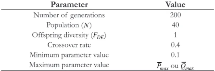
To verify the approach herein described for the optimization of the parameters α and β of the Gumbel model, the data presented by Tucci (1993), shown in Table 1 were used. The values employed for starting the optimization process are summarized in Table 2. 200 generations were employed with a population
N of 40 individuals, FDE=1 and a crossover rate of 0.4. For the sample space of the α and β parameters, a minimum value of 0.1 and a maximum value of Pmax (mean of the precipitation values recorded in the time series or mean discharge, Qmax) were
employed. This sample space, employed for both values of
α and β, comprises a broad search range, whereas this search
space is sufficient for obtaining the adjustment of the model to
the observed data. Again, one of the advantages of the present paper proposition is the agility in obtaining α and β, which are
automatically identified during the search.
Figure 2a shows the results of the Gumbel model optimization process with the system developed in MATLAB (solid line) through Differential Evolution (DE). The simulations were performed using the entire set of data, with no elimination of diverging data or outliers. The data presented by Tucci (1993), with the adjustment of parameters via method of moments, are also indicated in Figure 2, concerning different return periods (dotted line).
In order to evaluate the developed system, the DREAM software (VRUGT, 2016) was used to compare the estimates of the parameters for both the Gumbel model and the IDF curves. This multi-chain Markov chain Monte Carlo simulation algorithm automatically synchronizes the scale and the orientation of the proposed distribution. This is one of the reasons for which the
DREAM algorithm shows great efficiency in the sampling of
complex target distributions, as well as high-dimensional and multi-modal ones. Since DREAM has been considered state of the art in model calibration (VRUGT; BEVEN, 2018), this commercial program was used to test whether the convergence for the posterior distribution of the parameters was reached by the system developed in this study.
Figure 2b compares the modeled discharges using the DE method (solid line) and the DREAM algorithm (white triangles). It is possible to note that both techniques converge towards the
same result. The DREAM algorithm also enables the identification
of the intervals of 95% of predictive uncertainty regarding the parameters of the Gumbel model (dark-gray hatching), besides intervals of 95% of total uncertainty (light-gray hatching), in which the RMSE is added to each simulation as a normally distributed error. While the uncertainty of the parameters is higher for longer return periods, the total uncertainty seems uniformly distributed, comprising most of the calibration data, except for the two discrepant pieces of discharge data.
Table 3 shows the values of the coefficient of determination ( 2
R) and RMSE, as well as the values obtained for α and β parameters with respect to the DE, DREAM, and Tucci (1993) simulations. The mathematical formula for the value of 2
R can be easily obtained in statistics textbooks. The coefficient of determination
varies between 0≤R2≤1. The closer the value of R2 is to 1, the more variation of Pmax or Qmax can be explained by the model. The optimal parameter values obtained for the simulations indicate an agreement between the DE optimization and the simulation of the DREAM software. The scale parameter α varied the most between the DE and Tucci (1993) simulations, who employed the Method of Moments for estimating the parameters of the Table 2. Values of the adjustment parameters of the Differential
Evolution algorithms employed for the optimization of the Gumbel model.
Parameter Value
Number of generations 200
Population (N) 40
Offspring diversity (FDE) 1
Crossover rate 0.4
Minimum parameter value 0.1 Maximum parameter value Pmax ou Qmax
Table 3. Coefficient of determination ( 2
R ) and values
of α and β (Equation 3) for the simulations presented in Figure 2.
Simulation 2
R RMSE
(m3/s) α β
DE 0.934 43.52 143.1 233.9
DREAM 0.934 43.52 143.1 233.8
Gumbel model. Table 3 indicates even higher values of R2 (0.934) and RMSE (43.52 m3/s) for the simulations with DE and DREAM. The statistics listed in Table 3 are merely informative and are not being used to compare techniques.
Figure 3 presents scatter plots of the posterior samples derived with the DREAM algorithm. The main diagonal (a, d) shows histograms of the marginal distribution of each parameter of the Gumbel model, while the panels outside the diagonal (b, c) represent bivariate scatter plots of the posterior samples. The axis of abscissas corresponds exactly to the prior bounds of the parameters, and the maximum a-posteriori solution is indicated separately with a black cross. These parameter values are associated with the best simulation for all posterior samples generated by DREAM, and these solutions coincide almost perfectly with the median of the posterior values and with the DE simulation (red-dotted line). In Figures 3a and 3d, it is possible to note that the posterior distributions of both parameters are well-centered around the optimal solutions of the DE system and of the DREAM algorithm, as well as approximately adhering to a normal distribution. The marginal distribution of the parameters occupies a small portion of their uniform prior distribution, demonstrating that these parameters
are well-defined for the calibration in relation to the observed
discharge data (Table 1). The bivariate scatter plots (b, c) highlight a weak correlation between the model’s parameters.
With respect to precipitation data, Figure 4 shows the results of the optimization process of the Gumbel model for annual maximum precipitation data observed in the region of Ribeirão Preto/SP, published and kindly provided by Penner and Lima (2016). The simulation obtained in this study ( 2
R =0.915)
provides values that are similar to those obtained by Penner and
Lima (2016), who used Chow’s frequency factors to determine the precipitation height for each return period.
Figure 5 shows a plot of the variation of the objective function along the generations for the simulation of Figure 2. The solid line presents the evolution of the RMSE concerning the simulations of the Gumbel model. The results point to the fact that few generations are necessary for the objective function to reach a stationary point. The convergence test, available in the implemented system, is a useful tool for visualizing the algorithm’s trajectory in the pursuit of the objective function’s minimization. Figure 3. Posterior distribution (plot (a) and plot (d)) and parameter correlation (plot (b) and plot (c)) after simulation with the DREAM algorithm.
Figure 4. Adjustment of the Gumbel distribution to the annual maximum precipitations (Pmax). The solid line represents the
Daily rainfall disaggregation
As detailed in Figure 1, the system then proceeds to the disaggregation of daily rains into smaller rainfall periods (CETESB, 1986). The relations of disaggregation of rainfall heights into different durations were obtained from the former National Department of Sanitation Works (Departamento Nacional de Obras e Saneamento - DNOS) (Table 4). The information organized in Table 4, adapted from Cardoso et al. (1998), indicates the relation employed (column 1), the constants to be multiplied (column 2), as well as the indication of the disaggregation factors (column 3). Column 3 also shows that, for each return period (Tr), it is possible to obtain disaggregated daily rains. The developed system stores these values in a matrix that is later used in the calibration of the rainfall equation for the desired time series.
The disaggregation method employed in this research (Table 4) is relatively simple and widely used by road designers in Brazil. However, other studies that present more elaborate disaggregation methods could be employed (e.g. KOUTSOYIANNIS; ONOF, 2001) in order to represent the peculiarities of the rainfall rates. Further discussions about the utilization of this technique will be presented throughout this article.
Toolbox IDF
After obtaining the calibration data for the optimization of the rainfall equation parameters (Table 4), the developed toolbox uses the following model for the rainfall intensity (i), in mm/h:
,
( )
b r
d d
aT
i
T c
=
+ (6)
where Td is the rainfall’s duration time in minutes, a, b, c and d are adjustment parameters of the model. Although there are other models for the rainfall intensity equation (KOUTSOYIANNIS; KOZONIS; MANETAS, 1998), in this study, Equation 6 was used
as the standard model for the IDF curve. However, the system can be adapted to other relations.
The model of the rainfall equation presented in (6) has 4 parameters that require calibration against observed values of rainfall intensity, ~i, obtained from the daily rainfall disaggregation.
Represented by Equation 4, the model may be rewritten as follows:
( )
i← θ +e, where i is a vector of simulated rainfall intensities;
{a b c d, , , }
θ= is a parameter vector, and e includes observation errors
and errors due to the possibility of the model being different from the reality for the parameters θ.
The system developed in this article provides optimal values for the rainfall intensity equation parameters using the same methodology employed for the Gumbel model. Table 5 lists the values used for initializing the optimization process of the IDF curves. By comparing the values listed in Table 2, note that the number of generations and the population were increased to 250 and 200, respectively, due to the rise from two to four in the number of parameters.
To define the search region of the parameters, data
available in the literature about possible intervals of θ was used. The literature review performed in this study revealed that the bounds presented in Table 6 are satisfactory for determining the optimal values of each parameter. The values listed in Table 6 may be altered if the user wishes to use wider or closer bounds.
Illustratively, the system described is then used to determine the IDF curves outlined by Penner and Lima (2016). Figure 6a presents IDF curves in semi-logarithmic scale for three return periods: 5, 25, and 100 years. The solid lines indicate the model obtained with the computational tool developed in this study (DE), while the dotted lines show the results achieved by Penner Figure 5. Convergence test (optional) for visualizing the evolution
of the objective function (RMSE) along the N generations for the
Gumbel model (solid line) and for the IDF model (dotted line).
Table 4. Constants of the model of disaggregation of daily precipitations into hourly ones (DNOS).
Ratio Constant Disaggregation
24 h/1 d 1.14 ×(24 h, Tr)
12 h/24 h 0.85 ×(12 h, Tr)
12 h/ 24 h 0.82 ×(10 h, Tr)
8 h/24 h 0.78 ×(8 h, Tr)
6 h/24 h 0.72 ×(6 h, Tr)
1 h/24 h 0.42 ×(1 h, Tr)
30 min/ 1 h 0.74 ×(30 min, Tr)
25 min/ 30 min 0.91 ×(25 min, Tr)
20 min/ 30 min 0.81 ×(20 min, Tr)
15 min/ 30 min 0.70 ×(15 min, Tr)
10 min/ 30 min 0.54 ×(10 min, Tr)
5 min/ 30 min 0.34 ×(5 min, Tr)
Table 5. Values of the adjustment parameters of the Differential Evolution algorithm employed for the optimization of the IDF curves.
Parameter Value
Number of generations 250
Population (N) 200
Offspring diversity (FDE) 1
and Lima (2016). It is possible to observe an optimal adjustment for durations longer than 30 minutes, although the results diverge marginally with shorter periods of time. Indeed, a small difference between the parameters of the IDF equation (Equation 6) is able to provide slightly distinct values. This can be observed through the parameter values presented in Table 7. In general, the values inferred for the parameters are close between both studies, as well as the value of R2, which is slightly higher in this research. The reason for this small advantage may be the employed method of optimization. While Penner and Lima (2016) used linearization of Equation 6, our system used the equation in its non-linear form,
performing an efficient search in 4-dimensional sample space, d.
Figure 6b presents the comparison between calibration data (circles) obtained via the daily rainfall disaggregation, as well as the IDF model obtained for Ribeirão Preto/SP, with the optimal parameters listed in Table 7. For the return periods presented in the plot, there is a reasonable adjustment between the model and the rainfall intensity calibration data. Furthermore, Figure 6c shows the results of the IDF curves modeled with the DE method (solid line) and the DREAM algorithm (dotted line). The light and dark-gray hatchings represent parameter and total uncertainties, respectively. It is possible to observe that the uncertainty involved
is relatively low, given the flexibility of the polynomial model used
in the modeling of the IDF curves (Equation 6). In the Discussion section, further details about the reliability in the generation of the IDF relations are shown.
Note that the calculation sequence performed by the system has so far required only the input of annual maximum precipitation data from an Excel spreadsheet. No hypothesis was required to estimate initial IDF model parameters, which is usually required when local optimization methods are employed.
This greatly simplifies the estimate of the rainfall intensity equation.
Even though this paper performed an investigation in the literature so that the sample space may cover a broad combination range for both models, it is possible for the global minimum of the employed objective function not to be reached. However, the convergence test presented in Figure 5 may be an indicator of the need for expansion of the prior bounds established for the parameters, or for the control of the adjustment parameters of the Differential Evolution algorithm, such as the population or the number of generations.
Table 6. Intervals of prior uncertainty of the adjustment parameters for the IDF curves’ model.
Range a b c d
Minimum 500 0.01 1 0.1
Maximum 5000 1 100 2
Figure 6. Toolbox IDF results: (a) The solid lines represent the IDF curves obtained in this study, whereas the dotted lines are those published by Penner and Lima (2016) concerning three different return periods; (b) Comparison between the calibration data, obtained via rainfall disaggregation (circles), and the model obtained through the optimization of the rainfall equation; (c) Comparison between the proposed DE method and the DREAM software. The dark and light-gray areas represent the
confidence intervals due to the uncertainty of the parameters,
and the total (parameters + model).
Table 7. Values of a b c, , and d (Equation 6) regarding the simulations performed in this study with Differential Evolution (DE), with Markov chain Monte Carlo simulations (DREAM), as well as regarding the data presented by Penner and Lima (2016).
The obtained coefficients of determination (R2) are listed in the
last line.
Parameter DE DREAM Penner and Lima (2016)
a 848.98 723.42 953.20
b 0.18 0.19 0.18
c 10.22 9.97 12
d 0.76 0.73 0.76
2
Figure 7 presents the marginal distribution histograms of each parameter of the IDF model. The axis of abscissas corresponds to parts of the previous bounds of the parameters (Table 6), and the maximum a-posteriori solution (DREAM) is indicated separately with a black cross. In general, these solutions reasonably coincide with the median of the posterior values, as well as with the DE simulation (red-dotted line). Figure 7 indicates that the parameters’ posterior distributions approximately adhere to a normal distribution. Furthermore, the marginal distribution of the parameters occupies a small portion of their uniform prior
distribution, demonstrating that these parameters are well-defined
by the calibration in relation to the data of disaggregation of daily precipitation into hourly ones.
In order to illustrate the complete use of the system, the next session will show a case study involving the design discharge estimate of a special engineering structure.
CASE STUDY
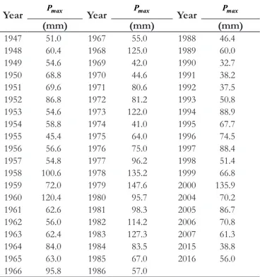
The case study addressed in this section is about the implementation project of bridge in road ES-060, located in the Marataízes municipality, state of Espírito Santo. Table 8 presents data on annual maximum precipitation obtained from the National Water Agency (ANA) regarding the Marataízes station (code 02140000). The drainage basin under consideration has an area of 19.12 km2, a mean declivity of 1%, and a length of the main channel of approximately 9.15 km. The use and occupation of the soil includes pasture lands, urban areas, and water surface.
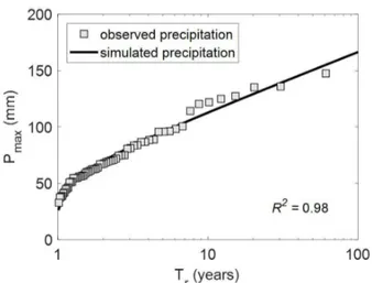
Figure 8 presents the results of the Gumbel model optimization process for the annual maximum precipitation data
observed in the region of Marataízes/ES. Figure 8 also indicates
the value obtained for the coefficient of determination ( 2
R= 0.985).
Figure 9 shows the IDF curves for this case study, referring to three return periods: 5, 25, and 100 years. From the comparison with the calibration data (circles), obtained via daily rainfall Figure 7. Marginal posterior distribution histograms of the parameters a b c, , and d of the IDF model obtained with the DREAM
software.
Table 8. Annual maximum daily precipitations during the period from 1947 to 2016, in Marataízes/ES.
Year Pmax Year Pmax Year Pmax
(mm) (mm) (mm)
1947 51.0 1967 55.0 1988 46.4
1948 60.4 1968 125.0 1989 60.0
1949 54.6 1969 42.0 1990 32.7
1950 68.8 1970 44.6 1991 38.2
1951 69.6 1971 80.6 1992 37.5
1952 86.8 1972 81.2 1993 50.8
1953 54.6 1973 122.0 1994 88.9
1954 58.8 1974 41.0 1995 67.7
1955 45.4 1975 64.0 1996 74.5
1956 56.6 1976 75.0 1997 88.4
1957 54.8 1977 96.2 1998 51.4
1958 100.6 1978 135.2 1999 66.8
1959 72.0 1979 147.6 2000 135.9
1960 120.4 1980 95.7 2004 70.2
1961 62.6 1981 98.3 2005 86.7
1962 56.0 1982 114.2 2006 70.8
1963 62.4 1983 127.3 2007 61.3
1964 84.0 1984 83.5 2015 38.8
1965 63.0 1985 67.0 2016 56.0
disaggregation, and the simulation from the rainfall equation obtained with the optimal parameters, it is possible to observe a reasonable adjustment between the model and the rainfall intensity calibration data.
The heavy rainfall equation estimated using the developed system was the following:
.
. .
.
( . )
0 16
r 0 88
d
1647 42T
i
T 16 01
=
+ (7)
With the data obtained from the rainfall equation, discharges that are widely used in drainage projects, such as roadworks, become easy to estimate. This study also developed a Toolbox that automatically extracts the data from the rainfall equation and calculates the design discharge through the synthetic unit hydrograph method (Toolbox HU). Details about the implementation of this Toolbox are to be presented in a future study, its description is not the goal of this article.
DISCUSSIONS
The system presented in this article enabled the obtainment of the rainfall intensity equation for a certain time series of precipitations. Differential Evolution was used as an algorithm of global optimization to automatically estimate optimal parameters for the Gumbel model, as well as for the IDF curves.
The Gumbel distribution employed in this article as a model for the annual maximum precipitations has a light upper tail, which may underestimate precipitation or discharge values for return periods of larger magnitude. On the other hand, recent studies from the hydrology research community have investigated the adequacy of models with heavy upper tail (KATZ; PARLANGE; NAVEAU, 2002; COSTA; FERNANDES; NAGHETTINI, 2015; LIMA et al., 2016; SILVA et al., 2017; COSTA; FERNANDES, 2017), such as the log-normal distribution. For example, while the log-normal distribution may not have a good adjustment to the precipitation data related to longer return periods, it does shows a better adjustment to the quantiles associated to the return periods of greater magnitude when compared to the Gumbel model. In the developed system, the Anderson-Darling test was incorporated to the program’s output data. With this, the user is able to judge the potential of the Gumbel distribution in the modeling of the annual maximum precipitations, as well as, eventually, adapting the code with the use of a heavy-upper-tailed model. Moreover, the Gumbel distribution is a relatively simple analytical model, and it was employed in the proposed system due to its broad utilization in road projects. However, there is a tendency of using distributions with more parameters in order to describe the skewness and kurtosis characteristics of maximum daily precipitation samples (PAPALEXIOU; KOUTSOYIANNIS, 2016).
The DREAM algorithm was used as benchmark for evaluating the coupled system based on Differential Evolution. The posterior parameter distributions for both models had maximum values that were very close to the ones estimated with the system proposed in this article and described in Figure 1. Furthermore, the adjustment with the calibration data, both for
the Gumbel model and for the IDF curves, confirmed the system’s
potential applications. It is worth mentioning that the employed analytical models are relatively simple, and the search capacity for the global optimum of the Differential Evolution algorithm is strong. In addition, the employed method for daily rainfall disaggregation (Table 4) may not be representative and may possibly generate inconsistencies in the precipitation intensity associated with short durations. Indeed, the model from the Environmental Company of São Paulo State (Companhia Ambiental do Estado de São Paulo - CETESB), despite being frequently used, is over 30 years old, thus being susceptible to further analysis, which is beyond the aim of this study.
CONCLUSIONS
Rainfall intensity equations are widely used in the design of drainage structures for different purposes, including engineering structures in road projects. A precise characterization of rainfall intensity equations is therefore vital for the appropriate sizing of these drainage structures. Thus, a computer system that enables Figure 8. Adjustment of the Gumbel distribution to the annual
maximum precipitations (Pmax) in Marataízes/ES.
the automatized obtainment of the design discharge is of great importance.
This article introduced the different elements of the computer system developed for the automatic adjustment and coupling of the Gumbel model and of the IDF curves for the obtainment of the rainfall intensity equation, without the need of the user providing any prior information about the parameters. In addition, the computer code also provides the design discharge by including additional information about the drainage basin under consideration.
Differential Evolution was used to obtain the optimal parameters of the models. This global optimization technique enables a sweep through search space in order to obtain the parameters that best mimic the calibration data. The objective function employed was the root-mean-square-error (RMSE), which measures the distance between the observed and simulated precipitation values. The performance of the proposed system was tested with Markov chain Monte Carlo simulations using the DREAM software. The results showed that the optimal values for the parameters obtained with the system described in this study demonstrated a good degree of agreement with the results obtained with DREAM.
A practical case study involving the obtainment of the design discharge employed in the design of a special engineering structure was used to illustrate the usability and applicability of the developed system and methodology. The results demonstrated that there was a reasonable adjustment of the Gumbel model (R2=0 985. ), as well as a remarkable agreement between the IDF curve and the rainfall intensity calibration data.
The system presented in this article was specially developed for the utilization in hydrological studies of road projects. From data on annual maximum precipitation, which are easily available online, the computer code is able to generate rainfall equations with accuracy, enabling an annual update of the equation.
ACKNOWLEDGEMENTS
The authors would like to thank two anonymous reviewers for their contributions to the previous versions of this article. Alex Sandro Paulino Gomes is thankful for the support during the data collection and testing of the computer code herein presented. The computer system developed in MATLAB for determining the rainfall equation and for calculating the design discharge in hydrological studies is available upon direct request
to the first author via the e-mail address: guilhermejcg@yahoo.
com.br. This includes the data and scripts used in this article.
REFERENCES
CARDOSO, C. O.; ULLMANN, M. N.; BERTOL, I. Análise de chuvas intensas a partir da desagregação das chuvas diárias de Lages e de Campos Novos (SC). Revista Brasileira de Ciência do Solo, v. 22, n. 1, p. 131-140, 1998. http://dx.doi.org/10.1590/ S0100-06831998000100018.
CETESB – COMPANHIA DE TECNOLOGIA DE SANEAMENTO AMBIENTAL. Drenagem urbana: manual de projeto. São Paulo: CETESB, 1986. 464 p.
CHOW, V. T.; MAIDMENT, D. R.; MAYS, L. W. Applied hydrology. New York: McGraw-Hill, 1988. 564 p.
COSTA, V.; FERNANDES, W. Bayesian estimation of extreme flood quantiles using a rainfall-runoff model and a stochastic daily rainfall generator. Journal of Hydrology, v. 554, p. 137-154, 2017. http://dx.doi.org/10.1016/j.jhydrol.2017.09.003.
COSTA, V.; FERNANDES, W.; NAGHETTINI, M. A Bayesian model for stochastic generation of daily precipitation using an upper-bounded distribution function. Stochastic Environmental Research and Risk Assessment, v. 29, n. 2, p. 563-576, 2015. http:// dx.doi.org/10.1007/s00477-014-0880-9.
DEMIRHAN, H. A generalized Gumbel distribution and its parameter estimation. Communications in Statistics. Simulation and Computation, v. 0, n. 0, p. 1-20, 2017. http://dx.doi.org/10.1080/ 03610918.2017.1361976.
FADHEL, S.; RICO-RAMIREZ, M. A.; HAN, D. Uncertainty of Intensity-Duration-Frequency (IDF) curves due to varied climate baseline periods. Journal of Hydrology, v. 547, p. 600-612, 2017. http://dx.doi.org/10.1016/j.jhydrol.2017.02.013.
GARCIA, S. S.; AMORIM, R. S. S.; COUTO, E. G.; STOPA, W. H. Determinação da equação intensidade-duração-frequência para três estações meteorológicas do Estado de Mato Grosso. Revista Brasileira de Engenharia Agrícola e Ambiental, v. 15, n. 6, p. 575-581, 2011. http://dx.doi.org/10.1590/S1415-43662011000600006.
KANG, M. S.; KOO, J. H.; CHUN, J. A.; HER, Y. G.; PARK, S. W.; YOO, K. A mathematical framework for studying rainfall intensity-duration-frequency relationships. Biosystems Engineering, v. 104, n. 3, p. 425-434, 2009. http://dx.doi.org/10.1016/j. biosystemseng.2009.07.004.
KARAHAN, H. Determining rainfall-intensity-duration-frequency relationship using Particle Swarm Optimization. KSCE Journal of Civil Engineering, v. 16, n. 4, p. 667-675, 2012. http://dx.doi. org/10.1007/s12205-012-1076-9.
KARAHAN, H.; AYVAZ, M. T.; GURARSLAN, G. Determination of intensity-duration-frequency relationship by Genetic Algorithm: case study of GAP. Teknik Dergi, v. 19, n. 2, p. 4393-4407, 2008.
KATZ, R. W.; PARLANGE, M. B.; NAVEAU, P. Statistics of extremes in hydrology. Advances in Water Resources, v. 25, n. 8-12, p. 1287-1304, 2002. http://dx.doi.org/10.1016/S0309-1708(02)00056-8.
KOUTSOYIANNIS, D.; ONOF, C. Rainfall disaggregation using adjusting procedures on Poisson cluster model. Journal of Hydrology, v. 246, n. 1-4, p. 109-122, 2001. http://dx.doi.org/10.1016/ S0022-1694(01)00363-8.
LIMA, C. H. R.; LALL, U.; TROY, T.; DEVINENI, N. A hierarchical Bayesian GEV model for improving local and regional flood quantile estimates. Journal of Hydrology, v. 541, p. 816-823, 2016. http://dx.doi.org/10.1016/j.jhydrol.2016.07.042.
MADSEN, H.; MIKKELSEN, P. S.; ROSBJERG, D.; HARREMOËS, P. Regional estimation of rainfall intensity-duration-frequency curves using generalized least squares regression of partial duration series statistics. Water Resources Research, v. 38, n. 11, p. 21-1-21-11, 2002. http://dx.doi.org/10.1029/2001WR001125.
MOHYMONT, B.; DEMARÉE, G. R.; FAKA, D. N. Establishment of IDF-curves for precipitation in the tropical area of Central Africa – comparison of techniques and results. Natural Hazards and Earth System Sciences, v. 4, n. 3, p. 375-387, 2004. http://dx.doi. org/10.5194/nhess-4-375-2004.
PAPALEXIOU, S. M.; KOUTSOYIANNIS, D. Entropy based derivation of probability distributions: a case study to daily rainfall. Advances in Water Resources, v. 45, p. 51-57, 2012. http://dx.doi. org/10.1016/j.advwatres.2011.11.007.
PAPALEXIOU, S. M.; KOUTSOYIANNIS, D. A global survey on the seasonal variation of the marginal distribution of daily precipitation. Advances in Water Resources, v. 94, p. 131-145, 2016. http://dx.doi.org/10.1016/j.advwatres.2016.05.005.
PAPALEXIOU, S. M.; KOUTSOYIANNIS, D.; MAKROPOULOS, C. How extreme is extreme? An assessment of daily rainfall distribution tails. Hydrology and Earth System Sciences, v. 17, n. 2, p. 851-862, 2013. http://dx.doi.org/10.5194/hess-17-851-2013.
PENNER, G. C.; LIMA, M. P. Comparação entre métodos de determinação da equação de chuvas intensas para a cidade de Ribeirão Preto. Geociências, v. 35, n. 4, p. 542-559, 2016.
SABÓIA, M. A. M.; SOUZA FILHO, F. A.; ARAUJO JUNIOR, L. M.; SILVEIRA, C. S. Climate changes impact estimation on urban drainage system located in low latitudes districts: a study case in Fortaleza-CE. Revista Brasileira de Recursos Hídricos, v. 22, n. 21, 2017. http://dx.doi.org/10.1590/2318-0331.011716074.
SILVA, A. T.; PORTELA, M. M.; NAGHETTINI, M.; FERNANDES, W. A Bayesian peaks-over-threshold analysis of floods in the
Itajaí-açu River under stationarity and nonstationarity. Stochastic Environmental Research and Risk Assessment, v. 31, n. 1, p. 185-204, 2017. http://dx.doi.org/10.1007/s00477-015-1184-4.
SILVA, B. M.; MONTENEGRO, S. M. G. L.; SILVA, F. B.; ARAUJO FILHO, P. F. Chuvas Intensas em Localidades do Estado de Pernambuco. Revista Brasileira de Recursos Hídricos, v. 17, n. 3, p. 135-147, 2012. http://dx.doi.org/10.21168/rbrh.v17n3.p135-147.
STORN, R.; PRICE, K. Differential evolution: a simple and efficient heuristic for global optimization over continuous spaces. Journal of Global Optimization, v. 11, n. 4, p. 341-359, 1997. http:// dx.doi.org/10.1023/A:1008202821328.
TUCCI, C. E. M. Hidrologia ciência e aplicação. Porto Alegre: ABRH, 1993. 943 p.
VIVEKANANDAN, N. Prediction of seasonal and annual rainfall using order statistics approach of Gumbel and freshet distributions. Journal of Civil Engineering and Urbanism, v. 7, n. 1, p. 12-17, 2017.
VRUGT, J. A. Markov chain Monte Carlo simulation using the DREAM software package: theory, concepts, and MATLAB implementation. Environmental Modelling & Software, v. 75, p. 273-316, 2016. http://dx.doi.org/10.1016/j.envsoft.2015.08.013.
VRUGT, J. A.; BEVEN, K. Embracing equifinality with efficiency: Limits of Acceptability sampling using the DREAM(LOA) algorithm. Journal of Hydrology, v. 559, p. 954-971, 2018. http:// dx.doi.org/10.1016/j.jhydrol.2018.02.026.
WRIGHT, D. B.; SMITH, J. A.; BAECK, M. L. Flood frequency analysis using radar rainfall fields and stochastic storm transposition. Water Resources Research, v. 50, n. 2, p. 1592-1615, 2014. http:// dx.doi.org/10.1002/2013WR014224.
Authors contributions
Guilherme José Cunha Gomes: Bibliographic research, data collection and treatment, computer code development, analysis of the results and elaboration of the text.
Eurípedes do Amaral Vargas Júnior: Guidance of the study,
contribution in the definition and interpretation of the methodology,