www.atmos-chem-phys.net/17/501/2017/ doi:10.5194/acp-17-501-2017
© Author(s) 2017. CC Attribution 3.0 License.
Quantifying the volatility of organic aerosol in the southeastern US
Provat K. Saha1, Andrey Khlystov2, Khairunnisa Yahya3, Yang Zhang3, Lu Xu4, Nga L. Ng4,5, and Andrew P. Grieshop1
1Department of Civil, Construction and Environmental Engineering, North Carolina State University, Raleigh, NC, USA 2Division of Atmospheric Sciences, Desert Research Institute, Reno, Nevada, USA
3Department of Marine Earth and Atmospheric Sciences, North Carolina State University, Raleigh, NC, USA 4School of Chemical and Biomolecular Engineering, Georgia Institute of Technology, Atlanta, GA, USA 5School of Earth and Atmospheric Sciences, Georgia Institute of Technology, Atlanta, GA, USA
Correspondence to:Andrew P. Grieshop ([email protected])
Received: 3 July 2016 – Published in Atmos. Chem. Phys. Discuss.: 9 August 2016 Revised: 17 November 2016 – Accepted: 7 December 2016 – Published: 11 January 2017
Abstract. The volatility of organic aerosols (OA) has emerged as a property of primary importance in understand-ing their atmospheric life cycle, and thus abundance and transport. However, quantitative estimates of the thermody-namic (volatility, water solubility) and kinetic parameters dictating ambient-OA gas-particle partitioning, such as satu-ration concentsatu-rations (C∗), enthalpy of evaporation (1H
vap),
and evaporation coefficient (γe), are highly uncertain. Here,
we present measurements of ambient-OA volatility at two sites in the southeastern US, one at a rural setting in Al-abama dominated by biogenic volatile organic compounds (BVOCs) as part of the Southern Oxidant and Aerosol Study (SOAS) in June–July 2013, and another at a more anthro-pogenically influenced urban location in North Carolina dur-ing October–November 2013. These measurements applied a dual-thermodenuder (TD) system, in which temperature and residence times are varied in parallel to constrain equilibrium and kinetic aerosol volatility properties. Gas-particle parti-tioning parameters were determined via evaporation kinetic model fits to the dual-TD observations. OA volatility param-eter values derived from both datasets were similar despite the fact that measurements were collected in distinct settings and seasons. The OA volatility distributions also did not vary dramatically over the campaign period or strongly correlate with OA components identified via positive matrix factoriza-tion of aerosol mass spectrometer data. A large porfactoriza-tion (40– 70 %) of measured ambient OA at both sites was composed of very-low-volatility organics (C∗≤0.1 µg m−3). An
effec-tive1Hvapof bulk OA of∼80–100 kJ mol−1and aγevalue
of ∼0.5 best describe the evaporation observed in the TDs.
This range of1Hvapvalues is substantially higher than that
typically assumed for simulating OA in atmospheric models (30–40 kJ mol−1). TD data indicate thatγ
eis on the order of
0.1 to 0.5, indicating that repartitioning timescales for atmo-spheric OA are on the order of several minutes to an hour un-der atmospheric conditions. The OA volatility distributions resulting from fits were compared to those simulated in the Weather, Research and Forecasting model with Chemistry (WRF/Chem) with a current treatment of secondary organic aerosol (SOA) formation. The substantial fraction of low-volatility material observed in our measurements is largely missing from simulations, and OA mass concentrations are underestimated. The large discrepancies between simulations and observations indicate a need to treat low-volatility OA in atmospheric models. Volatility parameters extracted from ambient measurements enable evaluation of emerging treat-ments for OA (e.g., secondary OA using the volatility basis set or formed via aqueous chemistry) in atmospheric models.
1 Introduction
oxi-dation reactions of gas-phase organic species; it may also be formed by reactions in the particle (condensed) phase (Kroll and Seinfeld, 2008). A large fraction of SOA in many parts of the globe, e.g., in the southeastern US, is formed from biogenic volatile organic compounds (BVOCs) (Goldstein et al., 2009; Goldstein and Galbally, 2007). However, the mechanisms responsible for SOA production from BVOCs (Budisulistiorini et al., 2015; Goldstein and Galbally, 2007; Marais et al., 2016; Xu et al., 2015a, b), its chemical com-position, and many important physical properties are largely undetermined (Goldstein et al., 2009; Schichtel et al., 2008; Weber et al., 2007). Therefore, their representation in current atmospheric and climate models are highly uncertain (Hal-lquist et al., 2009; Liao et al., 2007; Pye et al., 2015; Pye and Seinfeld, 2010).
One of the major sources of uncertainty in predicting SOA concentrations in atmospheric models arises from the poor understanding of gas-particle partitioning of chemical species comprising SOA (Hallquist et al., 2009; Jimenez et al., 2009; Seinfeld and Pankow, 2003). Gas-particle parti-tioning plays a central role in determining life cycle of OA and thus its atmospheric abundance, transport, and impacts (Donahue et al., 2006; Jimenez et al., 2009). At equilibrium, the volatility of organic species, specifically saturation va-por pressure (or equivalently, saturation concentration, C∗; µg m−3), plays a vital role in determining their gas-particle
partitioning. (Donahue et al., 2006; Pankow, 1994). Solu-bility of organic species in water may also be critical for gas-particle partitioning for many species (Hennigan et al., 2009), especially in places with higher relative humidity, in the southeastern US, for example. Enthalpies of vaporiza-tion (1Hvap)dictate the change in partitioning with temper-ature (Donahue et al., 2006; Epstein et al., 2010). Although gas-particle partitioning is determined by the basic thermo-dynamic properties of OA species – their C∗,1Hvap, and
solubility – these, along with the impacts of nonideal mix-ing on individual species, are generally unknown for ambient OA. Under changing conditions, gas-particle partitioning is also influenced by the kinetics of gas-particle exchange, for example due to barriers to mass transfer in solid or viscous particles or molecular accommodation at a particle surface (Kroll and Seinfeld, 2008). The overall kinetic limitation to mass transfer during repartitioning is typically described by an evaporation coefficient (γe) (also often called mass ac-commodation coefficient), which is highly uncertain for am-bient OA and can dictate timescales for partitioning (Saleh et al., 2013). Though current models assume OA to be at equi-librium within a model prediction time step (several minutes to an hour) during atmospheric simulations, several studies have indicated that partitioning timescales could be as long as days or months (γe≪0.1) due to a highly viscous and/or
glassy aerosol (Vaden et al., 2011; Zobrist et al., 2008). Quantitative measures of ambient-OA gas-particle parti-tioning parameters are needed to provide inputs for, and to evaluate, atmospheric models. However, methods to
quan-titatively determine ambient-OA volatility are in their in-fancy and the resulting estimates of parameters dictating OA volatility are highly uncertain (Cappa and Jimenez, 2010). Thermodenuder (TD) systems have been previously applied to measure ambient-OA volatility (Burtscher et al., 2001; Huffman et al., 2009; Lee et al., 2010; Paciga et al., 2016; Xu et al., 2016). A TD system measures evaporation of sam-pled aerosol at various temperature perturbations by system-atically comparing the size distribution and/or aerosol mass concentration measured after heating in a TD and at a ref-erence (“bypass”) condition (Huffman et al., 2008). Several efforts have been made to infer ambient-OA volatility dis-tributions by fitting observed evaporation in a TD using a model of evaporation kinetics (Cappa and Jimenez, 2010; Lee et al., 2010). However, since OA evaporation in a TD is dictated by a large number of independent parameters (e.g., C∗,1H
vap, andγe)(Cappa and Jimenez, 2010; Lee et al., 2010), it is difficult to constrain all parameters with a one-dimensional perturbation (e.g., varying TD temperature) to the initial equilibrium. Saha et al. (2015) showed that oper-ating two TDs in parallel (dual-TD), varying both temper-ature and residence time, can provide tighter constraint on estimates of volatility parameter values (C∗,1H
vap, andγe) for single-component OA via kinetic model fits to the obser-vations. In Saha and Grieshop (2016), this approach was ap-plied to determine volatility and phase-partitioning parame-ter values for laboratoryα-pinene SOA. The resulting param-eters are consistent with recent observations of low-volatility SOA (Jokinen et al., 2015; Zhang et al., 2015) and evapora-tion rates (Vaden et al., 2011; Wilson et al., 2015) observed by several techniques. TD perturbations alone cannot give in-sights into the solubility of OA components, though they may be used to do so in concert with other techniques (Cerully et al., 2015).
This paper describes the application of the dual-TD ap-proach during ambient observations from two different set-tings in the southeastern US. Measurements at a rural site during the Southern Oxidant and Aerosol Study (SOAS-2013) (https://soas2013.rutgers.edu/) leverage the range of complementary measurements available during this large field study. To provide a contrast, measurements were also taken several months later under cooler conditions in Raleigh, US, a small metropolitan area in a similar ecologi-cal zone but with stronger influence from loecologi-cal anthropogenic emissions. The objectives of the study were to (i) determine a set of volatility parameter values, such as OA volatility distribution using the volatility basis set (VBS) framework (Donahue et al., 2006, 2012),1Hvap, and γe, that describe
with that simulated by a chemical transport model using a current implementation of the VBS framework.
2 Methods
2.1 Measurement sites
Ambient OA volatility measurements were conducted at two locations in the southeastern US, one in a forested rural set-ting and another in an urban location. During the Southern Oxidant and Aerosol Study (SOAS-2013) field campaign, 6 weeks (1 June to 15 July 2013) of continuous measure-ments were conducted in rural Alabama. The SOAS field campaign occurred in summer 2013 at several locations in the southeastern US in order to study the interaction of bio-genic and anthropobio-genic atmospheric compounds with a fo-cus on BVOCs and organic aerosols. The measurements re-ported here are from the main SOAS ground site (32.903◦N,
87.250◦W) near Talladega National Forest and Centreville,
Alabama. The Centreville, Alabama, site is an ideal location to study volatility of OA dominated by secondary OA from BVOC precursors (Warneke et al., 2010) in the presence of a range of anthropogenic influences. An additional 4 weeks (18 October to 20 November 2013) of ambient-OA volatility measurements were conducted at the North Carolina State University (NCSU) main campus (35.786◦N, 78.669◦W) in
Raleigh, US. The NCSU site, while in an area with plenti-ful tree cover and BVOC emissions, receives a substantially stronger influence from anthropogenic emissions due to its location within the Raleigh metro area. Section 3.1 includes further comparison between two study areas. Hereafter, the two datasets are referred to as Centreville and Raleigh.
2.2 Dual-thermodenuder operation and sampling strategy
Measurements were collected using the dual-TD experimen-tal setup introduced in Saha et al. (2015) and are only briefly described here. Two TDs operated in parallel, one at various temperature settings (temperature stepping TD, TS-TD) with a fixed, relatively longer residence time (Rt) and another at fixed temperature and various Rt settings (variable residence time TD, VRT-TD). The TS-TD temperature settings were 40, 60, 90, 120, 150, and 180◦with∼50 s Rt, while the
VRT-TD operated at 60 or 90◦with Rt varying between 1 and 40 s
(five to eight settings). All Rts reported here are calculated assuming plug flow at room temperature. Temperature ef-fects on Rt were included during modeling of evaporation ki-netics (discussed below) as Rt (TTD)=Rt(Tref)×(Tref/TTD),
whereTrefandTTDare the reference temperatures (e.g., room
temperature) and TD temperature in K, respectively (Cappa, 2010). The time to run through all temperatures and Rt steps during measurements was∼4–5 h.
A schematic of the experimental setup is shown in Fig. 1. Three scanning mobility particle sizers (SMPS, TSI Inc,
Ambient air PM2.5inlet
TS-TD: Rt=50 s
VRT-TD: Rt=1–40 s
Di
ff
usio
n
dr
y
er
T/RH
Automated three-way valve
SMPS-3 ACSM
Bypass EFC
SMPS-2 SMPS-1
pr
obe
Inside trailer
T = 60/90 deg C
T = 40 – 180 deg C
Figure 1. Dual-thermodenuder aerosol volatility measurement setup used during field campaigns at two sites in the southeast-ern US. TS-TD: temperature stepping TD, VRT-TD: variable resi-dence time TD, Rt: resiresi-dence time, EFC: extra flow control, ACSM: aerosol chemical speciation monitor, SMPS: scanning mobility par-ticle sizer.
Model 3081 DMAs, Model 3010/3787 CPCs) simultane-ously measured aerosol size distributions (10–600 nm) in three parallel lines (two TDs and one bypass). An aerosol chemical speciation monitor (ACSM, Aerodyne Research Inc.) alternated between the bypass and TS-TD lines at∼20–
30 min intervals using an automated three-way valve system. The ACSM measured the submicron aerosol (∼75–650 nm)
mass concentration of nonrefractory chemical species (or-ganic, sulfate, nitrate, ammonium, and chloride) (Ng et al., 2011a).
All aerosol instruments and TD inlets were inside a temperature-controlled (25◦C±2) trailer in Centreville and
laboratory room in Raleigh. Ambient air was continuously sampled through a sampling inlet located on the rooftop of a trailer or building (∼5 m above ground level). The sampling
inlet included a PM2.5 cyclone (URG Corp, 16.7 L min−1) followed by an∼8 mm inner diameter copper sample line. A
silica gel diffusion dryer upstream of TD inlets and aerosol instruments maintained relative humidity (RH) < 30–40 %. The dryer is required for instrument operation under hu-mid ambient conditions but may induce some loss of water-soluble OA components (El-Sayed et al., 2016).
2.3 Quantifying OA evaporation
quantita-tive assessment of aerosol volatility, such as during modeling of aerosol evaporation, the initial OA concentration (COA) and particle size are also needed. Empirically estimated par-ticle loss correction factors as a function of TD tempera-tures and residence times (Saha et al., 2015) and instrumental inter-calibration factors were applied in MFR calculations. To get directly comparable SMPS concentration data from three SMPSs running in parallel with our dual-TD system, we ran them periodically in parallel on the bypass line to de-termine intercalibration factors. Further details on SMPS in-tercomparison are discussed in Saha et al. (2015). Since the VRT-TD line was only measured with the SMPS (Fig. 1), it only provided information on evaporation of submicron aerosol in terms of its volume concentration. We estimated the OA MFR from VRT-TD and SMPS data assuming mea-sured aerosol volume was only comprised of OA and am-monium sulfate (AS). This is a reasonable assumption un-der these conditions because more than 90 % of measured aerosol volume concentrations can be explained by OA+AS
for both sites (see Supplement, Fig. S1). Our calculations also assumed that AS did not evaporate at the VRT-TD oper-ating temperatures (60 or 90◦C) (Fig. S2). For further details
on the estimation of approximate OA MFR from VRT-TD and SMPS data, see Sect. S1.
2.4 Determining OA gas-particle partitioning parameters
We apply a previously described volatility parameter extrac-tion framework (Saha et al., 2015; Saha and Grieshop, 2016) to extract a set of volatility parameter (C∗,1H
vap,γe)
val-ues via inversion of dual-TD data using an evaporation ki-netics model. The evaporation kiki-netics model used here is that described in Lee et al. (2011). The approach is briefly outlined below. The resulting fit describes OA using a log10
volatility basis set (VBS) framework (Donahue et al., 2006, 2012), where material is lumped into volatility bins separated by orders of magnitude inC∗space at a reference tempera-ture (Tref). The volatility distribution extracted using this
ap-proach is an empirical estimate describing the bulk volatility behavior of OA, assuming absorptive partitioning (Donahue et al., 2006, 2012). The VBS approach is based on an ef-fective saturation concentration (C∗) where the activity
co-efficient is assumed to be lumped into the saturation concen-tration. In the VBS approach, total OA concentration (COA;
µg m−3)is modeled using Eq. (1).
COA=CtotX i
fi
1+ C ∗
i COA
−1
(1)
Here, Ctot is the total organic material (vapor+aerosol) in
phase equilibrium withCOAandfi is the fraction ofCtotin
each volatility (log10C∗)bin. Thus,fi=Ctot,i/Ctotdescribes
the distribution of organics in volatility space and is usually called the volatility distribution.
The Clausius–Clapyeron equation (Eq. 2) is used to repre-sent temperature-dependentC∗.
Ci∗(T )=Ci∗(Tref)exp
−1Hvap,i
R
1
T − 1 Tref
T
ref
T , (2) whereR is the gas constant and1Hvap is the enthalpy of
vaporization.
To extract the volatility distribution of OA from ambi-ent measuremambi-ents, we select lower- and upper-C∗ (T
ref) bins of 10−4and 101µg m−3, respectively. A reference
tem-perature (Tref) of 298 K is assumed. All C∗ values re-ported in this paper should be considered at 298 K, unless otherwise specified. The selection of the lower and upper bins are determined by the highest TD operating tempera-ture (180◦C) and the average ambient-OA loading (C
OA∼
5 µg m−3), respectively. With theseC∗ bin limits, materials
withC∗< 10−4µg m−3are lumped into the lowest bin, while
materials withC∗> 10 µg m−3are not represented. Note, if a C∗bin of 100 µg m−3is included, Eq. (1) indicates that less than 5 % of the material in this bin will be in the condensed phase at COA∼5 µg m−3. Therefore, C∗ bins > 10 µg m−3 are not well constrained by our TD data and are not included in our analysis.
The general approach to fitting a volatility parameteriza-tion employed in this study is similar to that applied to labo-ratory aerosol systems (Saha et al., 2015; Saha and Grieshop, 2016). Briefly, the kinetic model tracks both particle- and gas-phase concentrations of model species (each represented by a VBS bin) as they proceed through TD operated at a particular temperature and residence time. The model takes inputs of several aerosol properties (e.g., C∗ distribution,
1Hvap, diffusion coefficient (D), surface tension (σ ),
molec-ular weight (MW), and density (ρ)), total aerosol loading (COA), and particle diameter (dp)and determines how much aerosol mass concentration will evaporate for a set of in-put parameters at a particular TD temperature and residence time. Non-continuum effects on mass transfer are repre-sented using the Fuchs–Sutugin correction factor, which de-pends onγe. The model is applied to extract OA properties
such as the volatility distribution, 1Hvap, and γe as fitting
parameters by matching measured and modeled evaporation data. Values ofD,σ, MW, andρgenerally have a smaller in-fluence on observed evaporation (Cappa and Jimenez, 2010; Saha et al., 2015) and are approximated from literature val-ues (Table S1). Volume median diameter was used as a rep-resentative dp. For simplicity, a large (1Hvap, γe) space was considered for fitting afi distribution of measured OA. Following previous work (Epstein et al., 2010; May et al., 2013), a linear relationship was assumed between1Hvapand
log10C∗with1Hvap,i=intercept-slope (log10Ci,∗298), where intercept and slope are fit parameters. Values for 1Hvap
intercept=[50, 80, 100, 130, 200] and slope=[0, 4, 8,
11] kJ mol−1were applied along withγ
e=[0.01, 0.05, 0.1,
effective parameter representing all kinetic limitations within the condensed phase and at the particle surface.
A distribution of fi was solved for each combination of (1Hvap,γe)applying the nonlinear constrained optimization solver “fmincon” in MATLAB (Mathworks, Inc.) by first
fit-ting TS-TD data; accepted solutions were then further refined by fitting VRT-TD observations. A constraint of6fi=1 was used. The goodness of fit was quantified in terms of the sum of squared residual (SSR) values. For the campaign-average fit, an acceptance threshold value for SSR was selected based on observed variability (±one standard deviation) in
mea-surements. A parameter set (fi, 1Hvap, and γe)was con-sidered a finally accepted solution if it optimally reproduced both TS-TD and VRT-TD observations within the observed variability. Raw data at each (T, Rt) condition were averaged over 20–30 min. At given TD operating conditions (T, Rt), we defined±1 standard deviation of MFR data (20–30 min
resolution) from the whole campaign as an indicator of the observed variability. The best fit is defined as that with the lowest SSR value among all the accepted combinations.
2.5 Simulation of OA in a chemical transport model Considering that VBS-based parameterizations are becom-ing common means to improve the performance of OA pre-diction in chemical transport models (CTMs) (Farina et al., 2010; Lane et al., 2008b; Matsui et al., 2014; Murphy et al., 2011; Shrivastava et al., 2013), measurements of OA volatil-ity provide a useful means by which to evaluate these sim-ulations. We compared OA volatility distributions measured in this study to those resulting from CTM simulations us-ing a current VBS-based parameterization implemented in a modified version of the Weather, Research and Forecast-ing model with Chemistry (WRF/Chem) v3.6.1 (Wang et al., 2015; Yahya et al., 2016). The WRF/Chem simulation uses the Carbon Bond version 6 (CB6) gas-phase mecha-nism (Yarwood et al., 2010) coupled by Wang et al. (2015) to the Model for Aerosol Dynamics for Europe – Volatility Basis Set (MADE/VBS) (Ackermann et al., 1998; Ahmadov et al., 2012; Shrivastava et al., 2011). The CB6-MADE/VBS treatment includes semivolatile POA and SOA, as well as a fragmentation and functionalization treatment for multigen-erational OA aging based on Shrivastava et al. (2013). The fragmentation and functionalization treatment in this case as-sumes 25 % fragmentation for the third and higher genera-tions of oxidation (Shrivastava et al., 2013). The ranges of C∗values used in WRF/Chem simulation are defined based
on current SOA and semivolatile POA parameterizations and were 100 to 103µg m−3 for ASOA (anthropogenic SOA)
and BSOA (biogenic SOA), 10−2 to 106µg m−3 for POA
and 10−2to 105µg m−3for SVOA (semivolatile OA), where
SVOA refers to oxidized OA from evaporated POA. The semiempirical correlation for1Hvapby Epstein et al. (2010)
was used to estimate temperature-dependent partitioning.
The simulations are performed at a horizontal resolution of 36 km with 148×112 horizontal grid cells over the
continen-tal US domain and parts of Canada and Mexico and a vertical resolution of 34 layers from the surface to 100 hPa. Anthro-pogenic emissions in 2010 were based on the 2008 National Emissions Inventory (NEI) from the Air Quality Model Eval-uation International Initiative (AQMEII) project (Pouliot et al., 2015). Biogenic emissions are simulated online by the Model of Emissions of Gases and Aerosols from Nature v2.1 (MEGAN2.1) (Guenther et al., 2012). The chemical initial and boundary conditions (ICs and BCs) come from the mod-ified Community Earth System Model/Community Atmo-sphere Model (CESM/CAM v5.3) with updates by He and Zhang (2014) and Gantt et al. (2014). The meteorological ICs and BCs come from the National Center for Environmental Protection Final Analysis (FNL) data.
3 Results
3.1 Overview of campaign characteristics
The two field campaigns were conducted in settings with distinct local emission sources and metrological conditions. The Centreville campaign was during summer (T =24.7±
3.3◦C, RH=83.1±15.3 %). Local organic emissions
sur-rounding the Centreville site are dominated by BVOCs since this site is located in a forest and biogenic emissions substantially increase with temperature (Lappalainen et al., 2009; Tarvainen et al., 2005; Warneke et al., 2010). In con-trast, Raleigh measurements were in a setting with substan-tially stronger anthropogenic emissions during fall and win-ter (T =12.7±6.0◦C, RH=65.7±18.8 %). Comparison of
long-term data from an air quality monitoring station near the Raleigh site shows substantially higher NOx(5–10-fold) and CO (2–4-fold) concentrations relative to those observed at Centreville (see Fig. S3). However, the Raleigh–Durham metropolitan area has plentiful tree cover and thus substan-tial local BVOC emissions. For instance,α- and β-pinene concentrations measured in summer at Centreville and Duke Forest (about 40 km northwest of the Raleigh site) are in the same range (Fig. S4). However, since the Raleigh cam-paign was conducted at lower temperature conditions, local BVOC emissions are expected to be lower by a factor of 3 to 4 (Fig. S4). Measurements in such diverse but similar eco-logical settings allow us to examine the consistency of OA volatility under varying levels of biogenic and anthropogenic influence.
Figures S5–S7 show average meteorological conditions, submicron aerosol size distributions, chemical composi-tion, and their temporal variations over the campaign pe-riods. Ambient submicron particle number concentrations (10–600 nm) were higher in Raleigh (Centreville: 1500– 3000 cm−3, Raleigh: 3000–6000 cm−3) and particle size
Centre-ville: 275±30 nm, Raleigh: 227±34 nm) (Fig. S6). Organic
species were the dominant component in nonrefractory sub-micron aerosol (PM1) as measured by the ACSM at both sites (Centreville: 71±10 %, Raleigh: 76±8 %). The
cam-paign average±1 standard deviation of ACSM-derived OA
mass concentrations was 5.2±3.0 µg m−3in Centreville and
6.7±3.6 µg m−3in the Raleigh campaign, assuming a
col-lection efficiency (CE) of 0.5. After applying the coarse tracer (m/z)-based factor analysis approach to decompose OA mass spectra (Ng et al., 2011b), the majority of OA measured at both sites was oxygenated OA (OOA). While approximately 7 % of campaign-averaged OA mass concen-tration in Raleigh was classified as hydrocarbon-like OA (HOA), the HOA contribution at the Centreville site was negligible. Positive matrix factorization (PMF) results from high-resolution mass spectra collected at the Centreville site (Xu et al., 2015a, b) and their linkage with the measured OA volatility are discussed in Sect. 3.3 and 3.4 below.
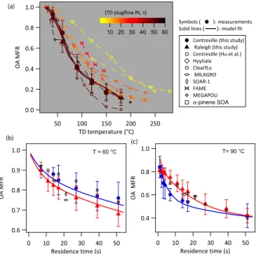
3.2 Observed campaign-average evaporation of OA Figure 2 shows the campaign-average OA MFR as a func-tion of TD temperature and residence time. (1-MFR) at a TD temperature and residence time indicates what fraction of bulk OA mass evaporates at that condition. It is important to note that MFR at a given temperature is not a consistent descriptor of OA volatility because it depends on many pa-rameters related to TD experimental conditions (e.g., Rt) and sampled aerosol (e.g.,COA,dp). Therefore, MFR data should
not be interpreted as a direct measure of OA volatility or even directly compared (unless experiments are conducted under identical conditions).
Figure 2a (MFR vs. temperature, frequently called a ther-mogram plot) shows TS-TD measurements from this study along with one other measurement from SOAS (Hu et al., 2016) and several previous field and laboratory measure-ments. The campaign-average OA MFRs measured at the two sites in the southeastern US, under relatively consis-tent COA∼5 µg m−3, were found to be quite similar.
Ap-proximately 60–70 % of OA mass evaporated after heat-ing at 100◦C with a residence time of 50 s. The
campaign-average T50 and T90 (temperature at which 50 and 90 %
of OA mass evaporates, respectively) with a residence time of 50 s were ∼78 and∼180◦C, respectively. Data from
α-pinene chamber SOA experiments collected using the same dual-TD setup at atmospheric conditions (dark ozonolysis, COA∼5 µg m−3), described in Saha and Grieshop (2016),
are also shown. Relative to the ambient observations, the lab SOA data show similar evaporation behavior in the lower temperature range (40–90◦C) but relatively greater
evapo-ration at higher temperatures.
Figure 2b and c show the campaign-average-estimated OA MFRs at various residence times with the VRT-TD operated at 60 and 90◦C, respectively. Results show increased
evapo-ration with longer residence time. In Fig. 2a, data are color
T = 60 °C T= 90 °C
60 50 40 30 20 10
α-pinene SOA
(a)
(b)
(c)
Figure 2. Measured (solid symbols) and modeled (solid, thick lines) campaign-average organic aerosol (OA) mass fraction re-maining (MFR) as a function of TD temperatures (T) and res-idence times (Rt). The solid symbol shows mean value and the error bar is ± one standard deviation of all campaign data at each (T, Rt) condition. Model lines are shown using the best fit volatility parameter values from campaign-average TD data fit (parameter values listed in Table 1). TD measurement data from the Centreville site collected by the University of Colorado group at SOAS-2013 (Hu et al., 2016) are also shown. Mea-surements from several previous field studies are shown with various open symbols: Hyytiala/2008–2010, Finland (Häkkinen et al., 2012); ClearfLo/2012, London (Xu et al., 2016); MILA-GRO/2006, Mexico City (Huffman et al., 2009); SOAR-1/2005, Riverside, California (Huffman et al., 2009); FAME/2008, Fi-nokalia, Greece (Lee et al., 2010); MEGAPOLI/2009–2010, Paris, France (Paciga et al., 2016). Chamberα-pinene SOA (dark ozonoly-sis,COA∼5 µg m−3, VMD∼140 nm) evaporation data are shown from Saha and Grieshop (2016). In panel(a), data are color coded by TD residence times used during measurements. The legend shown next to panel(a)applies to all panels(a–c).
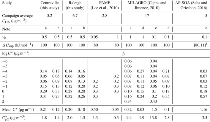
Table 1.Best fit OA volatility parameter values extracted from this study along with several previous field and lab studies.
Study Centreville Raleigh FAME MILAGRO (Cappa and AP-SOA (Saha and
(this study) (this study) (Lee et al., 2010) Jimenez, 2010) Grieshop, 2016)
Campaign average 5.2 6.7 2.8 17 5
COA(µg m−3)
Note a b a b c d c d e
γe 0.5 0.5 0.5 0.5 0.05 1 1 1 0.1 0.1 0.1
1Hvap(kJ mol−1) 100 100 100 100 80 80 100 100 100 100 [80,11]f
logC∗(µg m−3) fi
−6 0.06 0.04
−5 0.06 0.04
−4 0.14 0.18 0.14 0.16 0.06 0.27 0.04 0.21 0.03
−3 0.05 0.05 0.06 0.05 0.2 0.07 0.11 0.04 0.07 0.07
−2 0.06 0.08 0.08 0.13 0.2 0.2 0.07 0.11 0.05 0.09 0.03
−1 0.15 0.13 0.12 0.20 0.2 0.3 0.08 0.12 0.06 0.10 0.12
0 0.29 0.33 0.28 0.20 0.3 0.3 0.10 0.15 0.1 0.18 0.18
1 0.31 0.23 0.32 0.26 0.3 0.16 0.24 0.2 0.35 0.57
2 0.34 0.43
MeanC∗(µg m−3) 0.21 0.12 0.20 0.10 0.50 0.05 0.32 0.03 1.5 0.1 1.16
Ceff∗ (µg m−3) 1.8 1.4 2.0 1.5 1.3 0.3 9.4 1.9 13.8 2.8 3.5
aCampaign-average dual-TD data fit with campaign-averageC OAanddp.
bUnified fit of individual measurements from whole campaign (MFR,C
OA,dp; 20–30 min resolution data). cThef
idistribution derived fromCi,tot=a1+a2exp[a3(log(C∗)−3)];fi=Ci,tot/6Ci,tot;a1,a2, anda3coefficients were taken from Table 1 of Cappa and Jimenez (2010). log10C∗bin ranged from−6 to+2, as in Cappa and Jimenez (2010).
dSame asc, but only considered log10C∗bin range of−4 to+1 to be consistent with the bin ranges used in this study. To do so, materials in log10C∗<−4 bins are
assigned to−4 bin, material at log10C∗=2bin is excluded, and distribution is renormalized to make6f i=1.
eChamber-generated SOA from low-C
OAα-pinene ozonolysis experiment applying renormalization approach described in note d to the distribution given in Saha and Grieshop (2016) Supplement, Table S5.
f1Hvap(kJ mol−1)=80−11logC∗(µg m−3).
the gas phase across the volatility range). The equilibration time of aerosol in a TD is dictated by many parameters, in-cluding particle size distribution, diffusion coefficient (D), and evaporation coefficient (γe)and is typically several min-utes or more under atmospheric (lowCOA)conditions (Saleh et al., 2011, 2013).
Following the method of Saleh et al. (2013), the estimated characteristic equilibration times for the sampled aerosol in the Centreville and Raleigh measurements are 147–470 and 150–450 s, respectively, assuming unhindered mass transfer (γe=1). These calculations are based on the interquartile
ranges of particle number concentrations (Np)and condensa-tion sink diameter (dcs)measured in Centreville (Np∼1500–
3000 cm−3, d
cs∼125–170 nm) and Raleigh (Np∼3000–
6000 cm−3, d
cs∼80–105 nm), and D=3.5×10⁻⁶m2s−1
and MW=200 g mol−1. The condensation sink diameter
(dcs)is estimated following Lehtinen et al. (2003); further detail is given in the Supplement. A factor-of-10 reduction in γerelative to ideal accommodation (γe=0.1) increases
equi-libration time by 1 order of magnitude. The observed contin-uous downward slope of MFR vs. residence time (Fig. 2b, c) suggests that equilibrium was not reached in the TD
dur-ing the maximum Rt of 50 s. This result implies that TD measurements in an ambient setting are essentially a mea-sure of the evaporation rate of sampled aerosol, rather than one of volatility, an equilibrium thermodynamic property. Therefore, an evaporation kinetic model is needed to extract volatility parameter values from ambient TD data.
3.3 Extracted OA volatility parameter values
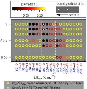
Figure 3 presents the results of the extraction process used to determine parameters dictating gas-particle partitioning (fi, 1Hvap, γe); the example shown is for a fit to the
Centre-ville campaign-average data, though the same process was conducted for all fits. Figure S8 shows a similar plot for the Raleigh dataset. Fitting results show that a broad range of γe (0.05 to 1) can reproduce the TS-TD observation within
observed variability (i.e., error bars in Fig. 2) for several 1Hvap combinations (accepted TS-TD fits are shown with
γe
∆Hvap
γ ∆Hvap
B
Figure 3.Extraction process of OA gas-particle partitioning param-eter (1Hvap,γe andfi)values. Afi distribution was solved for
each combination of (1Hvap,γe)via evaporation kinetic model fits to campaign-average dual-TD observations during the Centreville campaign. A relationship of1Hvap=intercept–slope (log10C∗@ 298 K) was assumed (e.g., 50–0 onxaxis represents intercept=50 and slope=0). Symbols and colors represent the goodness of fit. Points with filled inner circles recreate TS-TD observations and points with a white cross (x) recreate both TD datasets to within observational variability. Crosses represent the overall goodness of fit including both TS-TD and VRT-TD observations, with larger size corresponding to a better fit.
help to narrow the possible solution space. Figure 3 shows that1Hvap=100 kJ mol−1andγe=0.5 provide the overall
best fit for the Centreville dataset. For the Raleigh dataset, 1Hvapof both 80 (marginally better) and 100 kJ mol−1with
γe=0.5 provide similarly good fits (Fig. S8). For simplicity,
1Hvap=100 kJ mol−1 andγe=0.5 are considered as best
estimates for both datasets for the next portion of the paper. These results are inconsistent with a very small value of OA evaporation coefficient (e.g.,γe≪0.1) that would
indi-cate significant resistance to mass transfer during evapora-tion, which has been previously suggested based on dilution (Grieshop et al., 2007, 2009; Vaden et al., 2011) and heating (Lee et al., 2011) experiments. Our best estimate ofγe∼0.5
is consistent with the observations of Saleh et al. (2012), in which they report anγe∼0.28 to 0.46 for ambient aerosols in Beirut, Lebanon, via measured equilibration profiles of concentrated ambient aerosols (COA∼200–300 µg m−3) af-ter heating in a TD at 60◦C. Our results show that an
ef-fectiveγe∼0.1 to 1 can explain dual-TD data to within
ob-served variability, suggesting that there is no extreme resis-tance to mass transfer such as what might be encountered due to a glassy-solid or highly viscous aerosol. Some previous assertions of highly inhibited evaporation (Grieshop et al., 2007; Vaden et al., 2011) were likely biased as they assumed
volatility distributions based on smog-chamber yield exper-iments that likely overestimated the volatility and thus ex-pected evaporation rate of lab OA (Saha and Grieshop, 2016; Saleh et al., 2013).
Our fitting results show that a 1Hvap intercept of 80–
130 kJ mol−1 and slopes of 0 or 4 kJ mol−1can be used to
explain campaign-average observations (Figs. 3, S6). These 1Hvap values are consistent with those of atmospherically
relevant low-volatility organics such as dicarboxylic acids (Bilde et al., 2015) but distinct from those typically as-sumed (30–40 kJ mol−1) for atmospheric modeling (Farina
et al., 2010; Lane et al., 2008b; Pye and Seinfeld, 2010). The low enthalpies assumed in models are based on temperature-sensitivity observations from smog chamber SOA experi-ments (Offenberg et al., 2006; Pathak et al., 2007; Stanier et al., 2008). The semiempirical correlation-based fit from Epstein et al. (2010) (1Hvap=130−11log10C∗) has steeper
log10C∗dependence than those able to explain our
observa-tions (Figs. 3, S8). The Epstein et al. (2010) correlation was determined from range of compounds with known1Hvap.
Several recent studies of complex OA systems (May et al., 2013; Ranjan et al., 2012) have found that a correlation other than that from Epstein et al. (2010) better explains observations. For example, Ranjan et al. (2012) reported 1Hvap=85−11logC∗for gas-particle partitioning of POA emissions from a diesel engine; May et al. (2013) reported 1Hvap=85−4logC∗for biomass burning POA emissions. Similar to these and other studies, our1Hvapcorrelation for
ambient OA is an empirical estimate that best explains our observations.
Although several1Hvap andγe combinations can recre-ate observations from both TDs within variability (Figs. 3, S8), to enable comparison ofC∗distributions we adopt our
best estimates of1Hvap andγe (1Hvap=100 kJ mol1 and
γe=0.5) for further analysis of data from both campaigns;
corresponding campaign-averagefi distributions are the ba-sis for model fits shown in Fig. 2. The campaign-averagefi distribution was derived by fitting campaign-average dual-TD observations (Fig. 2) and using campaign-averageCOA
anddp. A fi distribution was also fit based on all the in-dividual measurements from the campaign (MFR,COA,dp;
20–30 min time resolution) using1Hvap=100 kJ mol−1and
γe=0.5; we term this the unified fit. The campaign-average
and unifiedfi distributions for the Centreville and Raleigh datasets are listed in Table 1. In addition to the volatility distribution (fi), we also show estimates of meanC∗ (C∗, estimated as C∗=10Pfilog10Ci∗) to quantify the center of
mass (central tendency) of different volatility distributions. Another way to collapse a distribution to a single value (also reported in Table 1) is the effectiveC∗(Ceff∗ )of the ensem-ble, estimated asC∗eff=P
1.0
0.8
0.6
0.4
0.2
0.0
MFR model
1.0 0.8 0.6 0.4 0.2 0.0
MFR measured 12 8 4
1:1
0.8 :1 1.2 :1
(a) (b)
Figure 4. (a)Comparison of individual observations from the Centreville campaign and corresponding modeled MFRs applying the extracted fidistribution from the campaign-average fit (r2=0.83; RMSE: 0.11). MFR data collected by other groups during the Centreville campaign
are also shown: University of Colorado TD (CU TD, blue squares) (Hu et al., 2016) and Georgia-Tech TD (GT TD, cyan triangles) (Cerully et al., 2015), along with corresponding MFRs modeled applying volatility parameterizations from this study with the campaign-average COAanddp. Figure S9 shows an extended data figure of panel(a), including a similar plot using thefidistribution from the unified fit and analysis results for the Raleigh dataset.(b)Comparison of the SOAS campaign-average OA volatility distribution (showing only condensed phase) derived from this study (dual TDs, kinetic evaporation model fits), Hu et al. (2016) (TD; method of Faulhaber et al., 2009), and Lopez-Hilfiker et al. (2016) (FIGAERO-CIMS). Error bars on data from this study are±1 standard deviation of distributions extracted over the campaign period (Fig. 6).
reported in Table 1 must be with reportedγeand1Hvap
val-ues. Sensitivities of the estimated volatility parameter values to assumed values ofD,σ, MW, andρare discussed in Saha et al. (2015) and Saha and Grieshop (2016). These assumed parameters have relatively minor effects on observed evapo-ration in a TD compared toC∗,γe, and1Hvap.
The extracted campaign-average and unified-fit OA volatility distributions (fi)and corresponding C∗ and Ceff∗ from Centreville and Raleigh datasets are quite similar (see Table 1). A large portion of the measured OA (40–70 %) at both sites is composed of very-low-volatility organics (LVOCs,C∗≤0.1 µg m−3; Donahue et al., 2012). It is
some-what surprising that results from two field campaigns, which occurred in distinct scenarios with varying levels of bio-genic and anthropobio-genic emissions, result in such similar OA volatility distributions. This finding is consistent with those of Kolesar et al. (2015a), who report similar mass ther-mograms for laboratory SOA formed from a variety of an-thropogenic and biogenic VOCs under different oxidant (O3,
OH) conditions. Our extracted ambient-OA volatility dis-tributions are also comparable to those previously derived from TD measurement in Mexico City (Cappa and Jimenez, 2010) and Finokalia, Greece (Lee et al., 2010). However, the ambient-OA volatility distributions determined here are rela-tively less volatile than those from chamber-generated fresh SOA fromα-pinene ozonolysis (Table 1).
Figure 4a demonstrates a forward modeling exercise to show how the extracted average volatility parameter values (fi,1Hvap, andγe, those listed in Table 1) can reproduce in-dividual measurements from the whole Centreville campaign as well as TD data from other groups (Cerully et al., 2015; Hu et al., 2016) during SOAS. The results show that a
sin-gle set of volatility parameter values (campaign average fit fi,γe=0.5 and1Hvap=100 kJ mol−1)reproduce individ-ual observations from the whole campaign within approxi-mately±20 % (coefficient of determination,r2=0.83; root
mean squared error, RMSE = 0.11). These parameter values also closely reproduced the measured campaign-average OA MFRs from the University of Colorado TD (Rt∼15 s) (Hu
et al., 2016) and Georgia Tech TD (Rt∼7 s) (Cerully et al.,
2015) collected during the Centreville campaign (see solid blue squares and cyan triangles in Fig. 4a). MFRs reported in Cerully et al. (2015) are for the total submicron aerosol species. These were converted to OA MFRs, applying the method given in Supplement Sect. S1 to enable direct com-parison with modeled OA MFRs.
desorbs filter-bound aerosol into a CIMS. The FIGAERO-derived distribution is several orders of magnitude less volatile than ours; all OA in it hasC∗≤10−4µg m−3.
There-fore, in Fig. 4b the Centreville campaign-average COA of ∼5 µg m−3is assigned to the log10C∗≤ −4 bin to enable
direct comparison with TD-ACSM/AMS measurements (this study and Hu et al., 2016). However, in reality FIGAERO-CIMS observations accounted for ∼50 % of AMS organic
mass concentrations measured at Centreville (Lopez-Hilfiker et al., 2016), indicating that half the OA was not quantified. The discrepancy between FIGAERO- and TD-based distri-butions would be reduced if this unmeasured OA was dis-tributed in higher-volatility bins, thus reassigning material shown in the lowest-volatility bin in Fig. 4b. Lopez-Hilfiker et al. (2016) reported that heating OA at higher temperatures has the potential to introduce artifacts into quantification of its volatility, for example if it causes oligomer decomposition leading to artificially high volatility. If this occurs, this may bias any heating-based measurement approaches, including TD measurements.
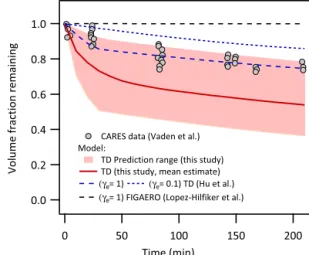
A test for these various parameter values is to use them to recreate data from other (non-heating-based) perturbations of gas-particle partitioning. Figure 5 shows evaporation kinetics of OA upon continuous stripping of vapors under isother-mal (25◦C) conditions simulated using volatility
parame-ter values from multiple independent approaches. The sim-ulation framework used here is described elsewhere (Saha and Grieshop, 2016). The shaded region in Fig. 5 shows the prediction range applying dual-TD-derived parameter values from this study within estimated uncertainty ranges (cam-paign average and unified fits offi,γe=0.1 to 1) with initial
COAvalues from 2 to 10 µg m−3anddp=100 and 150 nm.
Simulations are also shown with the OA volatility distri-bution from Hu et al. (2016) and FIGAERO-CIMS-derived OA volatility distribution (Lopez-Hilfiker et al., 2016) from Centreville measurements. The room temperature evapora-tion data from Vaden et al. (2011) measurements of ambi-ent aerosols during the Carbonaceous Aerosols and Radiative Effects Study (CARES-2010) field campaign in Sacramento, California, are also shown. This study attributed the observed slower-than-expected evaporation to extreme kinetic limita-tions to mass transfer (γe≪0.1). Although a direct
com-parison of observations collected in California and simula-tions based on volatility distribusimula-tions from Centreville is not ideal, the consistency of volatility behavior across our and other sites (Fig. 2, Table 1) suggests it is reasonable. Fig-ure 5 shows that these data fall within the range of values simulated using our TD-estimated volatility parameter val-ues (γe≥0.1). The Hu et al. (2016) volatility distribution
withγe=1 also recreates these data. In contrast, simulations
with the FIGAERO-CIMS-derived OA volatility distribution (Lopez-Hilfiker et al., 2016) from Centreville measurements (assuming γe=1) predict almost zero evaporation (dashed
black line in Fig. 5). This distribution thus appears to be
in-1.0
0.8
0.6
0.4
0.2
0.0
Volume fraction remaining
200 150
100 50
0
CARES data (Vaden et al.) Model:
TD Prediction range (this study) TD (this study, mean estimate)
(γe= 1) (γe= 0.1) TD (Hu et al.)
(γe= 1) FIGAERO (Lopez-Hilfiker et al.)
Time (min)
Figure 5.Isothermal evaporation kinetics of OA at 25◦C (room temperature) upon continuous stripping of vapors. Shaded region shows the evaporation kinetic model prediction range applying TD-derived volatility parameter values from this study; solid line shows the mean estimate. Dashed lines show model predictions using the OA volatility distribution derived using alternative approaches dur-ing the Centreville campaign (Hu et al., 2016; Lopez-Hilfiker et al., 2016). Symbols show experimental data from Vaden et al. (2011) collected during the CARES-2010 field campaign in California.
consistent with our observations and those from room tem-perature evaporation experiments.
3.4 Temporal variation of OA volatility
A time series of OA volatility distributions extracted over the campaign period is shown in Figs. 6 (Centreville) and S10 (Raleigh). The volatility distributions (fi)were extracted as described above from ∼6 h windows with fixed 1Hvap=
100 kJ mol−1andγe=0.5 based on the best estimates from
campaign-average fits. The average and 95 % confidence in-tervals ofC∗(µg m−3)are 0.18 (0.05–0.54) and 0.16 (0.04–
0.43) for the Centreville and Raleigh datasets, respectively, in line with values from the campaign-average and unified fits. The OA volatility distributions do not vary dramatically over the campaign period for either site.
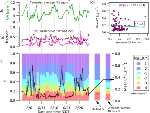
Ambient OA concentrations (COA)are shown in Fig. 6a (Centreville) and S10a (Raleigh). Figure 6b shows a time se-ries of the fractional contribution of isoprene-derived OA and more-oxidized oxygenated OA (MO-OOA) (Xu et al., 2015a, b) to total OA during the Centreville campaign. In a few low-COAinstances,C∗was found to be higher, but there was no
strong relation between these two quantities (see Fig. S12, scatter plot of meanC∗vsCOA). The relative contribution of
MO-OOA toCOAin many of these higher-C∗instances was
(a)
(d)
(b)
(c)
Figure 6.Time series of(a)ambient organic aerosol concentrations,COA;(b)fractional contribution of isoprene OA and more-oxidized oxygenated OA (MO-OOA) to total OA determined from PMF analysis; and(c)OA volatility distribution (fi)and meanC∗(open black
circles) during the Centreville campaign. All data are averaged over∼6 h (the time resolution offidistribution). Panel(d)shows a scatter
plot of meanC∗versus isoprene-OA fraction inCOA. Figure S10 shows similar analysis results for the Raleigh dataset.
OA contributed∼17–18 % to the campaign-averageCOAat
the Centreville site during the SOAS (Hu et al., 2015; Xu et al., 2015a, b), while MO-OOA contributed ∼39 % (Xu
et al., 2015a, b). Lopez-Hilfiker et al. (2016) reported that isoprene-derived OA was more volatile than the remaining OA using FIGAERO-CIMS measurements at the Centreville site. This result contradicts Hu et al. (2016), who reported a lower volatility of isoprene-derived OA than the bulk OA using TD measurements at the same site. Since our derived volatility distributions are for the bulk OA, we cannot make a specific comment on the volatility of isoprene-derived OA. However, if the volatility of isoprene-derived OA differs sub-stantially from the remaining bulk, OA volatility might be ex-pected to covary with the fractional contribution of isoprene-OA to COA. Figure 6c shows extracted bulk-OA volatility
distributions and their mean C∗ over the Centreville cam-paign period. Figure 6d shows a scatter plot of meanC∗vs.
the fractional contribution of isoprene-OA to COA; the two
show no correlation. Neither were statistically significant re-lationships found between the isoprene-OA fraction andfiin any particular C∗bin (see Table S2). These results indicate that the effective volatility of isoprene OA may not be sub-stantially different than the remaining bulk OA. If there is a difference, we are not able to detect it in our fits, potentially due to covarying contributions from other OA components.
Diurnal trends in OA volatility distributions are shown in Figs. 7 (Centreville) and S11 (Raleigh). Results show that
OA appeared less volatile in the afternoon than early in the morning for both sites (Centreville: campaign-average C∗ (µg m−3) in the morning∼0.25, afternoon ∼0.13 and
Raleigh: morning ∼0.2, afternoon ∼0.12). This trend is
consistent with previous field measurements in Mexico City (MILAGRO) and Riverside (SOAR-1) (Huffman et al., 2009). Figure 7a shows diurnal trends of OA factors derived from PMF analysis during the Centreville campaign (Xu et al., 2015a, b). Less-oxidized oxygenated OA (LO-OOA, av-erage O : C∼0.63) dominated in the early morning (∼40–
50 %), while more-oxidized oxygenated OA (MO-OOA, av-erage O : C∼1.02) was the largest OA component in the
af-ternoon (∼50 %). Xu et al. (2015a) hypothesized that
ox-idation of monoterpenes forms a large portion of observed LO-OOA in the southeastern US via NOxand O3(NO3
0.8 0.4
0.0 5 10 0.0150.40.8 20
0 (a)
(b)
(c)
f
Figure 7.Campaign-average diurnal trends for the Centreville mea-surements of(a)concentrations of total OA and OA factors,(b)OA volatility (fi and mean C∗), and (c) OA MFR after heating at
60, 90, and 120◦C with a TD residence time of 50 s. Figure S11 shows similar analysis results for the Raleigh dataset. PMF factors in panel(a)are LO-OOA: less-oxidized oxygenated OA; MO-OOA: more-oxidized oxygenated OA; and isoprene-OA: isoprene-derived OA (for details on OA factors analysis see Xu et al., 2015a, b).
contrast, bulk OA was dominated by MO-OOA in the after-noon. That OA is relatively less volatile in the afternoon is consistent with the observation that OA volatility often de-creases with increased oxidation (during functionalization) (Jimenez et al., 2009). Figure 8 shows scatter plots ofC∗vs.
LO-OOA and MO-OOA fractions of OA during the Centre-ville campaign. Although the average slopes of the scatter plots show an increase (decrease) ofC∗with increasing
LO-OOA (MO-LO-OOA) fraction these correlations are not strong (correlation coefficient, r∼0.5). Similar levels of
correla-tion were found with effective C∗ (Fig. S13). A poor cor-relation betweenC∗and OA factors is also observed in the
Raleigh dataset. For example, Fig. S14 shows scatter plots of C∗ vs. tracer (m/z)-based HOA fraction and OOA
frac-tion estimates (Ng et al., 2011b) with an average slope of
−0.3±0.16 (r∼0.2) for HOA and−0.12±0.11 (r∼0.1)
for OOA.
3.5 Average volatility and oxidation state of OA Figure 9 explores the link between average carbon oxida-tion state, OSc, calculated as 2×O : C – H : C (Kroll et al.,
2011), andC∗. O : C and H : C are estimated from an
em-pirical parameterization of the OA elemental ratio from unit mass resolution data, given by Canagaratna et al. (2015) as a function of f44 (O : C=0.079+4.31×f44) and f43
(H : C=1.12+6.74×f43−17.77×f432), respectively. f44
andf43are the fractional ion intensity atm/z44 and 43, re-spectively, taken from ACSM measurements. The estimated OA elemental ratios using the empirical parameterizations above are in relatively good agreement with those deter-mined via elemental analysis of the high-resolution mass spectra data (HRToF-AMS) collected by other groups during SOAS. For example, our estimated campaign-average O : C during the Centreville campaign (0.68±0.07) is within 1–2
standard deviations of that determined in Xu et al. (2015b) (∼0.78).
The scatter plot of OSc vs. C∗ (Fig. 9) shows a mild
downward trend, which suggests that lower-volatility OA is associated with higher oxidation state. However, the cor-relation is not statistically robust (r< 0.3). This is consis-tent with the observations of Xu et al. (2016) and Paciga et al. (2016) who reported weak association between average oxidation state and volatility for OA measured in the Lon-don and Paris areas, respectively. The campaign-average OSc
during the Centreville measurements (−0.18±0.15) was
higher than in Raleigh (−0.42±0.16) (p value≪0.0001),
whereas campaign-averageC∗values were essentially
iden-tical (Centreville: 0.18±0.14, Raleigh: 0.16±0.12 µg m−3;
pvalue > 0.1).
3.6 Application of measured volatility distribution to evaluate simulated OA in a CTM
Figure 10 compares the measured and simulated OA volatil-ity distributions at Centreville for June 2013. The simulated OA volatility distribution in theC∗ bins between 100 and 101µg m−3 agrees reasonably well with observations. The
model predicts a dominance of BSOA in the two bins, con-sistent with observations in the Centreville region. However, large discrepancies exist between the observed and simulated OA volatility distribution in theC∗ bins between 10−2 and 10−1µg m−3. The model tends to greatly underpredict the
OA concentrations in this volatility range. WRF/Chem did not reproduce the observed portion of the mass of OA in the lowerC∗ bins, from 10−4 to 10−1µg m−3, because the
low-0.6
0.4
0.2
0.0
Mean C* (µ
g m
-3 )
0.8 0.6 0.4 0.2 0.0
LO-OOA fraction r =0.5 (Slope = 0.45 ± 0.1)
r =0.48
(Slope = - 0.57 ± 0.12)
(a) (b)
Figure 8.Scatter plot of meanC∗versus(a)LO-OOA fraction, and(b)MO-OOA fraction in total OA concentration during the Centreville campaign.
-0.6 -0.4 -0.2 0.0 0.2
Mean OSc
(2 x O:C - H:C)
0.7 0.6 0.5 0.4 0.3 0.2 0.1 0.0
Mean C* (µg m-3) Centreville campaign average
Raleigh campaign average
r = 0.25
r = 0.20
Data : Centreville Raleigh Centreville (slope = - 0.29 ± 0.13) Raleigh (slope = - 0.23 ± 0.16)
Figure 9.Mean oxidation state(OSc)vs. mean volatility(C∗) mea-sured during the Centreville and Raleigh campaigns. Dots are cam-paign data, dashed lines are linear regression fits of data, and sym-bols are the campaign average with error bar showing±1 standard deviation.
volatility materials are missing in the WRF/Chem simula-tion.
The simulated total OA mass concentration (COA)was un-derpredicted by a factor of 2 to 3 at Centreville during the SOAS period. Several factors may contribute to this under-prediction. Comparison of WRF/Chem predictions of most relevant meteorological variables and major precursor VOCs with measurements collected during the SOAS shows a rela-tively good agreement. For example, the mean biases for sim-ulated temperature at 2 m, relative humidity at 2 m, and wind speed at 10 m are −0.9◦C,−0.8 %, and 0.3 m s−1,
respec-tively. The normalized mean bias (NMB) of the simulated planetary boundary layer height (PBLH) is −38 %, which
would tend to bias OA concentrations high, suggesting that the underprediction in PBLH is not responsible for the un-derpredictions of OA. In terms of VOC concentrations, the model performs well for β-pinene and formaldehyde with
Figure 10.Comparison between measured OA volatility distribu-tions and those simulated in WRF/Chem over the Centreville re-gion. Bar height is mean and error bar is±1 standard deviation of distributions extracted from measurements and simulations for June 2013. The inset shows a two-bin comparison (bin 1:C∗≤ 1 µg m−3and bin 2:
C∗=10 µg m−3). Simulated OA components include ASOA (anthropogenic-SOA), BSOA (biogenic-SOA), POA (primary-OA), and SVOA (semivolatile OA formed via oxidation of evaporated POA).
NMBs of −8.5 and −4.3 %, respectively, but it
underpre-dictsα-pinene with an NMB of−51.7 % and significantly
treatment in WRF/Chem include the coarse spatial resolution in the model simulation, the assumed fraction of OA added for each oxidation or aging step, the assumed fragmented and functionalized percentages of organic condensable va-pors, and the uncertainties in the dry- and wet-deposition ve-locities of SOA and SOA precursors. These factors can also contribute to the discrepancies between the model and ob-servedCOAat Centreville.
One likely contributor to the model’s underprediction is issues with the SOA yield parameterizations in the model. Smog chamber growth-experiment-derived mass yield coef-ficients (i.e., distributions of product mass yield in differ-ent volatility and/orC∗ bins) (Pathak et al., 2007) are used to model SOA in a CTM. The estimated SOA yield from a traditional smog chamber experiment could be underesti-mated due to wall losses of condensable vapors. For exam-ple, Zhang et al. (2014) showed up to a factor of 4 yield underestimation for toluene SOA due to this effect. The high- and low-NOx mass yields used in WRF/Chem simu-lations for ASOA and BSOA are based on traditional smog chamber yield experiments taken from Lane et al.(2008a). These distributions do not consider mass yields from the C∗ bins 10−4 to 10−1µg m−3, where a significant portion of the OA mass was observed. The substantial amounts of low-volatility materials are typically missing in these tradi-tional yield-measurement-based distributions (Kolesar et al., 2015b; Saha and Grieshop, 2016). Our recent dual-TD-based effort to determine the SOA mass yield distribution for α-pinene ozonolysis (Saha and Grieshop, 2016) indicates that products are substantially less volatile than the parameteriza-tions used in current models (including that discussed above). This α-pinene product distribution suggests a factor of 2– 4 greater SOA yield under atmospherically relevant condi-tions compared to traditional distribucondi-tions from smog cham-ber growth experiments. Updating SOA mass yield coeffi-cient data is likely required for all known precursors and may lead to large improvements in model predictions of bothCOA
and OA volatility distributions.
The WRF/Chem simulation used the semiempirical1Hvap
correlation derived by Epstein et al. (2010) (1Hvap=130−
11log10C∗, 298 K), which gives higher values, with a steeper log10C∗ dependence than our TD-derived values (∼80–
100 kJ mol−1). The difference in 1H
vap values used in
WRF/Chem and our TD-derived values should not have a significant effect on the comparison shown in Fig. 10. This is because the modeled–measured OA volatility compari-son was made at temperatures (SOAS campaign-average T =24.7◦C, WRF/Chem-simulated campaign-averageT =
23.8◦C) very close to the VBS reference temperature
(25◦C). Murphy et al. (2011) also reported a low
sensitiv-ity of1Hvapwhen predicting surface OA loading during the
FAME-08 study using a 2D-VBS framework. However, the effect of 1Hvap could be significant when simulating OA
loading at low ambient temperatures and high altitudes.
4 Conclusions and implications
This paper presents results from ambient-OA volatility mea-surements from two sites in the southeastern US under di-verse conditions. Measurement campaigns were conducted at a BVOC-dominated forested rural setting during summer and another more anthropogenically influenced, but forested urban location under cooler conditions. This study applied a dual-thermodenuder (dual-TD) setup that varied temperature and residence time in parallel. Ambient OA gas-particle par-titioning parameter (C∗, 1H
vap, γe)values were extracted by fitting observed dual-TD data using an evaporation ki-netic model. The OA volatility distribution derived via in-verse modeling is sensitive to1Hvapandγevalues. The
ad-dition of variable residence time TD (VRT-TD) data pro-vided tighter constraints on the extracted parameter values. A1Hvapof∼100 kJ mole−1andγeof 0.5 best explain
ob-servations collected at both sites under diverse conditions. An effective γe value of ∼0.1 to 1 can explain observed
evaporations within variability, while a very smallγe value
(γe≪0.1) cannot fit the observations from both TDs. The
Epstein et al. (2010) 1Hvap correlation, which was
deter-mined based on measured properties of a variety of known compounds, also did not reproduce the evaporation observed in this study.
While measurement campaigns were conducted under dif-ferent meteorological conditions at locations with varying levels of biogenic and anthropogenic emissions, the OA volatility distributions derived are found to be very similar. A substantial amount of OA (40–70 %) at both sites was found to be of very low volatility (C∗≤0.1 µg m−3)and will
re-main predominantly in the particle phase (effectively non-volatile) under typical atmospheric conditions. OA volatility distributions also did not vary substantially over the cam-paign period. Our derived OA volatility parameterizations appear to be broadly consistent with observations of room temperature evaporation (Vaden et al., 2011) during CARES-2010 in California. The observed consistency in OA volatil-ity across diverse settings is an important finding, which im-plies that OA in the atmosphere formed from a variety of sources can exhibit similar volatility properties and chemi-cal signatures. This result also suggests that measurements of OA volatility distributions such as derived here provide good diagnostics for overall model representativeness but may not be as useful for diagnosing differences across sites and con-ditions.
The diurnal profile of extracted OA volatility showed that bulk OA was less volatile in the afternoon than early in the morning. This trend is consistent with the prevalence of LO-OOA (less oxidized) in the morning and MO-LO-OOA (more oxidized) in the afternoon. However, while average O : C and/or oxidation state (OSc) of bulk OA is often considered
linked to volatility, in our datasets correlations between mean oxidation state(OSc) and mean volatility (C∗) were weak
at-mospheric OA is a complex mixture of organics with a broad range of volatilities and oxidation states reinforces the need to measure and understand the distribution of both volatility and oxidation states. The two-dimensional VBS framework (Donahue et al., 2012) offers one way to constrain these pa-rameters in atmospheric models. While determination of OA volatility distributions was the focus of this study, future ef-forts should also measure distributions of volatility and oxi-dation states comprising ambient OA.
The gas-particle partitioning parameters (C∗,1H vap,γe)
extracted from these measurements have important implica-tions for the treatment and evaluation of OA in current atmo-spheric models. Since a CTM incorporating the VBS frame-work predicts OA concentrations in each volatility (log10C∗) bin (i.e., OA volatility distribution), comparison of simulated and measured OA volatility distribution is a useful means for model evaluation beyond only comparing total OA concen-tration (COA). Here, we compared our measured OA
volatil-ity distribution with that simulated by WRF/Chem. This eval-uation indicates that OA volatility distributions predicted in WRF/Chem are inconsistent with measurements over theC∗ range from 10−4to 10−1µg m−3. This may give important
clues towards the root causes of the model’s underestima-tion of COA by a factor of 2 to 3. In comparison to our
TD-derived OA volatility distribution and other recent evi-dence (Ehn et al., 2014; Hu et al., 2016; Jokinen et al., 2015; Kokkola et al., 2014; Lopez-Hilfiker et al., 2016; Saha and Grieshop, 2016), low-volatility materials are mostly missing from the WRF/Chem predictions. Recent evidence of SOA from aqueous-phase oxidation in presence of abundant par-ticle water (Carlton and Turpin, 2013; Marais et al., 2016), formation of oligomers, and large molecular compounds di-rectly in the gas phase (Ehn et al., 2014) and via condensed-phase chemistry (Kroll et al., 2015; Kroll and Seinfeld, 2008) suggest that complex and multiphase formation and evolu-tion processes produce SOA in the atmosphere. Many of these processes can produce very-low-volatility organics and most are not included in current CTMs. These low-volatility organics appear to make significant contributions to the at-mospheric OA budget and cloud condensation nuclei forma-tion (Jokinen et al., 2015).
The 1Hvap andγe values extracted here for atmospheric
OA in the southeastern US also have important implica-tions for predicting OA concentraimplica-tions in a CTM. First, a 1Hvapvalue of 30–40 kJ mol−1(Farina et al., 2010; Lane et
al., 2008b; Pye and Seinfeld, 2010) is typically assumed for modeling OA in a CTM, which is substantially lower than that suggested by our TD observations (∼100 kJ mol−1). An
increase of assumed 1Hvap value can increase atmospheric
OA burden and lifetime for a particular input volatility dis-tribution (Farina et al., 2010), especially at low ambient tem-peratures and high altitudes. Finally, a value ofγe≥0.1
in-dicates a gas-particle repartitioning timescale (Saleh et al., 2013) on the order of minutes to an hour under atmospher-ically relevant conditions (Np∼1000–5000 cm−3).
There-fore, the equilibrium phase-partitioning assumption typically made in CTMs should be reasonable for a prediction timestep of∼1 h.
5 Data availability
Some of the data used in this study are publicly available at https://data.eol.ucar.edu/dataset/373.049 (Grieshop et al., 2017). Other data can be obtained from the authors upon re-quest ([email protected]).
The Supplement related to this article is available online at doi:10.5194/acp-17-501-2017-supplement.
Acknowledgements. We thank Satoshi Takahama and his research
group at EPFL for their help and support during the SOAS campaign, Paul Shepson’s group (Purdue University) for BVOC data, SEARCH Network for temperature, relative humidity, mixing height, CO, and NOx data from the Centreville site. Operation of
the SEARCH network and analysis of its data collection are spon-sored by the Southern Co. and Electric Power Research Institute.
Funding was provided by start-up support from North Carolina State University, Raleigh, US. Andrey Khlystov acknowledges funding by the US EPA (grant 83541101). Contents of this publication are solely the responsibility of the authors and do not necessarily represent the official views of the US EPA. Furthermore, the US EPA does not endorse the purchase of any commercial products or services mentioned in the publication. Khairunnisa Yahya and Yang Zhang acknowledge funding from the National Science Foundation EaSM program (AGS-1049200) for WRF/Chem simulations and high-performance computing support from Stampede, provided as an Extreme Science and Engineering Discovery Environment (XSEDE) digital service by the Texas Ad-vanced Computing Center (TACC) (http://www.tacc.utexas.edu), which is supported by National Science Foundation grant number ACI-1053575 and Yellowstone (ark:/85065/d7wd3xhc) provided by NCAR’s Computational and Information Systems Laboratory, sponsored by the National Science Foundation and Information Systems Laboratory. Lu Xu and Nga L. Ng acknowledge National Science Foundation grant 1242258 and US Environmental Protec-tion Agency STAR grant RD-83540301.
Edited by: B. Ervens
Reviewed by: two anonymous referees
References