Misconduct in the banking industry : stock market reaction to settlement announcements

(1)

Misconduct in the banking industry:

stock market reaction to settlement

announcements

Francisco Carvalho

Professor Geraldo Cerqueiro

Supervisor

Lisbon, 5

th

January 2018

Dissertation submitted in partial fulfilment of requirements for the

International MSc in Finance, at Universidade Católica Portuguesa

(2)

i

ABSTRACT

This study investigates the impact of settlement announcements between international banks and regulators on the short-term stock market performance of the banks. Recurring to event study methodology, this analysis is focused in settlements larger than USD 100 million. The dataset is comprised of penalties imposed on 25 financial institutions indentified as Global Systemically Important Banks (G-SIBs), totaling 141 events from 2010 to February 2017. Results for the full sample show significant positive abnormal returns for different periods surrounding the event. Significant positive abnormal returns on the day before the announcement for non-USA banks suggest leakage of information before the information is made public. Regarding USA banks the market response, although positive, seems to be slightly delayed. The positive abnormal returns indicate that investors are pleased that litigation cases are concluded and that the terms of deals are better than expected. Partial tax deduction of financial penalties also contributes to the positive reaction. Analysis of the determinants of abnormal returns supports these arguments and reveals that investors penalize less efficient banks. Lastly, settlements involving payments with compensatory nature and violation of sanctions are particularly well received by the market and lead to larger abnormal returns.

(3)

ii

ABSTRACT (portuguese version)

Este estudo investiga o impacto que a divulgação de settlements entre bancos internacionais e reguladores tem na performance a curto prazo das ações dos bancos em bolsa. Recorrendo à metodologia de event studies, esta análise foca-se em settlements superiores a USD 100 milhões. Os dados utilizados consistem em multas impostas a 25 instituições financeiras identificadas como Global Systemically Important Banks (G-SIBs), totalizando 141 eventos desde 2010 até fevereiro de 2017. Os resultados para a amostra total mostram retornos anormais positivos significantes para períodos diferentes em torno do evento. Retornos anormais positivos significantes no dia anterior à divulgação para bancos não americanos sugerem a existência de fuga de informação antes da mesma ser tornada pública. Em relação a bancos americanos, a reação do mercado, embora positiva, parece ocorrer com algum atraso. Os retornos anormais positivos indicam que os investidores ficam agradados com a conclusão de litígios e que os termos acordados são mais vantajosos do que o esperado. A dedução parcial das multas para fins de impostos também contribui para a reação positiva. A análise aos determinantes dos retornos anormais sustenta estes argumentos e revela que os investidores penalizam bancos menos eficientes. Por último, settlements que envolvam pagamentos de natureza compensatória e violação de sanções são particularmente bem recebidos pelo mercado e levam a retornos anormais maiores.

(4)

iii

Acknowledgments

First, I would like to thank to my supervisor, Geraldo Cerqueiro, for sharing his knowledge and clarifying all doubts that emerged throughout the elaboration of this dissertation.

Second, I would like to thank to all my friends from Católica-Lisbon (CLSBE) for all the fruitful discussions and great moments we shared during the past two years. I also want to thank to all my long-time friends for being there whenever I needed the most.

Finally, I must thank my parents and grandparents for their continuous support and motivation during this important period of my life, and for everything they ever taught me.

(5)

iv

1. Introduction

The main purpose of this study is to extend prior research on corporate misconduct in the financial sector, by examining stock market reaction after public disclosure of settlements (and correspondent financial penalties) between banks and regulators that result in the conclusion of unsolved litigation. Different phases during corporate ligation could trigger different short-term market reactions. Previous research has shown that allegations of corporate misconduct lead to significant declines in the equity value of firms, as investors anticipate potential losses arising from litigation and reputational costs. With ongoing litigation, uncertainty about the final outcome is always present. This uncertainty leads investors to fear additional litigation-related costs and new enforcement actions being brought up against the firm by regulators. In fact, the uncertainty only vanishes when the case ends, usually under the form of a settlement or judgment. At this stage, several factors might prompt a positive reaction from investors (e.g. final outcome is known and firms get off lightly).

Using event study methodology, I investigate whether the announcement of settlements with regulatory agencies (in some cases private entities) has a significant impact on the market value of Global Systemically Important Banks (G-SIBs). Assuming that markets are efficient in the sense that all publicly available information is reflected in stock prices, if settlement announcements convey unexpected information, investors should react and stock prices will be affected. If this is verified, settlement announcements are considered informative. Additionally, in order to understand in more detail and explain the results of the event study, I study the cross-sectional information content of settlement announcements by analyzing if certain bank-specific and settlement-specific variables influence investors’ reaction upon the announcement of resolution of litigation.

The remainder of the study is organized as follows: Section 2 highlights the concepts behind misconduct and reputational risk. In Section 3 research related to this study is discussed. In Section 4 the methodology used throughout the study is provided. In Section 5 I describe the data used in the study and elaborate on how the dataset was created. Additionally, due to lack of research on this subject an overview of financial penalty trends is provided for banks in the sample. In Section 6 the empirical results are presented and analyzed. Lastly, Section 7 concludes.

(7)

2

2. Misconduct and reputational risk

Misconduct risk in banking has been growing consistently after the 2007-2009 global financial crisis because of stricter rules on financial intermediation and increased scrutiny by customers and regulators (Resti, 2017). Despite its harmful impact on both the financial stability of the banking sector and the real economy, misconduct risk does not have a single, precise definition. According to the European Banking Authority (EBA), misconduct risk is defined as “the current or prospective risk of losses to an institution arising from an inappropriate supply of financial services, including cases of willful or negligent misconduct” (European Banking Authority, 2016, p. 89).

Misconduct in banks may damage confidence in the financial system, which has been weakened since the emergence of the aforementioned financial crisis. Regulators and supervisors must ensure that banks are stable and safe, making the execution of enforcement actions an important tool that allows them to sanction banks whenever they violate safe banking practices or the law is broken. Ex post penalties in the form of fines are the most common determent method of regulators. They rely on the discouraging effect of a pecuniary fine, in addition to a reputational cost (Carletti, 2017). This is an important feature of banking supervision, since due to opaqueness of bank business models (Morgan, 2002), regulators must have clearer information than market participants.

While financial penalties rightly serve as a correcting mechanism, in certain cases, they may entail systemic risks and have a counterproductive effect for financial stability (European Systemic Risk Board, 2015). In fact, the European Banking Authority introduced in 2014, for the first time, costs related to misconduct risk in its EU-wide stress tests. Still, Köster and Pelster (2017) point out that for some commentators these litigation costs are just another cost of doing business. According to a report elaborated by The Boston Consulting Group (BCG), banks across the world have paid around USD 321 billion since 2009, and while U.S. regulators have been more effective in imposing penalties and recovering fines, their counterparts in Europe and Asia are likely to step up pace (The Boston Consulting Group, 2017).

Misconduct risk and reputational risk go hand in hand as reputational costs are usually a consequence of misconduct. Reputational risk is the “risk arising from negative perception on the part of customers, counterparties, shareholders, investors, debt-holders, market analysts, other

(8)

3

relevant parties or regulators that can adversely affect a bank’s ability to maintain existing, or establish new, business relationships and continued access to sources of funding” (Bank for International Settlements, 2009, p. 19). In sum, reputational risk is any risk that can potentially damage the status of an organization in the eyes of third-parties. Reputational costs arise because of the weakened confidence of stakeholders, which can be manifested, for example, in lower sales by a firm that engages in consumer fraud or unfavorable changes in the terms of trade with suppliers when a firm cheats in its commercial transactions (Murphy et al., 2009).

3. Literature review

In an institutional context, a firm’s choice to engage in erratic behaviors (i.e. misconduct) is the same as any other business decision (Simpson, 2002). Yet, the potential losses stemming from its detection should be weighed against the potential economic gains in case of impunity. According to Murphy et al. (2009) potential losses include costs resulting from litigation and reputational costs.

There is a considerable vast literature dealing with cross-industry firms accused of misconduct acts and the correspondent impact on the stock price. Karpoff and Lott (1993) were some of the first conducting research in this topic, and they analyze the market impact that firms experience after the initial press announcement that they are facing criminal charges. In a sample consisting of 132 corporate frauds from 1978 to 1987, the authors find that alleged or actual fraud announcements of stakeholders or the government correspond to significant losses in the accused firm’s common stock market value, with average abnormal declines of 1.3% and 5.1% respectively. They also find that around 6.5% is explained by penalties and legal fees, with the remaining loss being explained by reputational damages. Other studies present similar results (Alexander, 1999; Bhagat et al., 1994; Murphy et al., 2009; Reichert et al., 1996 Skantz et al., 1990).

With respect to short-term returns, it is not surprising that the first public disclosure of a firm’s misconduct should have a negative effect on the stock price, as shareholders anticipate the monetary losses that might emerge, such as financial penalties and legal costs, and also the resultant reputational damage (Haslem, 2005). Nonetheless, different events during corporate litigation could cause different reactions. The settlement or judgment is a crucial event in

(9)

4

corporate litigation, since only at this point the precise information about the extent of wrongful activities is publicly disclosed. Although it is likely that information about the misconduct has surfaced before the date of the settlement or judgment, there is uncertainty about its trustworthiness and whether if such information is definitive or not.

Köster and Pelster (2017) argue that upon a settlement or judgment a positive effect on the stock price is expected for several reasons. The resolution of litigation concludes a dispute, eliminates the uncertainty about the final outcome and puts an end to the costs arising from the negative media coverage of the process. A positive market reaction might also indicate that investors realize that firms get off lightly, as financial penalties might be small, when weighted against the realized gains accrued from the misbehavior or the provisions set aside. Additionally, the resolution of unsolved litigation and the correspondent financial penalties might also promote a change towards more elaborate governance mechanisms and contribute to more responsible practices by the management (Agrawal et al., 1999). In particular, settlements should be seen as good news for shareholders of the accused firms and as the optimal solution in litigation cases, because they reduce the risk of larger financial penalties when resolution is achieved through a judgment (Haslem, 2005).

Some authors have studied the short-term market reaction after settlement announcements but there is disparity among the results. Contrary to what would be expected, Haslem (2005) detects negative abnormal returns after a settlement is announced, and argues that self-interest prompts managers to settle at higher values even when it could be more benefic for shareholders not reaching a settlement. Other studies find a negative or insignificant effect of the settlement on stock prices (Karpoff and Lott, 1993, 1999). Conversely, Bhagat et al. (1994) and Koku and Qureshi (2006) find short-term positive abnormal returns.

When focusing only in the financial industry, the number of research investigating the impact of misconduct-related issues on the market value of banks is somewhat limited and scarcer than expected. Studies by Cummins et al. (2006), De Fontnouvelle and Perry (2005), and Gillet et al. (2010) analyze the reputational loss that financial companies experience after unexpected operational losses. De Fontnouvelle and Perry (2005) examine reputational damage following operational loss announcements for a sample of 115 worldwide listed banks from 1974 to 2004. The authors show that the announcement date has a significant, negative impact on the stock

(10)

5

price of the banks and that the reputational effect, measured by the difference of market value loss and the operational loss (relative to the market value), is larger when the operational loss is due to internal fraud. Cummins et al. (2006) perform a similar analysis for 403 listed USA banks and 89 listed USA insurance companies between 1978 and 2003, considering operational loss announcements larger than USD 10 million. They find that both types of firms experience significant negative price reactions with market value drops exceeding the amount of the operational losses. However, banks experience smaller negative impacts and the reputational effect is larger for high growth firms (measured by high Tobin Qs). Gillet et al. (2010)investigate the market reaction after the announcement of operational losses larger than USD 10 million for 152 financial companies listed in Europe and USA between 1990 and 2004. For each operational loss, key dates are defined and analyzed: the first press announcement, the recognition by the targeted company, and the settlement date. The authors discover significant negative abnormal returns around the first press date, while around the settlement date (when it differs from the two other dates) significant positive abnormal returns are detected. They also find that internal frauds trigger larger abnormal returns, and that USA financial companies suffer larger reputational losses than their European counterparts. Finally, Köster and Pelster (2017) examine the impact of financial penalties on banks’ market value and profitability. Their sample is comprised of 68 financial institutions from 20 different countries and only settlements or judgments higher than USD 10 million are considered. The authors find significant positive abnormal returns in the period surrounding the announcement of the settlement or judgment, and also in the one-year buy-and-hold returns. The arguments used to explain such reaction are: 1) improvement of the managers’ behavior and cessation of erratic behaviors after the payment of a fine; 2) investors’ sense of relief due to the magnitude of the penalty (when weighted against the economic gain achieved through misconduct); 3) partial tax deductibility of some financial penalties, partly offsetting their negative impact in banks’ results1; 4) elimination of uncertainty associated with pending litigation and cessation of negative media coverage.

(11)

6

4. Methodology

4.1 Event study methodology synthesis

An event study measures the impact of a specific event on the value of a firm (Mackinlay, 1997). More specifically, using this method, one can determine whether there is an abnormal stock price effect associated with an unanticipated event – that is, if the returns were different from those that would be considered appropriate (or normal), given a certain model used to obtain theoretically adequate returns. Studies by Ball and Brown (1968) and Fama et al. (1969) introduced the standard methodology that continues to be used today. Since analyzing each event individually is not very informative, the key focus is to measure the sample securities’ mean and cumulative mean abnormal returns around the time of an event (Khotari and Warner, 2006).

While there is not a single defined structure for conducting event studies, there is a general flow of analysis. Mackinlay (1997) summarizesthe procedure in seven steps:

First, it is mandatory to define what constitutes the event of interest and the period over which the security prices of the firms involved will be analyzed. This period is known as the event window. The second step consists in determining the selection criteria for the inclusion of a given firm in the study. Third, it is required to define and calculate the normal and abnormal returns (ARs) for each individual event. Several models can be used to calculate the normal returns (e.g. Market Model, Fama-French three Factor Model). After selecting which model to generate normal returns, the estimation window needs to be defined. This is the period over which the parameters of the model are estimated. Typically, the estimation window precedes the event window, so that the event does not influence the normal performance model estimates. This is the fourth step. Then, abnormal and cumulative abnormal returns (CARs) can be calculated in the event window. The fifth step is defining the testing framework for ARs and CARs. Important considerations are defining the null hypothesis and determining the techniques for aggregating the ARs. Several tests (parametric and non-parametric) can be used to access the statistical significance of ARs. However, the quality of test statistics is related to the characteristics of the data. Deviations of these characteristics from those required by statistical theory will worsen the quality of the test statistics. So, researchers must understand the statistical assumptions inherent to different tests and their limitations when hypothesis testing.

(12)

7

Common issues highlighted and examined by the literature are summarized by Binder (1998): 1) cross-sectional correlation (in event time) of abnormal returns estimators (particularly severe when all firms belong to the same industry or when there is event clustering; 2) heterogeneity of the abnormal return estimators variance; 3) serial correlation of abnormal return estimators for individual firms; 4) abnormal return estimators have greater variance during the event-period (also known as event-induced variance). While researchers must be aware of these specific characteristics, often many of the problems can simply be ignored, because, in practice, they are quite minor (Binder, 1998).

The sixth step is the presentation of empirical results, and the last step is interpretation of the results and conclusions obtained.

4.2 Defining events

Events are only considered when they have a final character, that is, when there is a settlement announcement. When there is more than one settlement on the same date for the same bank, penalties are added, constructing what I call aggregate financial penalties. Each aggregate financial penalty corresponds to one event and the minimum amount for inclusion is USD 100 million. In total, there are 195 individual financial penalties and 149 aggregate financial penalties. However, the number of events reduces to 141 due to the existence of concurring events.

4.3 Constructing abnormal returns

First, individual daily continuously compounded stock returns are calculated from closing prices (adjusted for capital events) retrieved from Thomson Reuters Datastream database. Each daily return is calculated from the previous day with a non-missing price and trading volume to the current day, using the following formula:

(1)

where is the daily continuously compounded return for stock on day , is the adjusted closing price for stock on day t, and is the adjusted closing price for stock on day . ARs are the actual returns of securities over the event window minus the normal, or expected,

(13)

8

returns over the event window. The normal returns are defined as the expected returns if no event had taken place. For each sample security , the abnormal return at time relative to the event is:

₍₂₎

where is the abnormal return, is the actual return, and is the normal return (given by a particular model of expected returns).

To calculate the ARs for each event, as in previous studies, the market model is used. The market model is a statistical model that relates the return of a security to the return of the market portfolio, as expressed in the following equation:

(3)

where is the stock return of the th bank on day , is the return of a market index on day , is the zero mean error term, is a parameter that measures the sensitivity of to the market index, and is a parameter that represents the idiosyncratic risk component of bank stock. The abnormal return of bank stock on day is estimated as the residual , and is defined as:

₍₄₎

In addition to the market model, a two-index model is also used to generate the abnormal returns. In this model, besides the standard market factor, it is also included an industry factor. The MSCI World Banks Index is chosen to proxy for the banking industry. This index is composed of large and mid cap stocks across 23 developed markets countries2. All securities are classified in the Banks industry group according to the Global Industry Classification Standard (GICS). The model is expressed as follows:

(5)

where is the stock return of the th bank on day , is the return of a market index on day , is the return of the banking industry index on day , is the zero mean error term, is a

2_{Developed Markets countries include: Australia, Austria, Belgium, Canada, Denmark, Finland, France, Germany,}

Hong Kong, Ireland, Israel, Italy, Japan, Netherlands, New Zealand, Norway, Portugal, Singapore, Spain, Sweden, Switzerland, U.K, and USA.

(14)

9

parameter that measures the sensitivity of to the market index, is a parameter that measures the sensitivity of to the banking industry index, and is a parameter that represents the idiosyncratic risk component of bank stock. The abnormal return of bank stock on day is estimated as the residual , and is defined as:

(6)

Lastly, for robustness of results, the Carhart (1997) four-factor model is also used to generate abnormal returns. This model is an extension of the Fama-French (1993) three-factor model (Fama and French, 1993), and is defined as follows:

(7)

where is the stock excess return of the th bank on day , is the return of a market index on day , is the average return on three small market capitalization portfolios minus the average return on three large market capitalization portfolios, is the average return on two high book-to-market equity portfolios minus the average return on two low book-to-market equity portfolios, is the average return on two high prior return portfolios minus the average return on two low prior return portfolios, is the zero mean error term, is a parameter that measures the sensitivity of to the market index, is a parameter that measures the sensitivity of to the size factor, is a parameter that measures the sensitivity of to the value factor, is a parameter that measures the sensitivity of to the momentum factor, and is a parameter that represents the idiosyncratic risk component of bank stock. The abnormal return of bank stock on day is estimated as the residual , and is defined as:

(8)

The indexes and datasets used per country for each return generating model are shown in

Appendix 1. The parameters in equations (3), (5) and (7) are estimated via Ordinary Least

Squares (OLS) over a specific estimation window. While there is no consensus in the literature regarding the length that should be used, the use of daily rather than monthly return data has become more prevalent (Khotari and Warner, 2006). One year of daily observations is used, that

(15)

10

is, 250 trading days. To check if results are dependent on estimation window length, 200 and 150 trading days are also used (not reported). Considering the event day, parameters are estimated for the following estimation windows: (-251, -2); (-201, -2); (-151, -2). Abnormal returns are calculated for each day of the (-1, 1) window. The chosen event window is short on purpose, since it only includes the day preceding the event, the event day and the day after the event. Nonetheless, it allows one to analyze possible leakage of significant information before the announcement, and the reaction in the trading day after if the information becomes public when markets are closed. With longer event windows the probability of existent concurrent events is higher, and this would result in the removal of more events from the analysis.

4.4 Common definitions

The estimation window length is , with as the latest day of the estimation window, and as the earliest day of the estimation window relative to the event day. The event window length is , with as the latest day of the event window relative to the event day. The sample size is defined as (i.e. number of events), and refers to the number of non-missing returns in the estimation window of bank .

Assuming that ARs are independent and identically distributed the equal-weighted average abnormal return (AAR) on a single-day period for a sample of events is calculated as:

(9)

The cumulative average abnormal return (CAAR) for multiple-day periods ( ,) for a sample of events is calculated as:

(10)

The variance of ARs for each bank is estimated over the estimation window as:

(16)

11

where is the number of parameters to estimate (2 if market model, 3 if two-index model and 5 if four-factor model).

4.5 Test statistics

The literature on event study test statistics is very rich, as is the range of significance tests. Usually, significance tests can be grouped into two separate groups: parametric and non-parametric tests. Parametric tests rely on assumptions about the distribution of ARs, as opposed to non-parametric tests which do not. To be certain that the results do not depend on a singular test, five parametric tests and two non-parametric tests will be used.

4.5.1 Ordinary -test

The ordinary -test is the standard parametric test statistic proposed by Mackinlay (1997). This method assumes that residuals are independent across events. It does not take into consideration cross-sectional correlation of residuals and the possibility of event-induced variance.

For single-day periods the test is asymptotically distributed under the null hypothesis of no event effect, and is defined as:

(12)

where is the variance of AARs, estimated as:

(13)

and is the variance of ARs, estimated for each firm during the estimation window as in equation (11) .

For multiple-day periods the test is asymptotically distributed under the null hypothesis of no event effect, and is defined as:

(17)

12

where is the variance of CAARs, estimated as:

(15)

4.5.2 Crude dependence adjustment test

To account for cross-sectional correlation of abnormal returns, Brown and Warner (1980, 1985) suggest that firms should be grouped into a portfolio, and the time series (in event time) of average portfolio residuals over the estimation window is used to calculate the standard deviation of AARs. This parametric test uses a single variance estimate for the entire portfolio. As a result, it does not consider unequal return variances across securities.

(16)

where is the standard deviation of the AARs, estimated as:

(17)

and is estimated as:

(18)

13 4.5.3 Patell test

In this parametric test, also known as “standardized residual test”, suggested by Patell (1976), residuals are first estimated as in the ordinary -test. However, before being aggregated over time and across events, they are standardized. This standardization adjusts for the fact that event-period residuals are out-of-sample predictions, thus having greater standard deviation than estimation-window residuals (Patell, 1976). Standardized values of residuals are obtained by dividing the event-period abnormal returns by the standard deviation of the estimation window, adjusted to reflect the forecast error (Boehmer et al., 1991). While this method assumes that residuals are cross-sectionally uncorrelated and that event-induced variance is insignificant, it allows for heteroskedasticity in event window residuals and helps prevent securities with large volatility from over-influencing the results. The adjustment in this test is only calculated for the market model residuals. For the other two models residuals are standardized by the square root of their variance, calculated as in equation (11).

The adjustment to the variance of ARs of each firm is:

(20)

where is the average market return over the estimation window.

Each AR is standardized for each time period over the event window, thus obtaining standardized abnormal returns (SAR):

(21) Then, SARs are aggregated for each time period over the event window, and cumulative standardized abnormal returns (CSAR) are calculated:

(19)

14

(23)

where is estimated as:

(24)

For multiple-day periods the SARs are first aggregated over time for individual firms:

(25)

(26)

(27)

4.5.4 Standardized cross-sectional test

Proposed by Boehmer, Musumeci and Poulsen (1991), this is a widely used parametric test can be considered a hybrid between the Patell (1976) and ordinary cross-sectional tests. First, residuals are standardized as in equation (21), and then, instead of using the estimation window for the calculation of the standard deviation, observations from the event-period are used to estimate the standard deviation of event-period residuals. Overall, this method benefits from the properties of the other two methods used to create this one. It allows for event-induced variance and heterogeneity in variances of residuals. However, it does not account for cross-sectional

(20)

15

correlation between events. The adjustment in this test is only calculated for the market model residuals. For the other two models residuals are standardized by the square root of their variance, calculated as in equation (11).

(28)

(29)

(30)

where is the standardized cumulative abnormal return for firm , estimated as:

(31) and is the corrected standard deviation proposed by Mikkelson and Partch (1998), estimated as: (32)

(21)

16 (33) 4.5.5 Calendar-time test

As pointed out by prior studies (e.g. Bernard, 1987; Collins and Dent, 1984), cross-sectional dependence across residuals may induce bias in standard errors, particularly when the event occurs in the same day for all firms, or when all firms belong to the same industry. When clustering occurs, it can be accommodated by aggregating residuals into portfolios based on calendar-time (Mackinlay, 1997). In this study all firms belong to the same industry, and there are events with the same calendar date for different firms. To account for this, Jaffe’s (1974) calendar time -test is adopted. To conduct this test, clustered events are formed into portfolios according to event date, i.e., events that occurred on the same day are grouped into one equal-weighted portfolio, and firms with isolated event dates correspond to single-security portfolios. Residuals are calculated for each portfolio, and based on the AARs for each portfolio during the estimation window a time series estimate of the standard deviation is obtained for each portfolio. Finally, like in the Patell (1976) test, the event-period residuals are standardized by dividing them by the estimated standard deviation. This method takes into account correlation between residuals and non-equal variances.

(34)

where is the number of portfolios and is the average standardized abnormal return, estimated as: ₍₃₅₎

where is the abnormal return of portfolio at event time and is the standard deviation of portfolio , estimated as in equation (11) but for portfolio residuals.

(22)

17

(36)

4.5.6 Cowan generalized sign test

This non-parametric test introduced by Cowan (1992) takes into account the fraction of positive residuals in the estimation window and compares it with the fraction of positive residuals in a certain event window. The null hypothesis is that the fraction of positive returns is the same as in the estimation window.

For both single and multiple-day periods the test is asymptotically distributed under the null hypothesis of no event effect, and is defined as:

(37)

where is the fraction of positive ARs or CARs for a certain event-period or event window, and is estimated as:

(38)

where is 1 if the sign is positive and 0 otherwise.

4.5.7 Corrado rank test

The rank test procedure proposed by Corrado (1989) is a widely used non-parametric test that treats the estimation and event window as a single set of returns, and assigns a rank to each firm’s residuals. Rank one is attributed to the smallest residual. is the rank of the abnormal return in the sample of residuals of firm . The ranks of the residuals of different days are dependent by construction. However, the effect of ignoring the dependence should be inconsequential for short event windows (Campbell and Weasley, 1993).

(23)

18

(39)

where is the average rank on event day t across N stocks, and is estimated as:

(40)

For multiple-day periods, the test proposed by Campbell and Wesley (1993) is utilized. The test is asymptotically distributed under the null hypothesis of no event effect, and is defined as:

(41)

where is the average rank across firms and time in event window, and is estimated as:

(42)

4.6 Cross-sectional analysis of CARs

The estimated abnormal returns are frequently used as the dependent variable in a regression with firm-specific characteristics as explanatory variables. Such an exercise can provide theoretical insights and is particularly helpful when multiple sources exist for the origin of the abnormal returns, since it is an appropriate tool to investigate this association (Mackinlay, 1997). To investigate the results of the event study in greater detail, CARs are regressed against a set of explanatory variables, as expressed in the equations below:

(24)

19

(44)

The (-1, 1) CAR of event is the dependent variable in a cross-sectional regression with the following firm-related explanatory variables: proxies for the size of the settlement , measured by the settlement amount divided by total assets of the correspondent bank at fiscal year-end prior to the settlement. is the pre-tax return on assets of the bank correspondent to event , measured by before-tax profitability divided by total assets, at fiscal year-end prior to the settlement. is the capitalization, measured by the ratio of common equity to total assets, at fiscal year-end prior to the settlement. is the size of the bank, measured by the natural logarithm of total assets, at fiscal year-end prior to the settlement. is the liquidity of the bank, calculated as the ratio of total loans to total deposits, at fiscal year-end prior to the settlement. proxies for the credit quality of the ban, measured as the ratio of allowance for loan losses to total assets, at fiscal year-end prior to the settlement. proxies for the portfolio risk of the ban, measured as the ratio of risk-weighted assets to total assets, at fiscal year-end prior to the settlement. is a measure of the solvency of the bank, measured as the Tier 1 capital ratio at fiscal year-end prior to the settlement. proxies for the efficiency of the bank, measured as the ratio of operating expenses to operating income, at fiscal year-end prior to the settlement. is the tax amount paid by the bank, calculated as taxes divided by pre-tax income, at fiscal year-end prior to the settlement. To investigate if settlement-specific characteristics affect CARs, the type of misconduct and the agency with whom the settlement was reached, measured by the dummy variables and are introduced into the regression analysis. Time dummies that control for the year in which settlement occurred are always included . All variable definitions and data sources can be consulted in Appendix

2. The selection of bank-specific characteristics aims to cover most of the structure of a bank and

is in line with several studies investigating the determinants of profitability of banks (e.g., Athanasoglou et al., 2008; Berger, 1995; Demirgüç-Kunt and Huizinga, 1999) and event studies focused in the banking industry (e.g., Asimakopoulos and Athanasoglou, 2013; Köster and Pelster, 2017; Murphy et al., 2009).

(25)

20

As pointed out by Gonedes and Dopuch (1974), the error terms in this regression might be heteroskedastic if the abnormal return estimators have these properties. Karafiath (1994, 2009) provides simulation evidence on statistical tests in cross-sectional regressions using diverse estimation methods and finds that more sophisticated alternatives do not show clear advantages over OLS and WLS approaches. Moreover, under certain conditions and with a large sample size, tests using OLS are unbiased and as powerful as the WLS approach. Therefore, as suggested by Mackinlay (1997), the cross-sectional regressions are estimated via OLS with heteroskedasticity-consistent standard errors, following White (1980), and also via WLS, with the weights for each observation corresponding to the inverse of the variance of the estimation period residuals.

5. Sample selection, data sources and financial penalty trends

5.1 Sample selection and data sources

Expenses related to misconduct are usually not presented in a clear and transparent way in the publicly available bank reports. Such expenses tend to be aggregated with other expenses, making it infeasible to obtain segregated values. Therefore, due to this serious constraint I follow a different approach. Using several reliable sources of financial information (e.g. Bloomberg, Financial Times and Reuters News), public information from regulators and supervisors (e.g. Financial Conduct Authority, Federal Housing Finance Agency), as well as Violation Tracker3

search engine, I collect data and build a hand-made dataset. This dataset includes the names of banks, the type of misconduct that originated the financial penalty, the amount of the penalty, the settlement date, and the entities imposing the penalty. Events are only considered when there is a settlement agreement. When there is more than one event on the same date for the same bank, the penalties are aggregated. To be included in the analysis, aggregate financial penalties have to be at least USD 100 million. Since not all settlements are reported in the press, it was decided that the sample would be composed of listed, well-known large banks that enjoy extensive media coverage. Considering this, all banks that used to be, and are currently included in the list of Global Systemically Important Banks (G-SIBs), published yearly by the Financial Stability Board (FSB), are included in the sample, as long as there is at least one event for the bank. The dataset

3_{Violation Tracker is a search engine on corporate misconduct that covers litigation cases initiated by 43 USA}

federal regulatory agencies and the Justice Department since 2010. For more information see: http://www.goodjobsfirst.org/violation-tracker

(26)

21

contains 25 banks from 9 different countries and a total of 195 individual financial penalties, that amount to 149 aggregate financial penalties for the period between 2010 and February 2017. However, due to the existence of concurring events that might trigger different reactions from the market the sample is reduced to 141 events. The list of banks included in the sample can be seen in Appendix 3, and the number of events per bank in Appendix 4. The number of events per regulatory entity is shown in Appendix 5.

Stock market data of banks and local market indexes is retrieved from Thomson Reuters Datastream database, while data used in the four-factor model is obtained from Kenneth French’s data library. All data obtained is daily. Accounting data is collected from Thomson Worldscope database and also from the annual reports made available by the banks. Since currency risk might lead to biased results (Irresberger et al., 2015), all accounting data is collected in US dollars.

5.2 Summary statistics and financial penalty trends

Since there is lack of empirical studies analyzing financial penalties in the banking sector, in this section I provide an overview of the data collected for the sample, with the goal of creating new knowledge about the magnitude and dynamics of such penalties. Information is reported for all banks in the sample, and separately for non-USA and USA banks.

Summary statistics of individual financial penalties for all banks in the sample are shown in the first row of Panel A in Table 1. There are a total of 197 individual penalties. The average penalty is USD 1.08 billion and the median is USD 0.34 billion. As the mean and median suggest, the distribution of individual financial penalties is considerably skewed to the right. In fact, 75% of all penalties range from USD 0.09 billion to USD 0.72 billion and 90% of all penalties fall between USD 0.09 billion and USD 2.10 billion. The largest individual financial penalty in the dataset is USD 16.65 billion. Of all the individual penalties, 95 correspond to non-USA banks and the remaining 102 to USA banks. The average penalty is higher for USA banks than for non-USA banks (USD 1.51 billion versus USD 0.60 billion), and the same is verified for medians (USD 0.37 billion versus USD 0.30 billion). For non-USA banks 75% of the penalties range between USD 0.09 billion and USD 0.52 billion, while for USA banks the penalties vary from USD 0.10 billion to USD 1.15 billion. For non-USA banks, the 10% largest penalties are above USD 0.95 billion, but for USA banks the 10% top penalties surpass USD 4.90 billion. The maximum penalty for non-USA banks is USD 8.97 billion versus USD 16.65 billion for USA

(27)

22 Table 1

Summary statistics

Statistic Obs Mean Median 75th P 90th P SD Min Max Kurt Skew

Panel A: Individual financial penalties

All banks 195 1.078 0.342 0.720 2.096 2.312 0.086 16.650 18.388 4.077

Non-USA banks 93 0.605 0.298 0.523 0.954 1.277 0.086 8.974 28.687 5.208

USA banks 102 1.509 0.374 1.150 4.900 2.896 0.100 16.650 11.114 3.250

Panel B: Aggregate financial penalties

All banks 149 1.410 0.410 1.080 3.330 2.676 0.100 16.650 12.865 3.449

Non-USA banks 63 0.893 0.340 0.822 2.324 1.571 0.100 8.974 15.097 3.730

USA banks 86 1.789 0.463 1.525 5.300 3.214 0.100 16.650 8.549 2.914

Panel C: Cross-sectional analysis variables

PEN 141 0.009 0.003 0.008 0.035 0.015 0.000 0.079 6.803 2.640 BTROA 141 0.006 0.005 0.011 0.013 0.006 -0.008 0.024 -0.189 0.304 CAP 141 0.079 0.087 0.104 0.112 0.027 0.025 0.129 -1.261 -0.268 SIZE 141 21.226 21.380 21.541 21.636 0.470 18.852 21.749 4.477 -1.807 LIQ 141 0.779 0.805 0.914 1.060 0.261 0.119 1.669 1.364 -0.163 CREDITQ 141 0.009 0.007 0.013 0.017 0.007 0.000 0.049 6.627 1.704 PORTFR 141 0.474 0.511 0.627 0.693 0.175 0.122 0.817 -1.086 -0.161 SOLV 141 0.132 0.129 0.137 0.163 0.019 0.093 0.213 2.094 1.211 EFF 141 0.747 0.743 0.862 0.959 0.148 0.447 1.156 -0.407 0.502 TAX 141 0.332 0.264 0.312 0.541 1.098 -0.692 7.287 33.256 5.560

This table presents descriptive statistics on individual financial penalties, aggregate financial penalties and for all variables used in the cross-sectional regression analysis. I report

the number of observations, mean values, median values, 75th_{and 90}th_{percentiles, standard deviation values, minimum values, maximum values, and also kurtosis and skewness}

(28)

23

banks. Summary statistics for aggregate financial penalties are shown in Panel B of Table 1. Of course, due to the aggregation process almost all statistics exhibit higher values but the same conclusions as before apply to aggregate financial penalties.

Fig. 1 to Fig. 3 show the number and total amount of individual financial penalties per year, for

all banks, non-USA banks and USA banks. The number and total sum of penalties strongly increased from 2011 to 2012, from 11 to 25, and total sums of USD 10.09 billion to USD 33.94 billion. The average penalty also increased from USD 1.19 billion to USD 1.36 billion. Non-USA banks were imposed more penalties than USA banks, but the latter were responsible for a total sum of USD 28.46 billion in settlements, as 2012 was the year in which USA authorities most notably started to go after banks and punish them for their role in the latest global financial crisis. In 2013 penalties grew once again both in number and value, with USA banks being responsible for more than USD 44 billion. However, 2014 stands as the year with the largest number of financial penalties and settlement amounts. Non-USA banks reached 26 settlements totaling almost USD 17 billion, while USA banks attained 21 settlements amounting to USD 45.5 billion. In 2015, despite being the year with the second largest number of penalties, it was the year with the lowest average settlement (USD 0.37 billion) since 2010. It was also the first year, in which non-USA banks’ settlements surpassed their American counterparts, totaling USD 9.73 and USD 5.22 billion respectively. In 2016 there was a considerable decrease in the number of settlements (40 to 23), but the total amount of penalties increased almost 3 billion. Finally, until the end of February of 2017 there was a total of 5 settlements, with two of them being particularly large, both corresponding to non-USA banks.

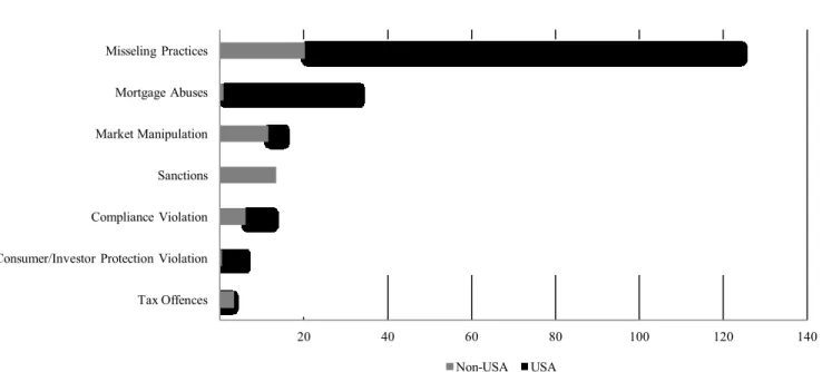
Fig. 4shows the total financial penalties paid by banks categorized into seven different groups. It is clear that non-USA banks and USA banks have essentially been punished for different kinds of misconduct. Financial penalties imposed to American banks arise mostly from two kinds of misconduct: misseling of financial products to investors and errors in foreclosure processes. Usually, such settlements are civil law cases, and the payments that the banks are obliged to make are compensatory in nature, therefore being tax deductible under USA tax law. On the contrary, non-USA banks have been penalized for, in addition to misseling towards investors, violation of sanctions and market manipulation. Therefore, a large part of settlements for non-USA banks corresponds to cases with criminal charges.

(29)

24 Fig. 1 – Number and total amount of financial penalties by year (2017 only includes 2 months): All Banks

Fig. 2 – Number and total amount of financial penalties by year (2017 only includes 2 months): Non-USA Banks

Fig. 3 – Number and total amount of financial penalties by year (2017 only includes 2 months): USA Banks

10 20 30 40 50 10 20 30 40 50 60 70 2010 2011 2012 2013 2014 2015 2016 2017 N um be r o f P en al ti es To tal A m ou nt (U SD b n)

Total Amount Number of Penalties

10 20 30 3 6 9 12 15 18 2010 2011 2012 2013 2014 2015 2016 2017 N um be r o f P en al ti es To tal A m ou nt U SD b n)

Total Amount Number of Penalties

10 20 30 10 20 30 40 50 2010 2011 2012 2013 2014 2015 2016 2017 N um be r o f P en al ti es To tal A m ou nt (U SD b n)

(30)

25 Fig. 4 - Total amount (USD bn) of financial penalties categorized into seven different groups. “Misseling Practices” mainly includes settlements involving the misseling of

mortgage-backed securities and credit default obligations. The grand majority of such settlements correspond to practices engaged during the period before and after the 2007-2009 global financial crises. “Mortgage Abuses” consists in settlements related to errors in foreclosure processes. “Market Manipulation” involves financial penalties applied to banks that engage in practices that are seen as manipulations of financial markets (e.g. LIBOR rigging). “Sanctions” includes penalties imposed to banks that engage in activities with countries present in USA’s OFAC sanctions list. “Compliance Violation” includes different violations against rules (e.g. anti-money laundering deficiencies). “Consumer/Investor Protection Violation” comprises different practices of misconduct that harm costumers or investors (e.g. discriminatory lending practices against minorities or misuse of customer cash). “Tax Offences” includes financial penalties imposed to banks that help customers to evade taxes.

20 40 60 80 100 120 140

Tax Offences Consumer/Investor Protection Violation Compliance Violation Sanctions Market Manipulation Mortgage Abuses Misseling Practices Non-USA USA

(31)

26

Misseling of financial products to investors (e.g. mortgage-backed securities or credit default obligations) is the source of more than half of the total financial penalties in the sample, with a total value of almost USD 125 billion. Banks from USA paid the majority of this amount, with a total of USD 104.40 billion. The main reason for this is that USA authorities started to charge banks earlier for their role in the most recent global crisis. Shortly after the crisis, President Barack Obama created several agencies and mechanisms to combat financial crime. Most notably, in 2012 the Residential Mortgage-Backed Securities (RMBS) Working Group was created. Its main goal is to “investigate and prosecute misconduct by financial institutions in the origination and securitization of mortgages”. There are 60 individual financial penalties of this kind in the sample. The average penalty in this category is around USD 2.1 billion, and the largest penalty is USD 16.65 billion, paid by Bank of America in 2014. In second place are financial penalties imposed to banks due to abuses in foreclosure processes, with a total amount of USD 33.64 billion. Again, banks from USA are responsible for almost the total amount. This is explained by the joint state-federal settlements with the biggest USA banks shortly after the crisis period, most notably the National Mortgage Settlement in 2012 and the Foreclosure Settlement Review in 2013. Although there are only 13 penalties of this type, the average penalty is the largest amongst all categories, with a value of USD 2.59 billion. The highest amount is USD 11.8 billion, correspondent to a settlement reached with Bank of America in 2012.

Penalties resulting from market manipulation rank third with a total value of USD 15.64 billion. Opposed to the two previous classes of misconduct, non-USA banks are responsible for the majority of the sum. The LIBOR (first disclosed in 2012) and Forex (first disclosed in 2013) scandals and their resulting settlements contribute heavily to this category. In both cases several big banks, acting as cartels, cooperated and engaged in erratic behaviors in order to achieve financial gains through the manipulation of benchmark interest rates and interest rate derivatives. There are 47 settlements in this category, with an average penalty of USD 0.33 billion. The largest penalty is USD 0.98 billion, paid by Deutsche Bank to the European Commission in 2013. Penalties imposed due to engaging in transactions with countries subject to USA sanctions amount to USD 13.40 billion, with an enormous (and the largest of this type) penalty of USD 8.97 billion imposed to BNP Paribas in 2014

(32)

27

representing more than half of this sum. On average, settlements in this category are around USD 0.91 billion. It is noteworthy to highlight that, in this sample, no USA banks have been penalized for this reason. Compliance violations seem to be common both in USA and non-USA banks, with a total amount of USD 12.88 billion for 36 different individual settlements, and an average penalty of USD 0.36 billion. Misconduct practices that may harm consumers and/or investors are more common in USA banks, with a total sum of roughly USD 6.50 billion for 19 individual penalties, and an average penalty of USD 0.34 billion. Lastly, penalties imposed due to helping clients to evade taxes are only verified in non-USA banks. In total, this is the most uncommon type of misconduct, with only 6 settlements, totaling USD 3.39 billion.

In terms of agencies with whom settlements are reached, the U.S Department of Justice (DOJ) is responsible for a total amount of USD 74.11 billion, most of which resulting from cases related to misseling of financial securities. The years with the largest sums were 2014 (USD 28 billion) and 2013 (USD 13 billion) In second comes the Federal Housing Finance Agency (FHFA) with a total sum of USD 35.94 billion, with almost the entirety of this amount corresponding to 2014 (USD 15.65 billion) and 2013 (USD 17.50 billion). Appendixes 6 to 10 report a detailed coverage of settlements per category, for all banks, non-USA banks and USA banks. Appendix 9 reports settlements per agency. Appendix 10 reports settlements per agency and category. The coverage includes the number of penalties, total sum, average, maximum and penalties.

6. Results

6.1 Event study results

As mentioned, there are a total of 141 events (see Appendix 11), of which 61 correspond to non-USA banks and the remaining 80 to USA banks. Fig. 5 shows the development of average returns from 4 trading days before the event to 4 trading days after the event for the full sample and for the MSCI World Banks Index. Even without the event study results, it seems clear that the settlement announcements have a positive impact on the price of stocks. The graph shows that the average sample returns on the 3 days surrounding the event are clearly higher than the MSCI World Banks Index average returns.

(33)

28 Fig. 5 – Evolution of average returns from 4 trading days before to 4 trading days after the settlement for the full sample and for the MSCI World Banks Index. Days are relative to

the event date (t=0).

-0.15% -0.05% 0.05% 0.15% 0.25% 0.35% -4 -3 -2 -1 0 1 2 3 4 A ve rage R et ur n Days Sample Banks

(34)

29

Event study results are shown in Table 2 for all banks, Table 3 for non-USA banks, and

Table 4 for USA banks.

Panel A of Table 2 reports the CAARs and test statistics for four different event windows based on the market model for all settlements. Panel B reports the same results based on the ARs generated through the two-index model. In Panel C the same results are presented based on the four-factor model. All models show that the market reaction is positive on the day of the event. The AAR is around 0.26% based on the market model, 0.22% based on the two-index model, and 0.30% assuming the four-factor model. Parametric tests show statistical significance in all models, but the generalized sign test is not significant in any of the models and the rank test only shows positive significance when the market and four-factor models are used. The CAAR on the three-day window (that includes the day before, the event day, and the day after the event) is the largest in absolute value of all windows analyzed for all models, with values of 0.72%, 0.66% and 0.64% corresponding to the market model, two-index model and four-factor model, respectively. All CAARs for the (-1, 1) window are significantly positive based on all tests, with the exception of the generalized sign test. The mean CARs are also positive and significant in two different two-day windows (both include the event two-day and one includes the two-day before and the other the day after the event). The CAAR for the (0, 1) window is the second largest in absolute value for all models (ranges from 0.49% to 0.56%), and also significant based on the parametric tests for all models and non-parametric tests for some models. Despite being the smallest in absolute value (varies from 0.39% to 0.43%) the mean CAR for the (-1, 0) window is also significantly positive based on most of the tests. To take into account the correlation between banks’ ARs when the event day is the same the calendar-time approach is also used for robustness. The results are shown in Appendix 12 and corroborate the results of the other parametric test statistics discussed above. By comparing the parametric and non-parametric approaches, it seems that the presence of extreme positive values might be over-influencing the results of the parametric tests, since non-parametric tests, particularly the generalized sign test, do not indicate positive abnormal performance in some windows. This is not surprising since each settlement is unique, in the sense that the outcome and terms reached depend on the specificities of each particular case. Additionally, media coverage of litigation cases is not homogeneous, and

(35)

30 Table 2

Cumulative abnormal returns following the resolution of litigation for all banks.

Panel A: Market Model

Observations 141 141 141 141 Window (0) (-1,1) (-1,0) (0,1) CAAR 0.0026 0.0072 0.0043 0.0056 Ordinary -test 2.191** 3.459*** 2.530** 3.256*** CDA test 2.135** 3.371*** 2.465** 3.173*** Patell test 2.427** _3.451*** _2.587*** _3.357*** BMP test 2.297** 3.543*** 2.566** 3.452***

Generalized sign test 1.547 1.547 1.378 1.378

Corrado rank test 1.701* 2.479** 1.922* 2.317**

Panel B: Two-Index Model

Observations 141 141 141 141 Window (0) (-1,1) (-1,0) (0,1) CAAR 0.0022 0.0066 0.0039 0.0049 Ordinary -test 1.970** 3.407*** 2.489** 3.077*** CDA test 1.880* 3.252*** 2.376** 2.937*** Patell test 2.086** 3.188*** 2.375** 3.004*** BMP test 1.913* 3.251*** 2.326** 3.060***

Corrado rank test 1.254 1.980** 1.539 1.773*

Panel C: Four-Factor Model

Observations 141 141 141 141 Window (0) (-1,1) (-1,0) (0,1) CAAR 0.0030 0.0064 0.0039 0.0055 Ordinary -test 2.856*** 3.546*** 2.649*** 3.713*** CDA test 2.829*** 3.513*** 2.624*** 3.679*** Patell test 3.203*** 3.679*** 2.808*** 3.963*** BMP test 3.065*** 3.849*** 2.897*** 4.112***

Generalized sign test 1.114 2.630*** 1.283 2.293**

Corrado rank test 2.197** 2.631*** 1.787* 2.989***

This table presents the CAARs and correspondent significance tests for all banks in the sample for different event windows. Panel A reports the results based on the market model abnormal returns, Panel B shows the results based on the two-index model abnormal returns, and Panel C presents the results based on the four-factor model abnormal returns. Parameters for all models are estimated over a 250-day estimation window. Statistical significance of CAARs was

assessed using the parametric and non-parametric tests described in section 4.5.BMP Test is referred to as standardized

cross-sectional test within the text. Statistical significance is indicated by ***_,**_{, and}*_{at the 1%, 5% and 10% levels,}

(36)

31 Table 3

Cumulative abnormal returns following the resolution of litigation for non-USA banks.

Observations 61 61 61 61 Window (0) (-1,1) (-1,0) (0,1) CAAR 0.0028 0.0075 0.0051 0.0052 Ordinary -test 1.465 2.293** 1.903* 1.942* CDA test 1.490 2.332** 1.935* 1.974* Patell test 1.937* _2.508** _2.491** _1.951* BMP test 2.433** 2.760*** 2.817*** 2.276**

Generalized sign test 1.914* 0.890 1.146 1.146

Corrado rank test 2.112** 1.969** 2.347** 1.558

Observations 61 61 61 61 Window (0) (-1,1) (-1,0) (0,1) CAAR 0.0022 0.0066 0.0046 0.0041 Ordinary -test 1.265 2.160** 1.873* 1.667* CDA test 1.300 2.220** 1.925* 1.713* Patell test 1.791* 2.456** 2.467** 1.807* BMP test 1.952* 2.747*** 2.696*** 2.090**

Generalized sign test 2.216** 1.447 0.935 1.447

Corrado rank test 1.929* 1.929* 2.433** 1.294

Observations 61 61 61 61 Window (0) (-1,1) (-1,0) (0,1) CAAR 0.0027 0.0078 0.0046 0.0059 Ordinary -test 1.473 2.488** 1.782* 2.306** CDA test 1.483 2.505** 1.795* 2.322** Patell test 1.743* 2.758*** 2.184** 2.426** BMP test 1.970** 2.909*** 2.427** 2.596***

Generalized sign test 0.380 2.173** 0.892 1.404

Corrado rank test 1.466 2.128** 1.623 2.019**

This table presents the CAARs and correspondent significance tests for non-USA banks for different event windows. Panel A reports the results based on the market model abnormal returns, Panel B shows the results based on the two-index model abnormal returns, and Panel C presents the results based on the four-factor model abnormal returns. Parameters for all models are estimated over a 250-day estimation window. Statistical significance of CAARs was assessed using the

parametric and non-parametric tests described in section 4.5.BMP Test is referred to as standardized cross-sectional test

(37)

32 Table 4

Cumulative abnormal returns following the resolution of litigation for USA banks.

Observations 80 80 80 80 Window (0) (-1,1) (-1,0) (0,1) CAAR 0.0026 0.0070 0.0037 0.0058 Ordinary -test 1.629 2.590*** 1.687* 2.638*** CDA test 1.436 2.283** 1.487 2.325** Patell test 1.531 2.392** _1.259 _2.753*** BMP test 1.252 2.331** 1.153 2.605***

Corrado rank test 0.507 1.567 0.602 1.676*

Observations 80 80 80 80 Window (0) (-1,1) (-1,0) (0,1) CAAR 0.0022 0.0067 0.0034 0.0054 Ordinary -test 1.513 2.642*** 1.659* 2.647*** CDA test 1.319 2.303** 1.446 2.307** Patell test 1.205 2.088** 0.999 2.410** BMP test 0.996 1.996** 0.915 2.258**

Generalized sign test -0.196 0.699 0.475 0.251

Corrado rank test 0.121 1.011 0.099 1.225

Observations 80 80 80 80 Window (0) (-1,1) (-1,0) (0,1) CAAR 0.0032 0.0053 0.0034 0.0052 Ordinary -test 2.652*** 2.541** 1.985** 3.003*** CDA test 2.493** 2.389** 1.866* 2.823*** Patell test 2.730*** 2.476** 1.820* 3.143*** BMP test 2.361** 2.562** 1.779* 3.171***

Generalized sign test 1.148 1.595 0.924 1.818*

Corrado rank test 1.643 1.674* 0.997 2.215**

This table presents the CAARs and correspondent significance tests for USA banks for different event windows. Panel A reports the results based on the market model abnormal returns, Panel B shows the results based on the two-index model abnormal returns, and Panel C presents the results based on the four-factor model abnormal returns. Parameters for all models are estimated over a 250-day estimation window. Statistical significance of CAARs was assessed using the

parametric and non-parametric tests described in section 4.5.BMP Test is referred to as standardized cross-sectional test

Misconduct in the banking industry : stock market reaction to settlement announcements