Development of a photovoltaic system for horticultural greenhouses

Development of a photovoltaic system

for horticultural greenhouses

Nelson Jonas Gaspar

Master dissertation in Mechanical Engineering

Supervisor

Professor Armando Oliveira

Mestrado Integrado em Engenharia Mecânica

Abstract

The elaboration of this dissertation arose due from the possibility of reducing operational costs in greenhouses, using a photovoltaic system to provide electrical energy to all the consuming equipment. These include both stationary (lighting, pumping) and movable devices (transportation carts).

The objectives of this project are focused on the study and design of different solutions of photovoltaic systems in order to obtain the best cost/production ratio. A variety of solutions solutions varying in peak power, connection to the electrical grid and use of battery storage were analysed.

An evaluation of the implementation of these systems in horticultural greenhouses in the north of Portugal, more precisely in Póvoa de Varzim, was carried out.

Resumo

A elaboração da presente dissertação surgiu devido à possiblidade de redução de custos operativos em estufas agrículas, recorrendo à utilização de um sistema fotovoltaico de modo a fornecer energia elétrica a todos os equipamentos consumidores eletricidade. Estes incluem dispositivos fixos (iluminação, bombagem) e móveis (carros transportadores).

O projeto centrou-se no dimensionamento e estudo de várias soluções de sistemas fotovoltaicos, de forma a obter a melhor relação custo/produção. Para tal foram analisadas várias soluções de sistemas variando na potência de pico, ligação à rede elétrica e existência de baterias para armazenamento da electricidade produzida em excesso. Foi feita uma avaliação da implementação destes sistemas em estufas hortícolas situadas no norte de Portugal, mais precisamente na Póvoa de Varzim.

Acknowledgments

Now that I’ve finished the dissertation I’d like to thank professor Armando Oliveira that was always available to clarify doubts, provide references and to indicate the more adequate path to follow.

I would like to thank everyone on INEGI for the availability to lend the software used to simulate the systems in this work, as well as the computer.

The people of Engenhotec also were always available to help in the development of this project, providing information, suggesting hypothesis, clarifying questions and posing pertinent questions and for that I would like to thank them.

Finally, a special thanks to my family that supported me for the entirety of my academic process and made this possible and to my friends that were able to support me in the times of more need.

Table of Contents

ABSTRACT III

RESUMO V

ACKNOWLEDGMENTS VII

LIST OF FIGURES XII

LIST OF TABLES XIII

LIST OF GRAPHICS XIV

LIST OF ABBREVIATIONS XV

LIST OF NOMENCLATURES XVII

LIST OF UNITS XVIII

1. INTRODUCTION 19

1.1. FRAMEWORK AND MOTIVATION 19

1.2. OBJECTIVES AND METHODOLOGY FOLLOWED 21

1.3. DISSERTATION STRUCTURE 22 2. LITERATURE REVIEW 23 2.1. PHOTOVOLTAIC SYSTEMS 23 2.1.1. DEFINITION 23 2.1.2. COMPONENTS 24 2.1.3. MOUNTING TYPE 25 2.1.4. TRACKING METHOD 25

2.1.5. PHOTOVOLTAIC CELL TECHNOLOGIES AND EFFICIENCIES 26

2.1.6. ECONOMIC EVALUATION METHOD 28

3. METHODOLOGY 39

3.1. DEFINITION OF THE PROBLEM/SITUATION AND PROSPECTS FOR THE PROJECT

39

3.2. VISIT TO GREENHOUSES AND DATA COLLECTION 39

3.3. CHARACTERISTICS THE SYSTEM MUST MEET 41

3.4. SYSTEM DESIGN METHOD 41

4.1. CALCULATION OF VEHICLE CONSUMPTION 47

4.2. CALCULATION OF PUMPING CONSUMPTION AND OTHERS 48

4.3. ELECTRIC CONSUMPTION DISTRIBUTION MODEL 49

4.3.1. VEHICLE CONSUMPTION 50

4.3.2. PUMP CONSUMPTION 50

4.3.3. TOTAL CONSUMPTION 51

4.4. ENERGY COSTS 51

4.4.1. PETROL AND ELECTRICITY COST 51

4.4.2. PETROL EXPENSE 55

4.4.3. ELECTRIC EXPENSE 56

4.4.4. COMPENSATION FOR THE ELECTRICITY SOLD 56

4.5. PHOTOVOLTAIC SYSTEM SOLUTIONS 56

5. ANALYSIS OF THE FEASIBILITY OF DIFFERENT PHOTOVOLTAIC

SYSTEMS 58

5.1. CONSIDERED SOLUTIONS 58

5.2. UTILIZED COMPONENTS 59

5.3. CONSIDERED LOSSES 60

5.4. ANNUAL USER NEEDS 60

5.5. ANALYSIS OF RESULTS 61

5.6. FEASIBILITY OF THE SOLUTIONS 63

5.5.1. GRID-CONNECTED SYSTEMS 63

5.5.2. OFF-GRID SYSTEM 64

5.7. OPTIMIZATION 65

6. CONCLUSIONS AND FUTURE WORK 66

6.1. FINAL SOLUTION ANALYSIS 66

6.2. FUTURE WORK 66

6.3. FINAL CONSIDERATIONS 67

REFERENCES 68

ANNEXES 70

ANNEX A – DISTRIBUTION OF VEHICLES CONSUMPTION IN APRIL 71 ANNEX B – DISTRIBUTION OF TOTAL CONSUMPTION IN APRIL 72

ANNEX C – GRAPHIC AND TABLE WITH HOURLY CONSUMPTION BY

SEASON 73

ANNEX D – EVOLUTION OF PETROL COST 74

ANNEX E – EVOLUTION OF ELECTRICITY COST 75 ANNEX F – EVOLUTION OF ANNUAL PETROL EXPENSE 76

ANNEX G – ELECTRICITY BOUGHT FROM GRID 77

ANNEX H – EVOLUTION OF ANNUAL ELECTRICITY EXPENSE 78

ANNEX I – ELECTRICITY SOLD 79

ANNEX J – EVOLUTION OF ANNUAL COMPENSATION FOR THE

ELECTRICITY SOLD 80

ANNEX K – TECHNICAL DATA OF PV MODULE DPS-260P-60WS 81 ANNEX L – TECHNICAL DATA OF ZEVERSOLAR EVERSHINE TLC

SERIES INVERTERS 83

ANNEX M – TECHNICAL DATA OF BAE SECURA PVS SOLAR 22 PVS 4180 85 ANNEX N – TECHNICAL DATA OF REGULATOR STUDER

VARIOSTRING VS-120 87

ANNEX O – TECHNICAL DATA OF AUTONOMOUS INVERTER STUDER

XTENDER XTH 8000-48 88

ANNEX P – COST AND COMPARISON OF GRID-CONNECTED SYSTEMS 89 ANNEX Q – COST OF OFF-GRID SYSTEM COMPONENTS AND

ECONOMIC ANALYSIS 90

List of figures

List of tables

Table 1 – Evolution of average annual energy consumption, calculated over ten-year

periods, in Terajoule, in England and Wales ... 19

Table 2 – Main parameters considered for calculations ... 58

Table 3 – System losses ... 60

Table 4 – Main results of simulated systems ... 62

Table 5 – Distribution of vehicles consumption during the month of April in kWh... 71

Table 6 – Distribution of total consumption during the month of April in kWh... 72

Table 7 – Distribution of average consumption per hour and per season in kWh ... 73

Table 8 – Evolution of petrol cost ... 74

Table 9 – Evolution of electricity cost ... 75

Table 10 – Expense in petrol ... 76

Table 11 – Electricity bought from grid ... 77

Table 12 – Expense in electricity ... 78

Table 13 – Electricity sold ... 79

Table 14 – Compensation for the electricity sold ... 80

Table 15 – Comparison of grid-connected systems ... 89

Table 16 – Cost of off-grid system components and economic analysis ... 90

List of graphics

Graphic 1 - Energy consumed globally, by source ... 20

Graphic 2 – Final energy consumption, by sector ... 20

Graphic 3 – Historic efficiency of solar cells (higher scores from the lab) ... 27

Graphic 4 – Historical data and expectation of evolution of the PV ... 27

Graphic 5 – PV BOS cost in 2015 ... 29

Graphic 6 – Evolution of prices of PV modules between 2010 and 2016 ... 30

Graphic 7 – Maturity level of storage technologies ... 31

Graphic 8 – Efficiency of storage technologies ... 32

Graphic 9 – Number of cycles of storage technologies during their lifetime ... 32

Graphic 10 – Evolution of the average price of PV systems between 2010 and 2015... 33

Graphic 11 – Evolution of the cost of utility scale PV systems between 2009 and 2025 34 Graphic 12 – Evolution of the LCOE for residential systems ... 36

Graphic 13 – Electric consumption in the greenhouse during the month of April ... 49

Graphic 14 – Evolution of the crude oil cost in West Texas Intermediate ... 52

Graphic 15 – Evolution of fossil fuels import prices ... 52

Graphic 16 – Evolution of the average electricity price before taxes in EU ... 53

Graphic 17 – Evolution of the electricity cost in Portugal ... 54

Graphic 18 – Evolution of the average electricity price after taxes in EU ... 54

List of abbreviations

Compressed Air Energy Storage Cadmium telluride

Cooper indium gallium (di)selenide Concentrator photovoltaics

Crystalline silicon Direct current

Hybrid die-sensitised cells Amount of electricity produced European Union

Fuel expenditures Flywheel Energy Storage Gallium arsenide

Investment expenses

Levelized Cost Of Electricity Light Induced Degradation Lithium-ion

Loss-Of-Load

Monocrystalline silicon Molten Salt Energy Storage Operational life of a PV system

Organization of the Petroleum Exporting Countries Sodium-sulfur

Organic photovoltaic cells

Operations and maintenance costs Lead acid

Poly c-Si PHS PV r Ribbon c-Si SC SMES SNG STC t VAT VRB Polycrystalline silicon Pumped Hydro Storage Photovoltaic

Discount rate Ribbon silicon Supercapacitors

Superconducting Magnetic Energy Storage Synthetic Natural Gas

Standard Test Conditions Year

Value-added tax

List of nomenclatures

Constant thermal loss Thermal loss by wind Wind velocity

System yield

List of units

Ton of oil equivalent Terajoule

United States Dollar Watt

Watt-peak Euro

1. Introduction

1.1.

Framework and motivation

The English industrial revolution that took place during the eighteenth and nineteenth centuries allowed the transition from traditional manual production processes to industrial processes in which specific machines were used in factories for this purpose. This revolution allowed to accelerate the production of goods and led to mass production, which ultimately allowed great developments for civilization [1].

However, after the industrial revolution, in order for the industry to be able to operate, large amounts of energy were necessary to operate the entire machinery, resulting in an ever-increasing energy demand as more technological advances were achieved [2].

Table 1 – Evolution of average annual energy consumption, calculated over ten-year periods, in Terajoule, in England and Wales [2]

Decade Human _work Animal _work Firewood Wind Water Coal Total

1561-1570 14860 21100 21490 200 550 6930 65130 1600-1609 19190 21430 21810 390 700 14540 78060 1650-1659 26080 27700 22200 880 900 39060 116820 1700-1709 27330 32780 22480 1360 990 84000 168940 1750-1749 29730 33640 22560 2810 1300 140810 230850 1800-1809 41810 34290 18540 12660 1100 408680 517080 1850-1859 67800 50090 2240 24360 1700 1689100 1835290 In table 1, the average annual evolution calculated over ten years of energy consumption (in TJ in England and Wales) is represented in a period comprising the English industrial revolution and in which we observe the transition of dominant energies before the 1600s, that is to say before the revolution, when it depended mainly on human, animal and wood, with a gradual transition to the use of coal as an overwhelmingly dominant energy source with more than 90% of the consumption of all the energy consumed in England and Wales after the 1950s.

Although relevant to a better understanding of the variation of energy sources, table 1 does not represent the time period of interest for the current study. Nowadays the reality is very different from the above; coal continues to be a source of energy of great importance, however the remaining energy sources above mentioned were for one reason or another replaced by other sources of energy.

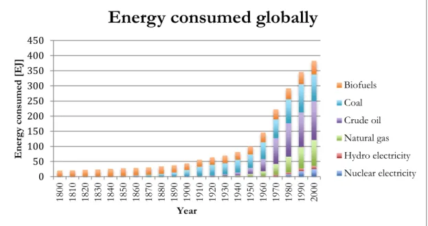
Graphic 1 explains this transition; the present information encompasses the energy consumed globally from each energy source from the 1800s to the 2000s. As can be seen at the global level, biofuel use has last longer than in England And Wales. By the 1700s coal accounted for about 50% of the energy consumed in these countries, while the same percentage in the world was only reached in the 1900s.

Graphic 1 - Energy consumed globally, by source [3]

But more important than comparing the discrepancies in energy transitions between the countries that started the industrial revolution and the rest of the globe is to focus on the most recent decades and on the energy consumption of the agricultural sector. Graphic 2 shows the evolution of the final energy consumption by sector in the EU between 1990 and 2014:

Graphic 2 – Final energy consumption, by sector [4] 0 50 100 150 200 250 300 350 400 450 1800 1810 1820 1830 1840 1850 1860 1870 1880 1890 1900 1910 1920 1930 1940 1950 1960 1970 1980 1990 2000 En er gy cons umed [ EJ] Year

Energy consumed globally

Biofuels Coal Crude oil Natural gas Hydro electricity Nuclear electricity

Graphic 2 shows that in recent years the total energy consumption in EU has declined and that the share of energy consumption due to agriculture is very small. Historically, the share of energy consumed by the sectors of: fishing, agriculture, forestry and others non specified has been small. Data from Eurostat shows that this share declined even more, from 4,22% in 1990 to 2,78% in 2014. However this tendency isn’t similar for all sectors, transport and services sectors have increased their energetic demand (although, recently, service sector has reduced this increasing tendency, and even began to reduce consumption) [4].

That being said, it is important to understand that in recent decades fossil fuels have been the dominant energy source which has led to several advantages but also brought negative points and nowadays with an increasing concern with the damage we have caused to the environment have been trying to reduce the pollutants emissions of fossil fuels as much as possible in order to preserve the planet's ecosystem.

With the objective above in view renewable energy sources are seen as the future because on the one hand they allow to preserve the planet and on the other hand unlike fossil fuels are inexhaustible energetic sources.

Thus, in this dissertation, the possibility of implementing a photovoltaic system in agricultural greenhouses will be studied in order to meet their energy needs, leaving the current vehicles powered with internal combustion engines and starting to use engines powered by the electricity produced locally.

1.2.

Objectives and methodology followed

The objectives of this project are mainly to develop a photovoltaic system to be applied in the production of electricity for agricultural greenhouses and if such work is feasible to optimize it in order to take advantage of the implemented system. For this the followed methodology will be:

1) Survey the energy needs of each energy-consuming equipment in the greenhouses in cause;

2) Processing the collected data constructing daily consumption charts distributed by equipment and by annual season;

3) Analyse various solutions of photovoltaic systems, from cell technologies, distributions and slope of panels, different peak powers, connection or not to the grid and storage or not of excess energy produced;

4) With the software PVsyst simulate various systems with the different characteristics exposed above;

5) Compare the simulated systems and choose the ones that might be more advantageous in cost/return prospects;

6) Moving towards the economic comparison of the simulated systems with the greatest potential and analyse their viability;

1.3.

Dissertation structure

This dissertation will be composed of six chapters.

The first will introduce work to be done, defining the framework and motivation by explaining the evolution of energy usage and effects fossil fuels have had on the world ecosystem, moving then to a more close analyse of the energy consumption in greenhouses. Also in this chapter, the methodology followed in this project was succinctly explained.

In the second chapter a literature review will be presented, having complete incidence on photovoltaic systems, defining them, listing the composing components, elucidating about technologies, project and assembly methods and constructive options, but also explaining the economic evaluation method.

The third chapter is all about the methodology followed in this dissertation. Beginning by extensively define the current problem/situation of the studied horticultural greenhouses, stating the data collected from visits done to these greenhouses and meetings with the farmers, define the expected characteristics for the photovoltaic system and explaining the design method.

Once the data is collected, in chapter four, energetic calculations will be carried on in order define the yearly energetic expenditures and to build an annual consumption model to define the photovoltaic system size. Additionally an analyse of the electricity and petrol prices evolution will be presented, first to define a price to use in future calculations but also for possible decisions on the implementation or not of the designed systems.

Finally, also in this chapter, will be defined some characteristics all the simulated systems will have in common i.e. cells technology, modules peak power, orientation, etc.

Chapter five will define the considered solutions, the built consumption model, results, viability of the solutions and possible optimizations.

The last chapter will summarize the obtained results, stating the conclusions, possible future work to be done in order to improve the results achieved in this work and some final considerations on which a personal point of view will be given.

2. Literature review

2.1.

Photovoltaic systems

2.1.1. Definition

A photovoltaic system is an energy production method that produces electricity using solar radiation that hits the earth. This method of energy production is possible due to PV cells which are made of semiconductor materials that absorb solar energy and convert it into DC electricity; in a PV system those cells are interconnected to form a PV module [5].

Besides the PV modules in a PV system there are other components, e.g. inverters, batteries, regulators, electrical components, mounting systems, among other minor components. For a better definition of the above-mentioned components, firstly the systems will be defined, in how they are connected, or not, to the electrical grid.

PV systems can be connected to the electrical grid, standalone or a mixture of both (hybrid system). Each of these systems has its characteristics, advantages and disadvantages, as well as the components necessary for its proper functioning.

Grid connected systems are characterized as the best cost/production option as with this kind of system there is no need in spending money in a vital but expensive component of off-grid systems: the batteries (which usually have to be replaced after about ten years) [6]. In addition, because this kind of system has the grid as backup electricity provider, when the system cannot provide the required electricity the grid will deliver the missing energy, which results in a lower peak power for the PV system as these peaks can be supplied by the electrical grid. Disregarding these peaks of energy it’s possible to diminish the system peak power, which results in a lower investment of capital in the beginning of the project.

As stated above, off-grid systems need batteries, this is a necessary component in this type of system since there will be periods in which there is more electricity being produced by the PV modules than it’s required, and without the batteries that energy would simply be lost. Moreover, the batteries also have an important role in delivering energy when there is not enough solar energy to be converted into electricity to supply the energetic demand. In this situations the batteries deliver the previously stored electricity assuring that there is energy to supply the consumer needs.

Consequently, while the grid-connected systems have the grid supplying the unfilled needs and absorbing the excess produced the off-grid systems have batteries. So with the grid-connected system every kWh of energy needed, that’s not possibly to obtain from the PV system, has a cost and every kWh of energy produced in excess will be sold to the

grid with certain compensation, while with the off-grid system the batteries will store and supply the excess and shortage of energy. This means that to choose between booth systems it’s necessary to weight the cost of the electricity and the cost batteries, but as well the compensation from the electricity sold.

Although there is a third option, the hybrid system that combines both systems above exposed. This system has the batteries as the standalone system does but it’s also connected to the grid as the grid-tied system is, with this solution it’s possible to reduce the cost of capital invested when compared with the off-grid solution as it’s possible to downsize the batteries capacity due to the support from the grid.

Now that the types of system connections have been defined it will be simpler to enumerate the components of each system, beginning with the grid-connected system. In this system, besides de PV modules, there are inverters and the mounting structure (which are common to all systems) and, besides some other minor constituents, there are no more components to be listed.

The off-grid system is more complex and in addition to the already mentioned components it also requires batteries, charge regulators and an optional generator.

Finally, the hybrid system requires all the equipments present in an off-grid system with the exception of the generator since this system is connected with the grid and any shortage of energy can be supplied by it.

2.1.2. Components

As stated before a PV system is composed of: PV modules, inverters and a mounting structure, and eventually of: batteries, charge regulators and generators. The PV modules have already been characterized in the last chapter so the definition of the PV systems components will be continued with the inverters.

The inverter has two functions in a PV system, first it has to regulate voltage and current coming from the PV modules, secondly it has to convert the DC electricity supplied by the PV modules into AC, which is used in most electronic equipments [6].

The mounting structure of a PV system is no more than a structure that keeps the PV modules in a position that can be: completely fixed (azimuth and tilt don’t change), with a rotation axis – in order to follow the trajectory of the sun during the day (changing the azimuth) or with two rotation axis following the trajectory of the sun changing both azimuth and tilt. The mounting structure can also allow the modules to receive the solar radiation concentrated, improving the electricity production.

Now that the modus operandi of the grid-connected system were described, lets move to the off-grid system.

Beginning with the batteries, as mentioned above store the electricity produced in excess and when that energy is needed they supply it, allowing the system to work even when there is lack or complete absence of solar energy [6].

Moving to the charger regulators, this component regulates the current delivered to the batteries in order to protect them from overcharging and maximizing their lifetime [6]. Finally, the generator, this is an optional component but usually present in off-grid systems as it will supplies the system energetic need when there isn’t sufficient solar energy to convert into electricity, allowing the battery bank capacity to be downsized as the system won’t be completely dependent on solar energy and therefore permits a reduction in the initial investment of capital.

2.1.3. Mounting type

Nowadays the possible mounting types of a PV system are: rooftop, facade or ground-mounted. Each type of mounting has its advantages and disadvantages, that will followingly be presented.

Beginning with the advantages of the roof and facade-mounted systems, the main upside of this systems is the space optimization possibility since the roofs and facades of the buildings usually aren’t used and by installing the PV modules on them allows other spaces to be used for other proposes. Moving to the advantages of ground-mounted systems, with this type of mounting the maintenance and cleaning of the PV modules is simplified and there is the possibility of expanding the primary system, which on a rooftop might be harder due to lack of free space.

Now the disadvantages of each mounting method, with roof-mounted systems there is the need of either having a flat roof or having the roof north/south faced since that is the direction that allows a better performance for the PV modules, roof surroundings creating shadings in the places where the PV modules could be mounted and rooftop obstacles in the way. The facade-mounted system has a similar problem since the building facade has to be north/south faced or the PV modules performance will be reduced. In the case of ground-mounted systems the main disadvantage is the occupation of space that has to be bought or that could be used with other purposes.

2.1.4. Tracking method

As it’s commonly known every day the sun rises in the east and sets in the west, during this period its height changes, having its lower height during the sunrise and the sunset and peaking the height around the midday. For PV systems dimensioning this is an important information as the PV cells produce more electricity if the hitting radiation is more intensive, with that in mind it’s desirable to orientate the PV modules in order to have the sun light hitting the panels as close as possible of the 90 degrees – inclination that maximizes the PV cells electricity production.

That being said there are two types of tracking methods, they are the single-axis system and the dual-axis system. In the first case, the single-axis system the PV modules are

rotated following the sun path during the day, this is the PV modules change its azimuth, in order to have the sun light hitting the PV panels as close as possible of that desirable angle of 90 degrees. The dual-axis system, used in the concentrator PV, also changes the PV modules azimuth following the sun path from its rise until it set but also changes its tilt assuring that the desirable angle of 180 degrees between the sun light and the PV panels is even closer than with the single-axis system.

Those are the two tracking methods currently available but there is a third option that is not having a tracking system, with this option the PV modules are fixed and an orientation and tilt that grants the better output from sun energy conversion are calculated and the PV modules are installed accordingly.

2.1.5. Photovoltaic cell technologies and efficiencies

The photovoltaic cells are the main component of the PV modules having an important role into the energy conversion process and therefore should be carefully analysed. This component has been developed through three generations, in the first the PV cells were only based in crystalline silicon (c-Si), the second generation also included thin-film technologies and with the third generation the concentrator photovoltaics (CPV) came [7]. With each development of PV technologies, more building options were available for the cells, followingly each generation will be more carefully analysed.

The first generation of PV technologies can be sub-divided into three different cell-building materials, the monocrystalline silicon (mono c-Si), the polycrystalline silicon (poly c-Si) and the ribbon silicon (ribbon c-Si). With the second generation came the thin-films that can be built of amorphous silicon (a-Si), multi-junction thin silicon film – also known as amorphous/microcrystalline silicon – (a-Si/μc-Si), cadmium telluride (CdTe) or cooper indium gallium (di)selenide (CIGS).

Finally, the third generation marked the appearance of the concentrator photovoltaic, which is a technology that uses lenses to concentrate solar light into the PV cells increasing the intensity of the light hitting the cells. This technology uses single junction cells, typically made of gallium arsenide (GaAs) or III-V multijunction cells to fit the PV modules. Besides the CPV technology, the third generation also brought organic photovoltaic cells (OPV) and hybrid die-sensitised cells (DSSC) which are considered very promising technologies [7, 8].

Now that each PV cell technology has been exposed it would be good to compare these solutions in order to discover their advantages and disadvantages. In the following graphic it’s shown the evolution of the efficiency of each cell technology.

Graphic 3 – Historic efficiency of solar cells (higher scores from the lab) [9]

As it’s shown in graphic 3 the third generation cells building materials reach the higher efficiencies closely followed by monocrystalline silicon cells and then came the polycrystalline silicon cells, cooper indium gallium (di)selenide cells and cadmium telluride cells that have all similar efficiencies.

So if the choice was to be made only by cells efficiency the obvious choice would be III-V multi-junction cells since they would allow more electricity production than any other cell type as well as save in space needed for the PV modules. However the choice is not so linear because these technologies have different costs, lifespans and maintenance requirements.

Currently the market leader is, and by a huge distance to the other solutions, the crystalline silicon cell. In graphic 4, on the right, is shown the historical data and expectation of evolution of the PV cells market and as it is visible the crystalline silicon (c-Si) has since the beginning dominate the PV cell market with always more than 60% of the market share. However, as we can observe since the 2005s the tendency is to reduce this share and open space for the other technologies to be more seek and therefore to have more developments.

Graphic 4 – Historical data and expectation of evolution of the PV cells market (in percentage) [7]

2.1.6. Economic evaluation method

A PV system to be applied in real situations has the final objective of giving profit to the user, this is: to allow the user to save money during the system operational years, for that a research will be done in order to have data to compare with the obtained values to define if the designed system is viable or not. This research has the objective of providing data, calculation methods and price evolutions for the balance of system (BOS), PV modules cost, inverters cost, total system cost, energy cost, payback time and levelized cost of electricity (LCOE). In the following chapters the information collected in this research is shown.

Balance of system (BOS)

The balance of system (BOS) incorporates all the costs of the equipments composing a PV system, exception for the modules and inverters. Followingly these equipments are listed [10]:

 Hardware

o Cabling: All AC (only low voltage) and DC components, such as cables, connectors and combiner boxes;

o Mounting: The complete mounting of the system, including foundations and material for the assembly;

o Grid-connection: All medium voltage components, switch gears, transformers and meters;

o Control: Monitoring system, meteorological software, data system; o Safety and security: Camera system, fences, anti-theft equipment.  Installation

o Mechanical installation: Access roads, uploading and transport of the equipment, preparation for cable and installation of the system;

o Electrical installation: Installation of cables and control system; o Inspection: Construction supervision, health and safety inspection.  Soft costs

o Permitting: Costs related to necessary permits for the construction and operation of the PV system;

o System design: Costs due to design of the system, geological surveys, structural analysis and necessary documentation;

o Customer acquisition: Costs for projects rights, provisions paid to get the project and off-take agreements;

o Financial costs: Financial costs necessary for development and construction of the project;

o Incentive application: Costs related to the appliance to benefit from support policies;

o Margin: Profit margins for the engineering company and the project developer.

Having defined the costs composing the BOS, in graphic 5 is exposed the BOS cost (for utility scale systems) for some countries in 2015.

Graphic 5 – PV BOS cost in 2015 [10]

Modules cost

PV modules prices have been experiencing an effect called price experience curve, this effect is characterized by the decrease of a technology cost by a certain percentage every time the cumulative produced volume doubles. This effect was first described by Wright and later generalised by Henderson of the Boston Consulting Group (BCG). The following graphic represents the evolution of PV modules prices between 2010 and 2016, as well as the average prices in 2015 for some countries [9].

Graphic 6 – Evolution of prices of PV modules between 2010 and 2016 [10]

In graphic 6 we can see the decline of around 80% in PV modules prices between 2010 and the end of 2015.

Inverters cost

Inverters, like PV modules also have been experiencing the price experience curve effect, showing a learning rate of about 19%. Currently the inverters prices are between 0,38 USD/W for micro-inverters (module power range) and 0,14 USD/W for central inverters (for power conversions above 100 kWp), being the string inverters (with up to 100 kWp of power conversion) in the middle of that price range with a cost of around 0,18 USD/W [9, 10].

Batteries cost

Standalone systems require an energy storage method, which can come in various forms, i.e.:

 Mechanical storage: Pumped hydro storage (PHS), compressed air energy storage (CAES) and flywheel energy storage (FES);

 Thermal storage: Molten salt energy storage (MSES), phase change materials and hot-water;

 Chemical storage: Hydrogen, synthetic natural gas (SNG), other chemical compounds;

 Electrical storage: Supercapacitors (SC) and superconducting magnetic energy storage (SMES);

 Electrochemical storage: Sodium-sulfur batteries (NaS), vanadium redox-flow batteries (VRB), lead acid batteries (PbA), lithium-ion batteries (Li-ion), among others [11-13].

PV systems utilise electromechanical storage, this is: batteries to store the excess of electricity produced by the PV modules. Graphic 7 shows the maturity of some storage technologies, as well as the need of investment to develop them to the predicted level since 2011 until 2020.

Graphic 7 – Maturity level of storage technologies [12]

Lead acid batteries, lithium-ion and flow batteries are the important technologies, as they are the used in PV systems.

Flow batteries are the ones that need more investment in research and development and at the same time the less developed.

Lead acid batteries, currently, are the more advanced in terms of development, however to keep progressing will need more investment than lithium-ion batteries.

When it’s necessary to choose the type of battery to use in a system there are some factors to take into account, as: efficiency, number of cycles during the battery lifetime and cost. The following two graphics show the efficiency and number of cycles a storage technology is able to do during its lifetime.

Graphic 8 – Efficiency of storage technologies [11]

Graphic 9 – Number of cycles of storage technologies during their lifetime [11]

The costs per kilowatt-hour [$/kWh] of storage technologies, for the three important technologies (Li-ion, PbA and flow), are the following:

 Lithium-ion: Between 200 $/kWh and 1000 $/kWh;

 Lead acid and advanced lead acid: Between 400 $/kWh and 700 $/kWh;  Vanadium flow: Between 600 $/kWh and 1200 $/kWh;

Total costs

The cost of a PV system includes the total costs of all the components composing the system, and therefore can be divided in the BOS, modules and inverters costs. Graphic 10 shows the evolution of the total cost of gird-connected utility-scale systems between 2010 and 2015.

Graphic 10 – Evolution of the average price of PV systems between 2010 and 2015 [10]

System cost per kilowatt-peak

A PV system has a wide range of prices and energetic outputs, depending on factors as the type of system (grid-connected or standalone), system power peak, chosen technologies, system localization, tracking method, among others. To compare different solutions in terms of cost per kilowatt-peak, a calculation involving the total initial investment and the system peak power is done. Equation 1 expresses the calculation method:

System cost per kilowatt– peak = Total system cost System peak power

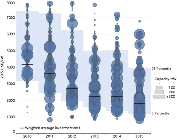
The above equation provides a value [€/kWp], with which different systems can be compared in terms of investment by installed peak power and which allows to understand if the cost of the system is common in the market, for the installed power. Graphic 11 shows the evolution of cost of utility scale PV systems between 2009 and 2025 and will be used as comparison method to define if the cost per kilowatt paid for the systems simulated is acceptable.

Graphic 11 – Evolution of the cost of utility scale PV systems between 2009 and 2025 [10]

Payback time

While the system cost per kilowatt-peak allows the comparison and evaluation of systems through cost of the system by installed power, the payback defines the time (years) that the system will have to operate to pay it self. The following equation express the payback time calculation method:

Payback = System initial cost

Annual savings with PV system

With this equation is possible to evaluate the time a system takes to begin to be profitable, and decide if it may be viable. The annual savings from the above equation are calculated according to equation 3:

Annual savings with PV system =

= Expense on energy without PV system − Expense on energy with PV system

Eq. 3

And the energetic expenditures are determined according equation 4 and 5:

Expense on energy without PV system =

= Vehicles consumption × Petrol cost + Electric consumption × Electricity cost

Eq. 4

Expense on energy with PV system =

= Electricity bought from grid × Electricity cost −

−Electricity injected into grid × Compensation for the electricity sold

Eq. 5

As some of the above parameters change over time, to calculate the annual savings some considerations had to be made, they were the following:

 The energetic needs of the greenhouses were considered constant over the operating life of the PV system;

 The electricity produced by the PV systems will decrease every year, this happens due to the degradation of the systems, in future calculations a degradation factor of 0,5%1 _{will be considered;}

 The cost of energy tends to rise, so an annual increment in the cost of petrol and electricity will be considered.

1 _{Literature doesn’t provide a definitive value for the degradation factor as it depends on}

numerous variables. More data about this value may be found in NREL report from 2012 about Photovoltaic Degradation Rates [15]

Performance ratio (PR)

PVsyst automatically calculates the system PR. This parameter defines the ratio between energy effectively produced and the energy that could be produced if the system operated continuously under STC. The PR is included in PVsyst report and includes both, system and array losses [16]. This parameter is calculated according to the following equation:

PR =Yf Yr× 100

Eq. 6

The variables in the above equation have the following meaning: Yf – Daily useful energy (system yield);

Yr – Ideal array yield, system production disregarding losses. Value equal to the incident energy in the modules plane.

Levelized cost of electricity (LCOE)

Due to the drop of PV components cost allied with the rising of energy prices the LCOE for PV systems has also suffered declines. Graphic 12 expresses the evolution of the LCOE for residential systems in some countries between 2006 and 2014.

If the cost evolution of PV modules and the LCOE (graphic 6 and graphic 12) are compared it’s possible to detect similarities in the curves evolution, that happens because the LCOE and the PV modules prices are linked as the following equation demonstrates [18]. LCOE =∑ It+ O&Mt+ Ft (1 + r)t n t=1 ∑ Et (1 + r)t n t=1 Eq. 7

The variables in the preceding equation mean the following: It: Investment expenses in year “t”;

O&Mt: Operations and maintenance costs in year “t”;

Ft: Fuel expenditures in year “t”;

r: Discount rate; t: Year;

Et: Amount of electricity produced in year “t”;

n: Operational life of the system.

From the equation above is possible to conclude that with the increasing of the investment expenses (PV modules, inverters and BOS), operations and maintenance and fuel expenditures the LCOE increases. In opposition is the generated electricity that reduces the LCOE if it’s increased.

Having already defined what the investment expenses are, let’s now analyse the operations and maintenance in a PV system. In the beginning O&M costs didn’t have a major contribution for the LCOE of a system as it’s value compared with the other costs was diminutive, however with the declining of the PV modules and inverters prices a new reality came and the share of O&M in the LCOE increased significantly. In 2014 O&M costs already accounted for 20% to 25% of the LCOE in countries like Germany or United Kingdom, being that 45% of the O&M costs were maintenance costs, 18% land lease, 15% local rates or taxes, being the lacking 22% distributed by a variety of other factors [10]. In future calculations the O&M cost, in the first operational year of the PV system, will be 1% of the total initial cost of the system, being considered an increment in the O&M cost of 2% per year [19].

Moving to the fuel expenditures, considering that the LCOE is going to be calculated for a grid-connected PV system or an off-grid without backup generator, this variable will be equal to zero.

The discount rate is an economic term that represents the rate to be applied in a calculation to determine the value a future amount of cash has today.

Finally, the electricity produced depends on the system (peak power), as well as the conditions (meteorological and positioning) of the site in which the system is going to be installed and the degradation factor considered that will decrease the electricity produce every year.

3. Methodology

In this chapter will be explained the current problem/situation of the greenhouses and the prospect of work to be realized, to do so the information obtained from two visits done to greenhouses, as well as information obtained from the cooperation of the farmers by handing other important that could not be collected on the field and an operation of measurement of the electricity consumption on the greenhouse will be fundamental.

With the information acquired the current working methods will be stated, as well as energetic needs and existing technology. After the problem is defined the characteristics the system must meet will be presented but also the method of design taken in account.

3.1.

Definition of the problem/situation and prospects for the

project

The objective of this project is study greenhouses operation methods and energetic needs in order to project possible solutions to optimize the energetic expenses and costs. Currently the pumping system and all other electricity consuming equipments use electricity bought from the grid, while the vehicles that make the vaporization of the crops are powered by combustion engines.

The pumping system has to work when “the crops demand”, this is when the crops can absorb more water, so the system is autonomous – but can be remotely activated if necessary.

The vehicles operating periods are not entirely defined but their usage is, more or less, continuous.

After the definition of the situation the work will go through the definition of some hypothesis for the system and simulation of those hypothesis, once the simulations are done the work will proceed by comparing the results with each other and with the costs of the actual system in order to define if there is any viable solution.

3.2.

Visit to greenhouses and data collection

As stated above the first stage of this work was to get information on the greenhouses working methods as well as collect information about the energy needs and distribution and the current technology and machinery. So in order to compare information, two visits were done.

From the first visit to the greenhouse the following aspects were collected:

 Currently the greenhouses operations are made by two petrol moved vehicles with 6 hp of power each and with each one working an average of two hours a day;

 In critical days both vehicles must work 7 to 8 hours;

 There has been no major maintenance problems with any of the vehicles;

 There are two pumps, one with 1 hp to pump the water from a hole to a reservoir and another with 7,5 hp to water the plants with the water stored in the reservoir;

 The watering hours cannot be controlled since it has to be done when the plants need, typically when the sunrises;

 The morning watering usually takes around two hours to be done;

 There is more electricity consumption during the summer due to longer watering periods;

 The farmers can control the watering times, beginning and ending from anywhere since there is a control system that can be operated via wi-fi using a mobile phone;

 The fields where the greenhouses were built usually have some empty ground were PV modules can be installed if needed.

From the second visit some contradictory information was collected but also important information about that year lettuce demand (which composed the majority of that greenhouse plantation), about the contradictory information:

 The watering doesn’t necessarily has to be when the sun rises, the given information points to two to three waterings per day;

 The watering doesn’t necessarily has to be two hours long, it can take for example four or five hours divided by two or three waterings.

And the information about the lettuce demand:

 From some months ago the demand of lettuce has drastically dropped causing the plantations to be directly thrown away, because of this those plantations haven’t been getting so much water and so the readings (measurement of the greenhouse electricity consumption that will be explained next) might not be the common reality for that time in the year.

Besides the data collect along with the farmers there was also a measurement of a greenhouse electricity consumption during an entire month, which clarified the monthly electric consumption as well as its distribution.

That measurement, besides the monthly electric consumption profile also permitted to correct the power considered for the watering pump as the pump nominal power given by the farmers was 7,5 hp (approximately 5,6 kWh) and this value only was reached or overtaken a few times during a month, which meant that the pump power should be lower since these kind of equipments usually worked at their nominal power or at least close of it.

That correction had to be done because in the distribution of the electric needs the equipments will be considered to always be working at nominal power.

For the vehicles yearly consumption a file was handed on which was specified the diverse fuel consumptions during a year.

In the end the pumps and other electricity consuming equipments consumption in April was 462,664 kWh while the yearly petrol consumption was 1656,50 l.

At this point is necessary to explain that it was impossible to acquire annual information about the electricity consumption, so in future calculations monthly consumptions will be constructed knowing the electric consumption in April.

3.3.

Characteristics the system must meet

After the visits and the electricity consumption measurement was done the data collected had to be treated in order to define the different consumptions and its distributions, to do so the following considerations were made:

 There will be two vehicles and the vehicle’s working days are five a week;

 Each vehicle will have 2,7 kW of nominal power (power defined by green^2, company responsible for the choice of the vehicles and their power);

 During four of the five weekly working days only one vehicle will be considered working at time;

 On the other working day both vehicles will be considered working simultaneously;

 The watering will be considered starting when the sun rises and will have different durations and hourly energetic consumptions;

 Also the hourly energy consumptions were calculated considering the equipments (vehicles, pumps and others) always working at their nominal power.

In chapters 4.1. and 4.2. the electric needs of the vehicles and pumps and other electricity consuming equipments will be shown allowing a better understating of the considerations taken into account.

3.4.

System design method

Once the necessary data had been collected, and treated, and some parameters had been defined (topic approached in following chapters) the calculation process could begin. The calculation process will be carried by the photovoltaic software PVsyst [16], this is a very complete software and allows the acceleration of the systems calculation time. Opening the software it immediately displays a window on which it’s possible to begin the project design and choice between the following four types of systems:

grid-connected, stand alone, pumping and DC grid. For this project only the first two options will be simulated as the there wasn’t enough data to define the pumps consumption and the DC grid option is to be applied to public transport networks.

Once the system type is defined a new window will be displayed and in this the project has to be defined, the first requisite is to choose the geographical location of the system: country and geographical site, if the geographical site and corresponding meteorological file are available in PVsyst database, then the software automatically defines the meteorological file, however if the meteorological file is not available in the software database, then there are three options:

1) Standard procedure:

 The standard procedure used by PVsyst in these situations is to automatically create a synthetic hourly file with the monthly data of the site.

2) Customizing a site:

 Select the nearest site with corresponding meteorological data available in PVsyst database knowing that using this method there will be an error associated that will be as bigger as further apart the two sites are;

 Choose a different site and change it’s coordinates (no more than 2º) so the software takes those changes into account and creates a new meteorological data file.

3) Create a meteorological data file:

 Select the correct site and build a new monthly meteorological data file. Having defined the system geographical site and meteorological data is possible to define the PV modules orientation (azimuth and tilt), for that a new window opens on which besides the orientation it’s possible to choose the system tracking method and how the optimization will be calculated – yearly irradiation yield, summer yield (April to September) or winter yield (October to March), with each change the software automatically calculates the yearly meteorological yield presenting the transposition factor (ratio between the incident irradiation on the defined plane and the horizontal irradiation), loss by respect to optimum (shown in percentage represents the module yield loss due to the chosen tilt when comparing to the optimum tilt) and the global irradiation on collector plane (value presented in kWh/m2 _{represents the yearly}

production of a PV module in the defined orientation per square meter of module). Using this software the PV modules orientation is made much easier since with any change the software automatically does all the calculation and even compares to optimum values.

After the system orientation is chosen, it’s possible to define the system. For that a new window is displayed in which the first phase is to size the system, this is either selecting a power for the system, available area to install PV modules or else no sizing.

After this information is given, in the same window is displayed a list of PV modules – list that can be updated with PV modules chosen by the user – from which the desired modules must be selected. Once the modules are selected, if a power has been chosen or

the available defined, the software automatically calculates the number of approximated modules needed.

Until this point the methodology was the same independently the system being connected to the grid or off-grid but the next is different, if the system is connected to the grid then an inverter has to be chosen, if the system is off-grid then it’s the batteries that have to be chosen.

So considering first a grid-connected system, the next step is to choose an inverter that can correspond to the system needs (operating voltage), for that another list is shown but that with all the inverters in the software database – this list also can be updated with other inverters.

Once the above variables have been selected PVsyst automatically defines an array alignment, distributing the modules in strings and series. However it doesn’t mean that the designed array can’t be changed, actually the user has freedom to arrange the array at wish, for that the software even defines the maximum and minimum number of recommended PV modules – depends on the chosen inverter – that can be put in each string and in series.

After all the requirements listed above are fulfilled the software shows the operating conditions, the array nominal power (STC), number of modules and area used.

Now considering an off-grid system, for this kind of systems the first things to define are:

 Loss-of-load (LOL) probability, this variable defines the probability of the user needs couldn’t be supplied because of batteries low charge [16];

 Autonomy: number of days the system can supply the user needs without any solar radiation being converted into electricity considering the battery bank starting with full charge;

 Battery bank voltage: voltage for which the battery array will be designed. Once those parameters are defined and the modules chosen it’s necessary to choose the batteries, for that once again a list of available batteries in the database is displayed. After the choice has been done the software immediately calculates the amount of batteries needed, depending on the LOL probability and number of autonomy days, and distribute them by series and parallel depending on the desired voltage.

After the batteries have been chosen the regulator must be selected, for that another window is shown on which the list of regulators of PVsyst database is displayed (regulators can also be added to PVsyst database), when choosing this component the vital part is assure that charging voltage comprehends the array output voltage.

As in the grid-connected system, once all the requirements are fulfilled the software shows the operating conditions, the array nominal power (STC), number of modules and area used but also the nominal capacity of the battery bank.

In the window were the system is defined is still possible to define two more aspects: user needs and the system losses.

Beginning by exploring the user needs window, to define the energetic needs in PVsyst the user has the following options:

 Build a daily household consumption model with an interface that shows common household equipments and that needs to be filled with the number of equipments of each type, this model can defined as constant over the year, seasonal or monthly;

 Select a fixed constant load that will be used every day, all year long;

 Define monthly values: monthly average consumptions that will be used by the software as constant during each month;

 Daily profiles described by hourly consumptions that can be defined with one of the following distributions:

1) Constant during the year, meaning each day will have the same hourly consumption distribution;

2) Seasonal profiles, meaning that four seasonal averages have to be calculated so the software uses each of those averages as constant values during the corresponding season2_;

3) Monthly normalisations, one daily profile is defined and then his amplitude is modulated according to given monthly values;

4) Weekly modulation, two daily profiles – constant over the year – are defined, one for “working days” and other for “week-ends”.

 Probability profiles, as this consumption distribution is more suited for DC-grid systems won’t be approached here;

 Distribution externally loaded: import a consumption distribution from extern sources.

Finally, the last aspect that can be modified from this window: the array losses, PVsyst defines six classes of losses:

 Thermal losses: To calculate thermal losses PVsyst uses the following equation:

U = Uc + Uv × v Eq. 8

The factor U represents the thermal loss [W/m2_{K], the factors Uc [W/m}2_{K] and}

Uv [Ws/m3_{K] are split components of the thermal losses that represent a}

constant component and a component proportional to the wind velocity, respectively.

There aren’t defined values for the variables above but the software has 20 W/m2_{K defined for the the factor Uc and 0 W/m}2_{K/m/s for the Uv factor as}

default [16];

2 _{Season distributed as follow: Summer (June-August), Autumn (September-November),}

 Ohmic losses: The wiring ohmic losses represent the losses from the power available from the modules and the power available at the end of the array. PVsyst automatically defines 1,5% as wiring loss fraction with respect to the STC. However the software has a tool that does the optimization (determination of the wires cross section) of the wiring losses, for that the average length of wires between string module connexions, and between the inverters and the main box are required. In this separator is still possible to calculate the losses between the output of the inverter and the injection point, for that Pvsyst requires the wiring length, and due to external transformers [20];

 Module quality: In this separator three losses can be defined – module efficiency loss that reflect the deviation of the average effective module efficiency by respect to manufacturer specifications, Pvsyst recommends this value to be half of the lower tolerance of the modules [20].

Light induced degradation (LID) represents the degradation of crystalline silicon modules, during the first operational hours by respect to the manufacturing flash test STC values, Pvsyst recommends as default a value of 2,0%;

Mismatch losses define the losses due to modules with different characteristics, i.e. different current or voltage, being the string current equal to the module with lower current. For this loss in particular PVsyst allows more detailing, i.e. definition of the groups of cells or modules, external conditions and other parameters that cause mismatching [20];

 Soiling loss: This separator allows to define losses due dirty covering the PV modules, being possible to define a global or monthly percentages;

 IAM losses: The incidence loss is sufficiently well defined by Ashrae and theoretically won’t have to be changed [20];

 Unavailability: In this separator is possible to define the yearly time the system will be unavailable and the number of periods on which that time will be distributed (the distribution can be automatically generated by the software or manually defined).

Having defined the system is possible to define some more aspects to improve the results from the simulation. The definition of the shadings in the modules go through two phases, close shadings (near shadings) and far shadings (horizon).

The horizon should be considered for distances equal or superior of twenty times the PV array size and can either be defined using a solar chart in which the shades are drawn or by importing a file from an external source [16].

The near shadings change during the day and over seasons and define this parameter is one of the most difficult process in the software and won’t have a detailed explanation in this project as this tool won’t be used [16].

To define the near shadings in PVsyst a 3D construction has to be built which allows the software to define the shadings.

The final stage of the system design is the module layout, however in this version this tool is only descriptive, having no interest for the simulation [16].

Once the system is designed the software unlocks the simulation (to run the simulation the parameters that have to be defined are: meteorological site, user needs – in form of distribution, available area or system peak power, orientation, tracking method, PV modules, inverters and, for standalone systems batteries and regulators), running the simulation PVsyst automatically generates a report and a set of tables to evaluate the system.

4. Greenhouse energy needs, distribution and cost

The main energy consumption in these greenhouses is due to vehicles, which are powered by petrol, and the pumping system, which are electricity-consuming equipments. The first phase in the calculation of energy needs is conversion of the collected data about the vehicles consumption, which was given in liters of consumed petrol and convert it to tonnes of oil equivalent (toe), so after it’s possible to obtain the equivalent consumption in kWh.

After the vehicles equivalent consumption is calculated, the consumption of the electricity consuming equipments (which includes the pumps) will be defined, to do so the data collected during the month on which the readings were realized will be analysed.

4.1.

Calculation of vehicle consumption

To convert the given consumption, in liters, to kWh there are some reference values and conversion factors that have to be taken in account. They are the following:

 Petrol density: 0,75 t/1000 l;

 1 t of petrol is equivalent to 1,073 toe [21];  1 toe is equivalent to 4651,163 kWh [22].

Note that the 4651,163 kWh per toe already take into account 40% average EU generation efficiency, otherwise the value would be 11627,909 kWh per toe, which would mean that for the same petrol consumption the electric need would be two and half times bigger.

After the reference values and conversion factors were established the subsequent calculations were done:

Fuel consumption (t) = Fuel consumption (1000 l) × Petrol density (t/1000 l) Eq. 9

Fuel consumption (toe) = Fuel consumption (t) × 1,073 Eq. 10

Electric consumption (kWh) = Fuel consumption (toe) × 4651,163 Eq. 11

The above calculations resulted in a final yearly electric consumption, for the vehicles of 6200,318 kWh, beginning with a fuel consumption of 1656,50 l of petrol per year.

4.2.

Calculation of pumping consumption and others

Values obtained from measurements done on the greenhouse allowed to determine the electric consumption of the greenhouse. However, to obtain that value a calculation had to be done, as the measurements were done with time intervals of five minutes, to determine the electric consumption of a period the absolute value of that period had to be subtracted from the previous value.

On a first stage all the values registered will be considered and with them daily graphics of the electric power peaks distribution will be built, those graphics will allow to the rectify the values of the nominal powers of the pumps.

Because the graphics show the peaks of power between time periods of minutes it was possible to have an idea of the power of the electricity-consuming components (knowing that there were to pumps but also other components that consumed electricity e.g. the opening and closing system of the greenhouses), with that in mind was hard to believe that there could be a pump with a nominal power of 5,6 kW when the data was analysed as that value almost never was reached and barely approximated during that month, actually the power peak values usually were either 3,5 or 5 kW, therefore in order to create an annual distribution as similar as possible to the real distribution two pumps were considered, one with 3,5 kW replacing the 1 hp pump and another with 5 kW replacing the 7,5 hp pump, being other equipments disregarded since with the considered power for two components above a close approximation was achieved.

Besides the pumps power, it’s also necessary to define the model of energy consumption in the greenhouses. From the readings of power peaks it’s possible to identify a tendency of power usage between around 6:00 am to 10:00 - 11:00 am.

However that is not always the scenario, there were days on which there was power need on the dawn, between 3:00 am to 9:00 am and also days on which the power consumption occurred in the afternoon, in this case with completely random distributions. So to build the distribution of consumption, the data collected along with the farmers that stated that usually the plants need more water when sun rises came in hand and the distribution was done so the watering begins when the sun rises.

As for the duration, different periods were considered, depending on which season the watering was being done, for example, during the winter the watering would take four hours and during the summer it would take five hours. Lastly, also the power used for the pumping changed with the season, if in the winter the considered power was 3,5 kW, in the summer the utilised power increased to 5 kW. Autumn and spring were mid-term seasons between the colder and wetter and the hotter and drier season.

One final note about the seasons beginning, in this model it was considered that each season starts at the beginning of the corresponding month so for example in the case of the summer that begins on June 21, in this model the consumption hours were changed on June 1.