2019
UNIVERSIDADE DE LISBOA
FACULDADE DE CIÊNCIAS
DEPARTAMENTO DE BIOLOGIA ANIMAL
Spatial patterns of genetic diversity in Hyla molleri
Patrícia Cruz Gonçalves Guedes
Mestrado em Biologia da Conservação
Dissertação orientada por:
Doutora Ana Veríssimo
Doutor Carlos Fernandes
iii
Agradecimentos
À Ana, à Sílvia e ao Guillermo, os meus orientadores no CIBIO e os investigadores que
tornaram possível o desenvolvimento desta tese. Obrigada por toda a paciência que
demonstraram neste caminho cheio de curvas, e por todos os ensinamentos que me
deram ao longo destes meses. Agradeço imenso a oportunidade que tive de expor o meu
trabalho sob formato de poster no “Evolution” em Agosto passado, foi uma experiência
incrível. Sinto que aprendi muito com esta tese, não só a nível de desenvolvimento de
trabalhos científicos mas também sobre mim mesma e devo-vos isso.
Ao Professor Carlos, por ter sido sempre um orientador interno interessado no progresso
da minha tese e por me ter ajudado em diversas ocasiões, mostrando-se sempre
disponível.
Às quatro raparigas que foram a minha rocha neste percurso: a Carolina, a Patxó, a Sara
e a Tânia. Sem vocês não sei o que tinha sido de mim ou desta tese. Obrigada por terem
sido o melhor grupo de apoio que alguma vez poderia ter pedido, celebrando as minhas
vitórias e ajudando incansavelmente nos momentos difíceis. Esta tese é minha, mas não
a teria feito sem vocês. Não conheço palavras que expressem o quanto gosto de vocês e
o impacto que têm na minha vida. Obrigada.
À Cata, por me ter acompanhado em todas as alturas desta viagem. És das melhores
pessoas que conheço e agradeço muito estares na minha vida. Mereces uma medalha por
me aturares.
Ao José e à Joana (Zé e Jú, vá), pelo apoio incondicional que têm demonstrado ao longo
dos anos de amizade (e já lá vão muitos!), reforçado ao longo deste percurso. Sem o
vosso incentivo e incansável fé em mim não sei onde estaria. A vida sem vocês não
seria a mesma.
Por fim, quero agradecer à minha família, sem a qual nada disto teria sido possível. Não
só me apoiam incondicionalmente, como acreditam em mim quando eu não o faço.
Obrigada por tudo o que têm feito por mim. Não poderia ter família melhor.
Esta tese fez-me crescer muito. A nível profissional, claro, mas também a nível pessoal,
permitindo-me compreender as minhas capacidades, força e limites. Mas acima de tudo
mostrou-me que estou rodeada de pessoas incríveis e que estão presentes nos bons e
maus momentos. Foi uma viagem acidentada, mas valeu a pena. Estou ansiosa pelo
futuro.
Este trabalho foi financiado por Fundos FEDER através do Programa Operacional
Factores de Competitividade – COMPETE e por Fundos Nacionais através da FCT –
Fundação para a Ciência e a Tecnologia no âmbito do projeto
PTDC/BIA-BIC/3545/2014.
v
Resumo alargado
A diminuição acentuada das populações de anfíbios a nível global é uma das maiores preocupações de conservação da Natureza da actualidade. De facto, a União Internacional para a Conservação da Natureza (UICN) classifica 41% das espécies de anfíbios como ameaçadas de extinção, o que torna este grupo num dos mais ameaçados do planeta. Apesar de se conhecer os factores de ameaça dos anfíbios (p.e. perda de habitat, alterações climáticas, quitridiomicose, etc.), ameaças como baixa diversidade genética, aumento da deriva genética e endogamia tem sido largamente ignoradas.
A diversidade genética é produto da diversidade alélica e genotípica encontrada na espécie e, de acordo com a UICN, é um dos três níveis de biodiversidade que necessita de medidas de conservação. Por ser a base do potencial evolutivo das espécies, a diversidade genética é fulcral para a capacidade que uma espécie tem de ultrapassar alterações no fitness populacional, actuando como uma salvaguarda no caso de redução significativa da população face a um evento catastrófico.
A diversidade genética pode ser classificada em duas categorias: adaptativa ou neutral. A primeira está sob a influência de forças selectivas e confere maior fitness nas condições em que a espécie se encontra; a segunda não está sob a influência de forças selectivas e permite inferências sobre processos demográficos. Em estudos de conservação, o foco tem sido sob a diversidade genética neutral, maioritariamente para a definição de Unidades de Conservação dentro das espécies.
De um ponto de vista genético, as populações de anfíbios têm reduzido efectivo populacional, que se traduz num baixo número de indivíduos reprodutores, e estão mais propensas a fenómenos de deriva genética e redução de diversidade genética. Várias características do habitat, tais como a elevação ou distância geográfica, podem também impactar a diversidade genética dos anfíbios, actuando como barreiras ao fluxo de genes devido aos gastos energéticos associados à deslocação entre locais. A baixa capacidade de dispersão aliada às necessidades de habitat (como elevada humidade atmosférica), limitam a conectividade entre populações e levam a um aumento da deriva genética. Adicionalmente, a história biogeográfica da espécie pode também desempenhar um papel importante na diversidade genética: em anfíbios, os padrões de diversidade genética aparentam ser mais fortemente moldados por acontecimentos históricos do que por fenómenos recentes, com a maioria dos taxa mostrando múltiplas linhagens de ADN mitocondrial estruturado geograficamente. Mais especificamente, foi o período de glaciações do Pleistoceno que profundamente alterou a distribuição das espécies, através de repetidos acontecimentos de extinções locais, concentração em áreas de refúgio, e nova expansão a partir desses locais, levando a uma forte estrutura genética e divergência entre populações.
A genética da paisagem invoca um design de amostragem focado em características da paisagem e no uso de ferramentas genéticas e estatísticas para identificar padrões de diversidade genética que possam ser explicados por uma ou várias características ambientais/da paisagem. A paisagem pode influenciar os padrões genéticos de uma espécie por principalmente dois processos: isolamento-por-distância e isolamento-por-ambiente. No isolamento-por-distância, é o aumento da distância geográfica que impulsiona a diferenciação genética, através da redução de fluxo genético entre as populações. No isolamento-por-ambiente são as diferenças ambientais entre locais que incitam a diferenciação genética, limitando o fluxo genético por meios de selecção natural, independentemente das distâncias geográficas.
A Hyla molleri é um endemismo ibérico, pertencente à família Hylidae, cuja origem e diversidade está localizada nos neotrópicos. Na Península Ibérica existem duas espécies de
vi Hyla: H. molleri e Hyla meridionalis (Boettger, 1874). A H. molleri é principalmente encontrada na parte centro e norte da Península Ibérica, e a H. meridionalis está maioritariamente presente no sul, sendo que a parte centro da península actua como zona de simpatria.
Apenas em 2008 é que um estudo conduzido por Stock et. al demonstrou que a população de H. molleri é, de facto, geneticamente diferenciada de H. arborea. Anteriormente a esta separação oficial de espécies, Rosa & Oliveira (1994) averiguaram a diferenciação entre H. meridionalis e H. arborea molleri (como era anteriormente conhecida H. molleri), e descobriram valores muito baixo de diversidade genética, sugerindo até que a população de H. molleri poderia ser vista como uma única população, na qual os acasalamentos se davam aleatoriamente, independentemente da distância geográfica.
Desde da separação oficial da H. arborea, foram poucos os estudos que se focaram na estrutura populacional e diversidade genética de H. molleri. Além disso, nenhum destes estudos conseguiu avaliar toda a distribuição da espécie ou teve uma amostragem que permitisse tirar conclusões robustas sobre os padrões espaciais de diversidade genética, assim como possíveis zonas de contacto, desta espécie. A falta de dados sobre a influência das distâncias geográficas e ambientais em anfíbios levam também a uma necessidade de explorar este tema.
Assim, os objectivos deste trabalho foram: 1) inferir os padrões de estrutura populacional ao longo de toda a distribuição da Península Ibérica e 2) analisar a influência de distâncias ambientais e geográficas na distribuição da diversidade genética de H. molleri. Para este efeito, foram utilizados marcadores moleculares do tipo Single Nucleotide Polymorphims (SNPs), uma vez que estes marcadores já mostraram ter grande poder de detecção de diferenciação genética, são mais abundantes no genoma, e apresentam melhor relação preço-eficácia em estudos deste tipo relativamente a marcadores como microsatélites nucleares.
Os resultados obtidos apontaram para um gradiente de diferenciação genética das populações de H. molleri do norte para o sul da Península Ibérica, assim como do centro da distribuição para a periferia. A presença de quatro populações ancestrais foi também identificada, contribuindo para a variabilidade na composição genética das populações atuais segundo o referido padrão de diferenciação. Tendo em conta os níveis de diversidade genética encontrados para outros anfíbios da Península Ibérica (com distribuição e hábitos semelhantes), os resultados mostraram baixa diversidade genética para esta espécie, com os valores mais altos localizados nas populações do sul. Aqui, tanto o número de alelos privados como valores de heterozigotia observada foram dos mais altos. Tanto a distância geográfica como a distância ambiental mostraram correlações positivas com a distância genética entre populações.
Os padrões observados sugerem que a H. molleri se refugiou principalmente no sul da Península Ibérica durante as glaciações do Pleistoceno, tendo desde então vindo a expandir a sua área de distribuição. No entanto, num estudo recente de Sánchez-Montes et. al (em impressão) usando microsatélites foram encontrados níveis mais elevados de diversidade genética no norte da Península Ibérica, sugerindo esta área como refúgio glaciar. O esforço de amostragem estará na origem destes resultados contraditórios: o nosso estudo incluiu 85 indivíduos de 27 localidades, enquanto que o de Sánchez-Montes et. al se baseou em 248 indivíduos provenientes de 60 localidades. Adicionalmente, ao contrário do presente estudo, Sánchez-Montes et. al incluíram na sua amostragem indivíduos de localidades do sul de França. Há ainda que referir o uso de diferentes marcadores genéticos entre os estudos: Sanchéz-Montes et. al recorreram a uma combinação de DNA mitocondrial e de microssatélites específicos para esta espécie, sendo que os microssatélites apresentam uma taxa de mutação mais elevada que os SNPs, o que pode resultar numa diversidade genética mais elevada. Assim, o maior esforço de amostragem por
vii parte de Sanchéz-Montes et. al, aliado ao uso de microssatélites, poderá explicar a diferença de resultados obtidos.
Apesar de termos obtido correlações significativas entre distâncias genéticas e distâncias geográficas e ambientais, é de ressalvar que o nosso modelo teve um coeficiente de determinação relativamente baixo, o que indica que há mais variáveis explicativas para a distância genética entre populações, que não foram tidas em contas neste trabalho.
Para melhorar futuros trabalhos recomendamos uma maior amostragem tanto em termos de locais amostrados como de indivíduos amostrados, acompanhada com uma maior resolução variáveis ambientais (1 x 1 Km, por exemplo) de forma a incluir possíveis microhabitats, e ainda a inclusão de um maior número de variáveis explicativas nos modelos de genética da paisagem, tais como: topografia, uso do território, massas de água e rodovias, um vez que outros estudos (tanto focados em H. arborea como em outros anfíbios já mostraram influência destas variáveis na dispersão dos mesmos).
Palavras-chave: Hyla molleri, Single Nucleotide Polymorphism, Diversidade genética, Estrutura populacional, Genética de paisagem
viii
Summary
Global decline of amphibian population has become a major concern for the scientific and conservation communities. With 41% of amphibian species currently classified has threatened with extinction, amphibians are one of the most threatened group in the planet.
From a genetic point of view, amphibian populations generally have low effective size, which translates into a small amount of active breeders. Small populations are more prone to have low genetic diversity due to arbitrary genetic drift. Thus, being more likely to be affected by genetic drift and genetic diversity reduction. Habitat characteristics, such as elevation or geographical distance, can also impact amphibian genetic diversity by acting as a barrier to gene dispersal given the energy required to move between places. Landscape genetics encompass a sampling design focused in landscape characteristics and using a range of genetic and statistical tools to find patterns of genetic diversity that can be explained by one or several landscape/environmental characteristics
Hyla molleri is an Iberian endemism, belonging to the Hylidae family whose origin and diversity is located in the neotropics. It was only in 2008 that Stock et al. showed that the Iberian population was distinct from the rest of the European populations. Before this official separation from H. arborea, Rosa & Oliveira (1994) studied the genetic differentiation between Hyla meridionalis and “H. arborea molleri”, and found very low values of genetic diversity, even suggesting that the samples could be perceived as the result of a single population with random mating, regardless of their distance.
Since the official separation of H. molleri from H. arborea, few studies have been conducted on the species’ population structure and none of these studies has comprehensively studied the genetic population structure of the species across its entire range, or has had a sampling design that allowed for more robust conclusions. There is also a knowledge gap in environmental and geographical distance influence on genetic distances in this species. Therefore, this study aimed to: 1) Infer the spatial genetic population structure, across the whole range of H. molleri; 2) Analyse the influence of geographic and environmental distances on the distribution of the genetic diversity of H. molleri.
Our results point to a genetic differentiation gradient between individuals from northern and southern populations of the Iberian Peninsula, as well as a between individuals in the center and peripheral areas of the species distribution. This pattern is further corroborated by the uncover of four ancestral populations. Greater genetic diversity was found in southern populations. Genetic distance was positively correlated with both geographical and environmental distances. This suggests that H. molleri took refuge in the southern part of the Iberian Peninsula and has expanded its range from there, with the northern range being the last to be occupied. However, in a recent study by Sánchez-Montes et. al (2018, unpublished) using microsatellites, higher genetic diversity was found in northern populations, suggesting that H. molleri glacial refugia were in fact located in the north part of Iberia. Sample size and genetic marker choice are the main suspects for these contradictory results.
We suggest more sampling (both more individuals and localities) and adding other explanatory variables (e.g. topography, land cover, hydrologic map, road traffic, etc.), which have been found to affect similar amphibians’ distribution, in future works for a more complete analysis. Key-words: Hyla molleri, Single Nucleotide Polymorphism, Genetic diversity, Population structure, Landscape genetic
ix
INDEX
Agradecimentos ... iii Resumo alargado ... v Summary ... viii TABLE INDEX ... xiFIGURE INDEX ... xii
1. INTRODUCTION ... 1
1.1 GLOBAL AMPHIBIAN DECLINE ... 1
1.2. THE IMPORTANCE OF GENETIC DIVERSITY FOR AMPHIBIAN CONSERVATION ... 1
1.3. THE IBERIAN PENINSULA AND AMPHIBIAN DISTRIBUTION ... 3
1.4. LANDSCAPE GENETICS ... 3
1.5. SINGLE NUCLEOTIDE POLYMORPHISM (SNP’s) ... 4
1.6. HYLA MOLLERI AS A CASE-STUDY SPECIES ... 4
2. OBJECTIVES ... 6
3. METHODS ... 7
3.1 STUDY AREA ... 7
3.2. ENVIRONMENTAL STRATIFICATION FOR TISSUE SAMPLING ... 7
3.3. FIELDWORK ... 8
3.4. MOLECULAR DATA COLLECTION ... 9
3.4.1. DNA extraction ... 9
3.4.2. SNP development in Hyla molleri ... 9
3.5. RAW DATA TREATMENT ... 9
3.6. GENETIC DIVERSITY ... 9
3.7. DETECTION OF PUTATIVE NON-NEUTRAL LOCI ... 10
3.8. POPULATION STRUCTURE ANALYSIS ... 10
3.8.1. Spatial Analysis of Principal Components (sPCA) ... 10
3.8.2. Sparse Non-Negative Matrix Factorization (snmf) analysis ... 11
3.9. LANDSCAPE GENETICS ... 12
4. RESULTS ... 13
4.1. ENVIRONMENTAL STRATIFICATION FOR SAMPLE COLLECTION ... 13
4.2. FIELDWORK ... 16
4.3. RAW DATA TREATMENT ... 18
4.3.GENETIC DIVERSITY ... 20
4.4. PUTATIVE NON-NEUTRAL LOCI ... 21
x
4.5.1 Spatial Analysis of Principal Components (sPCA) ... 22
4.5.2. Sparse Non-Negative Matrix Factorization (snmf) analysis ... 23
4.6. LANDSCAPE GENETICS ... 26
5. DISCUSSION ... 26
5.1. HYLA MOLLERI’S GENETIC DIVERSITY AND POPULATION STRUCTURE ... 26
5.2 IMPLICATIONS FOR CONSERVATION ... 28
5.3 STUDY LIMITATIONS AND SUGGESTIONS FOR FUTURE STUDIES ... 28
REFERENCES ... 30
APPENDICES ... 35
1. CHARACTERIZATION OF EACH CLIMATIC CLUSTER AND MAIN CLIMATE AREAS ... 35
2. PCoA Additional graphics ... 46
xi
TABLE INDEX
Table 4.1 - List of the most important climatic variables for each of the first three PCs. Loadings of each variable in parentheses……… 13 Table 4.2 - Summary table of total sampled locations, total number of samples, number of samples genotyped and number of samples used in the final dataset………...17 Table 4.3 - SNP genotype datasets based on different cutoff levels of missing data at the locus and individual levels, as used in the PCoAs……….18 Table 4.4 - MMRR results………...………26
xii
FIGURE INDEX
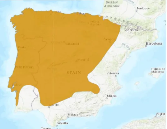
Figure 3.1- Hyla molleri distribution range and climate influence on the Iberian Peninsula. Map
adapted from the IUCN List of Threatened species………..…….7
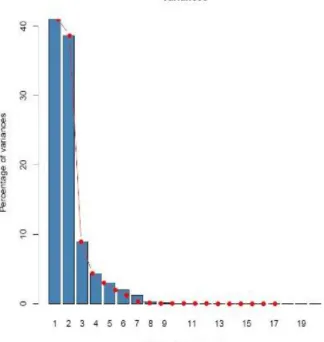
Figure 4.1- Percentage of variance explained by each PC………..13
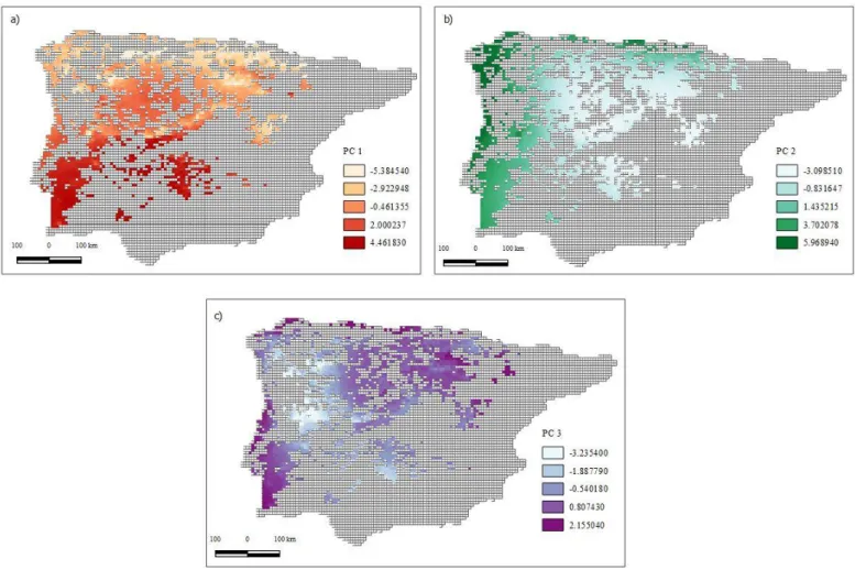
Figure 4.2 - First three PCs values across the species distribution. Values for PC 1 are represented in a); values for PC 2 are represented in b) and for PC 3 the values are represented in c). The colour gradient represents the range of values for each PC, being lighter colours lower values and darker colours higher values……….15
Figure 4.3 - Cluster Dendogram based on Mahalabonis distances showing relationships among climatic clusters………15
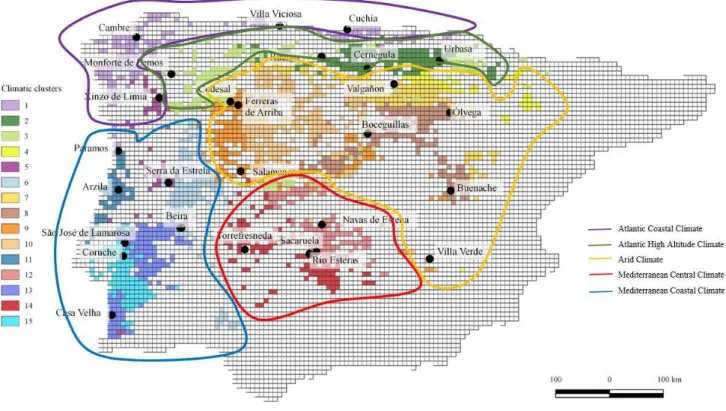
Figure 4.4 - Sampling locations within each of the climatic clusters………..………17
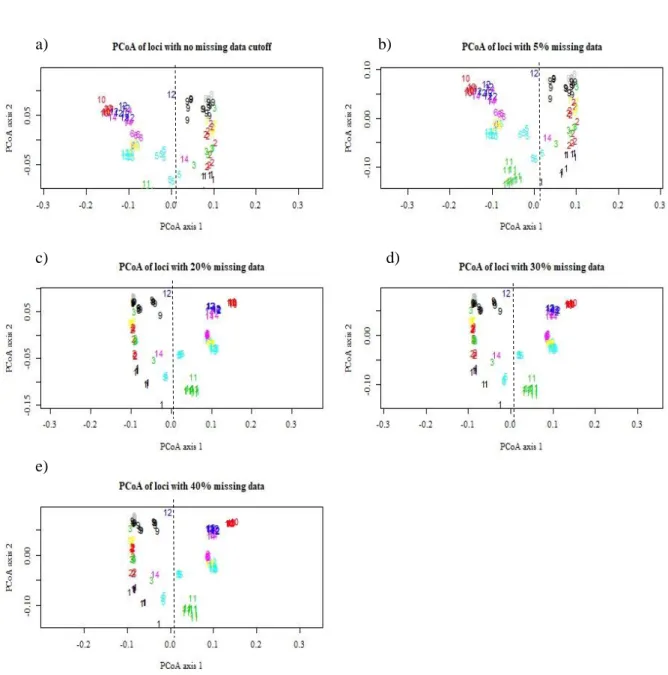
Figure 4.5 - PCoA results for the datasets with different cutoff levels of missing data at the locus and individual levels………..……….19
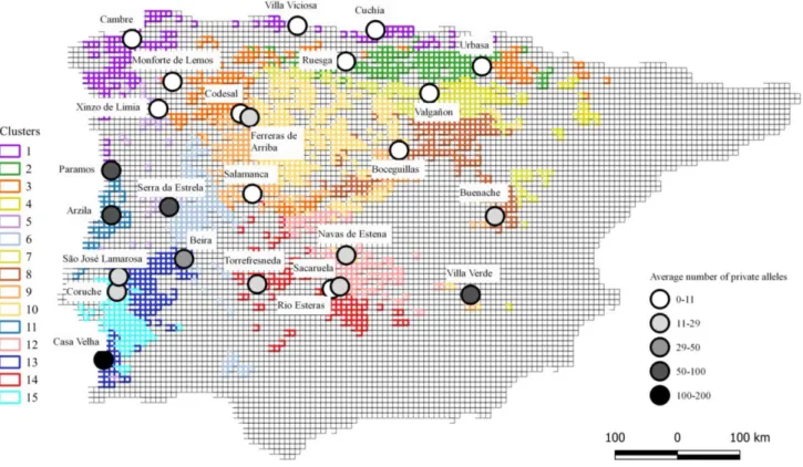
Figure 4.6 - Number of private alleles per location…………..………..……….20
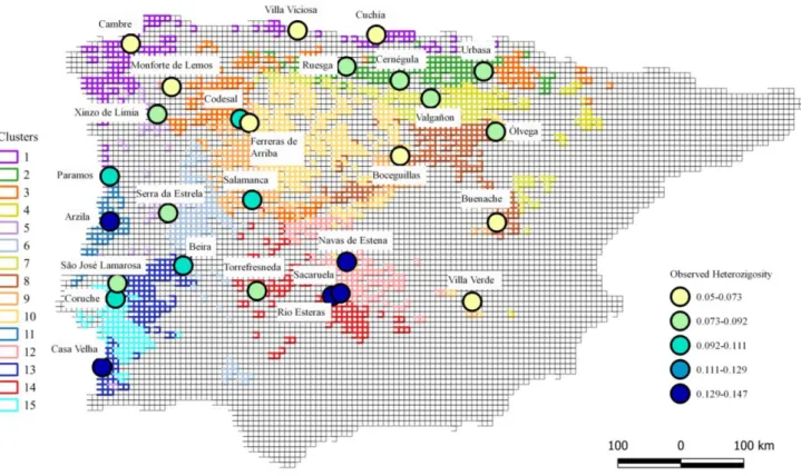
Figure 4.7 – Observed Heterozygosity for each population…..………..21
Figure 4.8 - z-scores for the power spectru….………...……….………21
Figure 4.9 - Global and local structures obtained by sPCA eigenvalues (left) and screeplot (right)………22
Figure 4.10- Two dimensional scatter plot of sPCA eigenvalue first (left) and second (right) axis………22
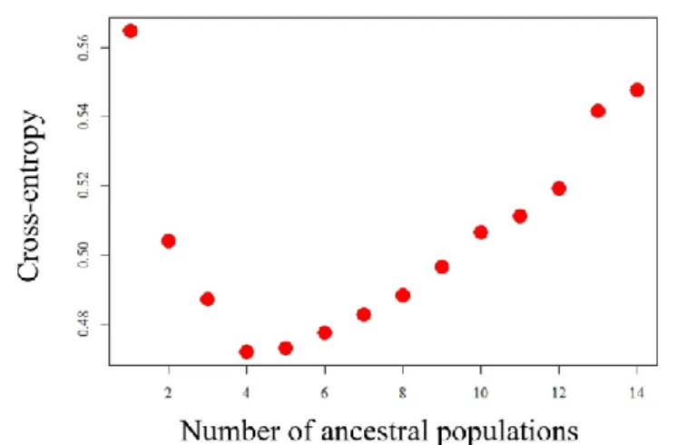
Figure 4.11 - Cross-entropy values for the run with the data set with 20% missing data for both for loci and genotypes………...………...22
Figure 4.12 - Bar plot of ancestry coefficients for each individual when K = 2. Each colour represents one ancestral group………..23
Figure 4.13 – Bar plot of ancestry coefficients for each individual when K= 4. Each colour represents one ancestral group………..24
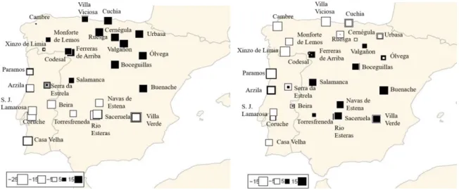
Figure 4.14.- Pie charts showing the average admixture coefficient of individuals per sampled locality for K = 2 (top) and K=4 (bottom). ……….………..…………...25
1
1.
INTRODUCTION
1.1 G
LOBAL AMPHIBIAN DECLINE
Global decline of amphibian population has become a major concern for the scientific and conservation communities1–4. Although the threats are known (e.g. habitat loss,
over-exploitation, agricultural expansion, invasive species, anthropogenic climate change, increased UV-radiation, road mortality and the harvest for human consumption5,6)the exact drivers of the
declines are not fully understood4. Additionally, the International Union for Conservation of
Nature (IUCN) Red List of Threatened Species shows that 41% of amphibian species are currently threatened with extinction. This places amphibians at a greater conservation concern compared to other vertebrates6.
The main environmental factor shaping amphibian distributions is water availability, as it impacts both phases of amphibian life cycle due to desiccation risk7. Eggs and larvae have a
mortality risk associated with the water depth of ponds (or other lentic water sources) not being enough to counterbalance water evaporation7. Additionally, reduced water availability also leads
to smaller pond sizes, which will have many indirect effects, such as reduced food supply, alterations in tadpole density and smaller size at metamorphosis7. Adult amphibians, although
not completely water dependent, can also be prone to desiccation if faced with conditions in which water loss through the respiratory system and skin is elevated7. A decrease in
environmental moisture can also lead to limited periods of activity, diminished mobility, less capability to evade predators and a decrease in food supply7. Therefore, environmental
conditions highly influence amphibian colonization capability by having a direct impact in amphibian distribution.
Possible shifts in local environment due to climate change can also alter the distribution and abundance of some amphibian species by turning previously unfit locations into habitable places and vice versa8. The causes of these behavioural and demographic modifications are a
result of direct (e.g. changes in phenology, alterations to movement and new physiological stress) and indirect effects (e.g. different predators, competitors, habitat modifications and changes in food supply), which highly influence population dynamics8.
In light of the various environmental alterations felt worldwide attributed to climate change, several studies have been focused on climate change predictions and the effects they would have on various taxa. For amphibians, studies indicate that climate changes might intensify population fragmentation, diminish distribution areas, increase extinction rates and cause multiple alterations in biotic interactions9,10. Therefore, there is a need to study amphibian
population distribution with more detail and understand what factors are limiting and driving it.
1.2. T
HE IMPORTANCE OF GENETIC DIVERSITY FOR AMPHIBIAN
CONSERVATION
Other threats which have been largely overlooked are genetic factors, including low genetic diversity, increased genetic drift and inbreeding6. Genetic diversity results from the diversity of
alleles and genotypes found in species and, according to the IUCN11, constitutes a level of
biodiversity in need of conservation actions. By being the foundation of evolutionary potential, genetic diversity is crucial for a species’ capacity to overcome changes in population fitness, acting as a safeguard in the event of unexpected and catastrophic events that can strongly
2 diminish population size6. Essentially, genetic diversity is what allows for the development of
adaptive responses that species need for their long term survival12.
Genetic diversity can be classified into two categories: adaptive or neutral13. The first is under
selection and has an effect on individual fitness; the second is not under selection and provides insights into population dynamics and evolutionary forces (i.e. genetic drift, mutation, migration)13. Conservation biologists have been focusing on neutral diversity13, mostly to define
Conservation Units (CUs) within species14, which are essential in the development and
management of conservation efforts. Conservation priority is usually given to CUs that have genetic and ecological uniqueness (Evolutionarily Significant Units) and which populations are more influenced by their own dynamics than by immigration (Management Units)14. However,
adaptive variants are also crucial for species’ survival15 as they improve the population fitness
for different environmental conditions16. In fact, adaptive differences in relation to climate
gradients have been found among populations of the same species17.
From a genetic point of view, amphibian populations are generally small, which translates into a small amount of active breeders6 and are more prone to have low genetic diversity due to
arbitrary genetic drift18. Additionally, their reproductive output, reproductive success and
mortality rates can vary greatly from one year to another due to their dependence on water availability6. This high sensitivity to external factors has lead Allentoft & O’Brien (2010) to
hypothesize that in the event of severe predatory pressure or extreme heat (leading to desiccation), it is possible that only a few egg clutches survive leading to a population entirely constituted by siblings6, thus showing how an amphibian population can be affected by
inbreeding in just one reproductive cycle. Thus, amphibian populations are likely to have higher levels of homozygosity and low genetic diversity enhancing the risk of inbreeding depression in populations, which can result in lowered fitness6, increasing extinction risk18.
Additionally, the impact that genetic diversity loss has in populations is a long term impact, meaning that reversing its effects is more difficult19. Therefore, maintaining genetic diversity
within species populations is vital for their survival.
Scientist tend to regard amphibian populations as metapopulations: during the reproductive season, most species of amphibians aggregate in ponds to mate and lay their eggs8, with ponds
differing greatly among each other (e.g. in diameter, depth, vegetation, coverage, etc.), granting each pond the status of a population8. In metapopulations, migrant exchange (i.e. gene flow) and
colonization dynamics (i.e. local extinctions and recolonizations) ensure a balance between events of colonization and extinction8. However, if amphibian metapopulations become isolated
(e.g. due to habitat fragmentation), gene flow will diminish and populations will be more affected by inbreeding, genetic drift and selection, therefore becoming more prone to loss of genetic diversity, reduced fitness, and higher extinction rate6. For instance, human-induced
habitat fragmentation in the Lolland island populations of H. arborea (Linnaeus, 1758) led to population bottlenecks, with most populations suffering severe genetic diversity loss7. Some
populations were even at risk of extinction due to high levels of inbreeding7.
Habitat characteristics, such as elevation or geographical distance, can also impact amphibian genetic diversity by acting as a barrier to dispersal given the energy required to move between places13,20. The combination of low dispersal ability and specific habitat needs (e.g. high
moisture levels) can also limit population connectivity and lead to high levels of genetic drift6.
Moreover, the species’ biogeographical history can also play a major role in genetic diversity21.
Garner et al. (2004) verified this in a study that revealed that Rana latastei (Boulenger, 1879) genetic diversity followed an east-west gradient, caused by several founder events during the
3 species expansion from the Balkan area, which served as a glacial refugium21. Hence,
understanding whether low genetic diversity is caused by human action, by biological features, biogeographic history or a combination of factors, is important from a conservation point of view since it will influence conservation actions6.
Spatial patterns of genetic diversity in amphibian taxa appear to be strongly influenced by historical processes and less so by current events18, 21, , with most taxa presenting multiple
geographically structured mitochondrial DNA lineages21.
1.3. T
HE IBERIAN PENINSULA AND AMPHIBIAN DISTRIBUTION
The Iberian Peninsula is considered a biodiversity hotspot, because it holds a high number of endemic species. In addition, many species present high intra-specific diversity, which is often spatially structured10. Several factors have contributed to turning the Iberian Peninsula in a
biodiversity hotspot, such as geological events (land connection with the African continent allowing for African species to colonize), geographical characteristics (large mountain ranges with an east-west orientation that allows for microclimates to develop, providing a refuge for populations when climate shifts, allowing for their survival18, 21), climatic influence (from
Atlantic to Mediterranean and Desert climate) and climatic history (e.g. Pleistocene Ice Ages)18,21. The latter played an important role in the number of endemism’s found in Iberia
since this area functioned as an important glacial refugia18.
In fact, the Pleistocene Ice Ages deeply altered Iberian species distribution through repeated local extinctions, dispersal to new locations, concentration in refugia and expansion from there, etc.18, resulting in strong genetic structure and divergence among populations21. This genetic
patterns across several species range point to several refugia within the Iberian Peninsula during the Pleistocene: a refugia-within-refugia hypothesis21. Suggested by Gómez & Lunt (2007), the
refugia-within-refugia hypothesis amounts to seven refugia within the Iberian Peninsula, being the majority found in the south. Gómez & Lunt (2007) also compiled data showing a higher genetic diversity in the south of the Peninsula since southern populations appear to be more demographically stable21. However, not all refugia appears to have been adequate throughout
the Ice Ages, meaning that the same species might have taken refuge in different refugia in different glaciations21.
Except a few exceptions, Iberian amphibians were also more likely to have taken refuge in the south, more specifically in the Betic Range and in Central Portugal (Serra da Estrela)21.
1.4. L
ANDSCAPE GENETICS
Landscape genetics encompass a sampling design focused in landscape characteristics and using a range of genetic and statistical tools to find patterns of genetic diversity that can be explained by one or several landscape/environmental characteristics22. Landscape can influence the
genetic patterns of a species mainly through two processes: by-distance and isolation-by-environment23. In isolation-by-distance it is the increasing geographical distance and barriers
that drive genetic differentiation due to reducing gene flow among populations20; in
isolation-by-environment it is the environmental differences that push adaptive genetic differentiation limiting gene flow by means of natural selection, independently of geographical distances23.
Landscape genetics tries to disentangle the effect of both of these processes to shed some light in the species’ genetic patterns.23
4 With such goals in view, the first step in landscape genetics is to identify genetic patterns across the landscape and the second step is to associate those patterns with landscape composition22. In
order to identify the genetic patterns, researchers must collect genetic data from as many individuals as possible and register the exact geographical location of the sampling22. Here, the
individual is the preferable study unit, as it provides more detailed result22. Nevertheless, if
enough populations are sampled, through the use of allele frequencies, each population can be the study unit22.
Since the main threats to the focus species of this thesis are landscape features (that can lead to isolation), it was important to incorporate this analysis in an attempt to better understand which drivers can be affecting H. molleri population structure and genetic diversity.
1.5. S
INGLE NUCLEOTIDE POLYMORPHISM (SNP’s)
In this work we focused on using SNPs and DArTseq technology to study H. molleri (Bedriaga, 1890) population structure and genetic diversity.
When a mutation affects a single nucleotide position at a locus, creating an allele with an alternative basis it originates a SNP – Single Nucleotide Polymorphism-24. Therefore, SNPs can
be considered as the final cause for genetic differences between individuals24.
Despite microsatellites and simple sequence repeats being the most used genetic markers in genetic diversity studies25, they are quickly being replaced by SNPs, for SNPs are more
abundant and stable26, amenable to automation, efficient and gradually more cost-effecient25.
Additionally, the development of restriction site-associated DNA sequencing (RADseq) methods27, has allowed for SNP development with simultaneous discovery and genotyping for
non-model species28. RADseq methods create DNA libraries and are a fast, robust and
cost-effective high-throughput method for genetic diversity and population structure analysis in non-model species28. Diversity Arrays Technology – DArT – is a RADseq method that first uses
restriction enzymes to reduce genome complexity and then employs hybridization to microarrays to discover several hundred polymorphic loci across the entire genome, without requiring a priori information of the genome29.This method actively selects portions of the
genome with active gene, which is an advantage when working with species with large genomes (such as amphibians). Additionally,by determination of the most fitting method for complexity reduction, this technology is enhanced for both the organism and application chosen, providing several thousand markers at a relatively low cost per sample30
1
.
6. H
YLA MOLLERI AS A CASE-STUDY SPECIES
Hyla molleri is an Iberian endemism, belonging to the Hylidae family whose origin and diversity is located in the neotropics31, 32. In fact, within the hylidae, only the genus Hyla
extends into the Palearctic region, including four species groups: arborea, cinerea, versicolor and eximia33, with the arborea group dispersing into Europe34.
In the Iberian Peninsula, two species of Hyla can be found: H. molleri and H. meridionalis (Boettger, 1874)33. Hyla molleri is mainly found in the North and Central part of the Iberian
Peninsula44 and H. meridionalis in the Mediterranean coastal zone and the South34, with the
central part of the Peninsula acting as a sympatry zone where hybridization can occur, originating unfertile hybrids34.
5 Hyla molleri was considered to be H. arborea or a subspecies of H. arborea (H.a.molleri) until recently31. The H.a.molleri designation was based in morphological criteria (such as body length
and the length of the posterior limbs) which did not provide enough scientific support to be accepted as a separate species by the scientific community34. In 2008, Stock et al. showed that
the Iberian population was distinct from the rest of the European populations31.
The Spanish populations of H. arborea were classified as “Almost Threatened”, prior to revision of its taxonomic status, due to population isolation in the eastern and south-western regions35. These populations may still be declining in the more arid regions due to loss
of sites suitable for reproduction35. In Portugal, H. molleri has also several populations that
appear to be isolated, such as those near the Douro and Minho rivers, Serra da Padrela and Alvão36. In addition, Rosa & Oliveira (1994) found H. molleri to have lower genetic diversity
than expected in a genus already shown to have low genetic diversity345.
The putative declining population sizes and increased isolation raise concerns regarding its long term survival and the need to critical evaluate the current conservation status.
Despite the above mentioned alarming signals of declining population sizes and connectivity, data regarding the species´ current population structure and levels of gene flow among populations are scarce.
Before the official separation from H. arborea, Rosa & Oliveira (1994) studied the genetic differentiation between H. meridionalis and “H. arborea molleri”, and found very low values of genetic diversity, even suggesting that the samples could be perceived as the result of a single population with random mating, regardless of their distance35.
Since the official separation of H. molleri from H. arborea, few studies have been conducted on the species’ population structure. The following studies are, to the extent of my knowledge, the ones that have done so:
Barth et. al (2011)38: In this study, researchers studied genetic diversity at mitochondrial
genes in populations across the Iberian Peninsula. The sampling efforts were focused in Galicia, due to the combination of Mediterranean climate in the southeast and Atlantic climate in the north. Here preliminary data had indicated weak genetic differentiation in populations located in the northern coast of Galicia. The results showed: i) low mitochondrial differentiation of populations across the Iberian Peninsula; ii) no significant correlation between genetic distance and geographical distance; iii) weak genetic differentiation between populations located in the coastal area of Galicia and populations in central Spain; and iv) possible areas of admixture in inland Galicia and in northwestern Spain and northern Portugal. In light of these results, the authors concluded that there seems to be a considerable amount of gene flow or recent population expansion in Iberia. However, due to the uneven geographical sampling (several populations and multiple specimens per population in Galicia and smaller sample sizes from central Spain), the results might have lead to erroneous interpretation of population differentiation and isolation by distance. Yet, it is important to acknowledge the research developed by Gvozdik et. al (2015)39, on speciation history and introgression of several European Hyla
species, where the authors also found a distinct haplotype in Galicia. This suggests that this region might have played a role as a glacial refugium.
Stock et. al (2012)33: Here the authors used mitochondrial and nuclear markers to define the
6 knowledge of anuran dispersal capability, they expected to find that altitude zones (e.g. mountains such as the Alps, Pyrenees and Carpathians), are important barriers to gene flow, keeping gene flow restricted to low altitude areas. They also expected to find varying amounts of geographic genetic structuring among H. molleri’s distribution range, with lower diversity in the northern regions and higher endemism in the southern ones (due to more stable climate during the last glaciation). The results showed: i) low genetic structure within species; ii) range overlap and hybridization of H. molleri and H. arborea in the southwest of France, and iii) little mtDNA diversity throughout the H. molleri range. However, this study had limited sampling for H. molleri (i.e. only 37 out of the 462 individuals sampled-, and only one locality was sampled in France versus two localities in northern Spain and the rest in central Spain. Therefore, this sampling may have biased the results, which may have led to unreliable conclusions.
Moreira, C. (2012)40: While studying from a molecular and bioacoustics approach the
populations of H. molleri and H. meridionalis in Portugal, this researcher found two divergent groups of mtDNA haplotypes in H. molleri, namely on group occurring in sites located south of the Mondego River and another group occurring in sites north of the Mondego River and northwest Spain. Additionally, within each group, high levels of haplotype diversity were detected, indicating a high level of genetic diversity, contrary to previous studies.
Sánchez-Montes et. al (2019)41: Through the use of mtDNA and microsatellites specific for
this species, the authors reconstructed the historical biogeography of H. molleri. Sampling included 248 individuals from 60 localities, covering the species whole distribution. Their results showed 1) higher genetic diversity in the northern Iberian mountains and western areas, 2) a concentration of private alleles in the extremes of this species distribution and 3) genetic structure was better explain when K=4 or K=7.
So, despite the important insights into H. molleri population structure these studies provided, with exception to Sánchez-Montes et. al (2019), none of these studies has comprehensively studied the genetic population structure of the species across its entire range, or has had a sampling design that allowed for more robust conclusions. Additionally, these studies have been using mtDNA, microsatellites or a combination of both as their chosen genetic marker.
Therefore, there is a need for further studies regarding this species’ spatial genetic diversity patterns.
Environmental and geographical distance influence on genetic distances is also unclear for amphibians. Species such as Alytes obstetricans have suggested that species-characteristic genetic diversity drivers are the main factor the spatial patterns observed and not the environment itself42. However, Reino et. al (2017)43found that this species was more prone to be
present in areas with time-concentrated precipitation. Therefore, research on environmental influence in H. molleri genetic distance is required. As for geographical distance influence in genetic distance, a positive correlation between geographical and genetic distances for H.
molleri has been found by Barth et. al (2011), and Reino et. al (2017) found that this species
was more abundant in areas with lower slope. This points to geographical distance as a possible barrier to dispersal, meaning that further analysis should be conducted on H. molleri.
2. O
BJECTIVES
7 1) Infer the spatial genetic population structure, across the whole range of H. molleri; 2) Analyse the influence of geographic and environmental distances on the distribution of
the genetic diversity of H. molleri.
These objectives will be accomplished by sampling tens of individuals across the species’ range and using of DArTseq technology for simultaneous calling and genotyping of several thousands of SNPs distributed across the genome
3. M
ETHODS
3.1 S
TUDY AREA
The study area included the whole distribution range of H. molleri in the Iberian Peninsula. The Iberian Peninsula is located in the southwest corner of Europe and it includes Portugal and Spain’s continental territories, as well as Andorra, Gibraltar and a small portion of French territory in the north-eastern part. It is mainly influenced by two types of climate: Mediterranean climate – the most influential climate due to the influence of the Mediterranean Sea, which is predominant in the southern part of the Peninsula-, and is characterized by very dry summers and high precipitation during the winter; and Atlantic climate –which predominates in the north and northwest of the Peninsula, as well as in the major mountain systems, which is characterized by having cool temperatures year round, with little oscillation in the annual temperature range. H. molleri distribution does not include the whole Iberian Peninsula as this species mainly occurs in the North, Center and Western part of the Peninsula34(Figure 3.1).
3.2
.
E
NVIRONMENTAL STRATIFICATION FOR TISSUE SAMPLING
Figure 3.1- Hyla molleri distribution range and climate influence on the Iberian Peninsula. Map adapted from the
8 Sampling sites for tissue collection were chosen in order to cover the whole species’ distribution range and the whole climatic variability throughout the species range. This strategy was selected to allow testing for the effect of environmental heterogeneity on the distribution of genetic diversity of H. molleri.
Species’ distribution records were obtained from the Portuguese and Spanish atlases of amphibians and reptiles35,36 and from the database of the Spanish Herpetological Society
(http://siare.herpetologica.es/). Both atlases are referenced to a 10x10 km resolution UTM grid. To ensure coverage of the whole climatic variability, the species’ range was assessed for its spatial heterogeneity in a set of climatic variables which were subjected to a Principal Component Analysis (PCA) to reduce data dimensionality, followed by a model-based clustering method to identify the most likely number of climatic clusters.
Twenty variables were retrieved from the WorldClim database44 covering the species’ range (at
2.5 minutes resolution). The variables included annual mean temperature, mean diurnal range, isothermality, temperature seasonality, maximum temperature of warmest month, minimum temperature of coldest month, temperature annual range, mean temperature of wettest quarter, mean temperature of driest quarter, mean temperature of warmest quarter, mean temperature of coldest quarter, annual precipitation, precipitation of wettest month, precipitation of driest month, precipitation seasonality, precipitation of wettest quarter, precipitation of driest quarter, precipitation of warmest quarter, precipitation of coldest quarter and altitude.
The first three principal components (PCs) were obtained from the PCA, using the princomp function in R, and used to estimate the most likely number of environmental clusters throughout the species’ distribution using model-based clustering implemented in the R package mclust45.
The mclust package uses an Expectation-Maximization (EM) algorithm (which finds the maximum likelihood parameters) to perform the clustering analysis, ensuring that each cluster includes locations with similar climatic conditions. We ran Mclust with G = 1:16, being G the number of clusters for which the Bayesian Information Criterion (BIC) is calculated. The BIC is an index used to compare two or more alternative models, by valuing model fitness and reduced model complexity. The model with the lowest BIC is considered the best45. For the clusters
identified in the best model, we analyzed similarity between clusters using the mahalanobis distance. This distance was calculated based on the first 3 PCs using the pairwise.mahalanobis function from the HDMD R package46. Mahalanobis distances were then used to perform a
hierarchical cluster analysis using the complete linkage method (function hclust in R).
In addition to this, we also identified the variables with highest loadings for each PC and created raster layers for each PC for spatial visualization of the corresponding patterns. We also analyzed each climatic variable value distribution for each climatic clusters using boxplots.
3.3. F
IELDWORK
Sampling included 2-3 different locations per environmental cluster and 4-5 individuals per location. This sampling design was meant to ensure representation in the final dataset, and guarantee sufficient genetic data per cluster. Tissue collection was carried in the late Spring/early Summer of 2017 and included tadpoles (i.e. tip of the tail) and adults (i.e. first phalange of one of the posterior members). We registered the corresponding GPS coordinates of each sampling site. Sampling gaps were filled with museum samples collected (between 2013 and 2015) by Iñigo Martinez-Solano).
9
3.4. M
OLECULAR DATA COLLECTION
3.4.1. DNA extraction
We conducted genomic DNA (gDNA) extractions at CIBIO-InBIO laboratory, using the ExtractMe Genomic DNA 96-Well kit (DNA GDAŃSK) and QIAamp DNA Micro Kit (QIAGEN GmbtH), depending on the amount of tissue sample available. We followed the manufacturer’s instructions in all extraction procedures. We used agarose gel electrophoresis (0.5% w/v) run at 300 V in 0.5X TAE buffer to assess the extracted gDNA quality and quantity, and used PicoGreenTM fluorometry in VICTORTM (Perkin Elmer) to determine its concentration.
3.4.2. SNP development in Hyla molleri
We calculated the quantity of gDNA needed from each extraction so that every sample had 500 ng of gDNA. The samples were evaporated and reconstructed with 10 μL of pure water so that every sample had equal concentration: 50 ng gDNA/ μL. This step maximizes the probability of equal representation of reads across samples, and thus of the number of SNPs called and genotyped per individual. The gDNA samples were sent to Diversity Arrays Technology Pty Ltd, where simultaneous SNP calling and genotyping was done using proprietary DArTseq technology (Diversity Arrays Technology)44.
3.5. R
AW DATA TREATMENT
DArTseq output presented genotypes coded with “0”, “1”, “2” or “-“, indicating whether the individual was a homozygote for the reference allele, a homozygote for the alternative allele, an heterozygote or whether the genotype was missing, respectively. To facilitate data analyses in the Rstudio environment46, we transformed the raw data matrix into a genind object (which
stores individual genotypes) using the function df2genind from the adegenet package, to allow computations using several packages, including adegenet48 and poppr49. For that purpose the raw matrix was transposed so that individuals were in rows and loci in columns, and replaced the genotype codes “0”, “1”, “2” and “-“ with “AA”, “TA” ,“TT” and “NA”, respectively. We performed a preliminary analysis to assess how many SNPs had a call rate higher than 0.8, i.e. with genotype informations found in at least 80% of sampled individuals, which corresponds to SNPs with less than 20% missing data.
We then performed a Principal Coordinate Analysis (PCoA) on the genotype matrix. The PCoA allows data exploring and visual representation based on genetic distances among data points50.
The individual genotypes were used to estimate the proportion of shared alleles (function propShared from adegenet package48), and this individual genetic distance was used to perform
the PCoAs as implemented in the dudi.pco function of ade4 package. We first used PCoA on the whole data set (no loci or individuals removed) to detect putative outlier individuals, and then on several datasets with different cut-offs for missing data at the locus- (i.e. loci missing genotypes at some samples) as well as at the individual-level (i.e. individuals missing genotypes at some loci), obtained through the missingno function (poppr package).
Upon removal of putative outlier individuals, loci identified as monomorphic were removed.
3.6. G
ENETIC DIVERSITY
10 In order to understand how genetic diversity is distributed in H. molleri we calculated two different genetic diversity indices: average number of private alleles per locality and observed heterozygosity. These metrics allowed having different perspectives on genetic diversity and hence, have a better understanding of genetic similarities and differences among sample localities.
Private alleles are unique alleles found in each population, which provides a good, yet easily interpretable, measure of genetic differentiation among populations51. If gene flow is high
among populations, the fixation of distinct alleles is difficult, meaning this population will show lower values of private alleles51. To calculate the number of private alleles, we used the
private_alleles function (poppr package49).To avoid biased results due to differences in the
number of individuals sampled in each locality, we divided the number of private alleles per locality by the number of sampled individuals in each locality.
We calculated the observed heterozygosity for each locality of the whole dataset, using the summary function of the genind object as implemented in adegenet.
3.7. D
ETECTION OF PUTATIVE NON-NEUTRAL LOCI
In order to assess the distribution of neutral vs. adaptive diversity in H. molleri, we used the Moran Eigenvector Maps (MEM) approach described in Wagner et. al (2017) to detect putative outlier loci52. This approach relies on the assumption that adaptive loci behave as outliers, by
showing a distinct spatial signature compared to neutral loci, due to the result of selection rather than of gene flow52.
First, we used a Gabriel Graph to obtain a neighbour network and obtained a spatial weights matrix, which is needed to calculate the MEM axes. In the next step we obtained the power spectrum for each locus by calculating the squared of the correlations of each MEM axis with a matrix of allelic frequencies. The power spectrum shows the amount of variance that each locus has linked with each MEM. The average power spectrum across loci is then subtracted from each locus to obtain the standardized z-scores (i.e. standard deviation from the mean of each locus). We then used three cutoff values to identify outliers: 0.05, 0.01 and 0.001.
3.8. P
OPULATION STRUCTURE ANALYSIS
3.8.1. Spatial Analysis of Principal Components (sPCA)
We conducted a sPCA to identify the spatial genetic pattern within our sampling area and provide further insights about the species’ genetic population structure50.
The sPCA aims at finding independent synthetic variables (the principal components) which optimize the product of genetic variance and spatial autocorrelation of the haplotype frequencies of multiple loci. The spatial autocorrelation is measured using the Moran’s I statistic based on the samples’ geographical position and their allelic frequencies50. When allelic frequencies at
neighboring sites are more similar than expected at random, there is positive spatial autocorrelation (i.e. global structure)50. If allelic frequencies are more genetically distinct than
randomly expected, the spatial autocorrelation is negative (i.e. local structure) 50. Since the
variance of allelic frequencies term is always positive, the signal (positive or negative) of the obtained sPCA eigenvalues define if the spatial autocorrelation is positive (global structures) or negative (local structures).
11 We used the spca function implemented in the adegenet package with the Delaunay’s triangulation as the connection network to establish neighboring sites, since this method requires that if a circle is drawn through three nodes it ensures that any point on the surface is as close as possible to a node.
We performed Monte Carlo simulations to statistically test the significance of observed global and local structures (global.rtest and local.rtest functions), using 999 permutations.
We evaluated which eigenvalues should be further analysed - based on whether they contained enough variability and spatial structure - through the screeplot function, in which the eigenvalues of the sPCA (λᵪ) are represented according to their variance and Moran’s I value. Only the eigenvalues that show the highest variance and spatial autocorrelation should be used50. We then plotted a two dimensional scatter plot based on each individual score on the
selected eigenvalues, onto an Iberian Peninsula map (s.value function from the adegraphics package), to visualize the genetic differences/similarities amongst individuals.
3.8.2. Sparse Non-Negative Matrix Factorization (snmf) analysis
In order to gain further insights into H. molleri current population structure, we used a snmf analysis which provides an independent perspective of genetic differentiation and allows comparing results among analytical approaches.
We used the snmf function of the LEA package54, that uses sparse Non-Negative Matrix
Factorization algorithms, to estimate individual ancestry coefficients and ancestral allele frequencies54. Sparse Non-Negative Matrix Factorization is an unsupervised statistical method,
meaning that it uses likelihood methods to infer ancestral gene pools instead of predefined populations55. This algorithms reduces data dimensionality and allows for hidden data structure
to become known54.
We chose this approach in place of other more often used methods, such as STRUCTURE software55-59, because snmf is faster55, allows for more efficient data exploring, is more suitable
for large datasets with many loci, and the choice of number of genetic clusters is based on a cross-validation criterion, which may be more reliable than those used in other methods53. In
addition, the output has a very easy interpretation as the percentage of each ancestry lineage found in each individual can be displayed using a barplot.
To use this function we had to create a geno object. The geno object is a file format that stores the data with one row for each SNP53 For the number of ancestral populations for which the
snmf algorithm estimates have to be calculated (K)53, we choose from 1 to 14, given that there
were 14 environmental clusters and the sampling strategy aimed at collecting individuals on a per-cluster basis. We ran the snmf function with 10 repetitions for each value of K with 1 000 iterations and for 3 alpha values (being alpha the regularization parameter, whose value can alter the results): 10, 100 and 500, to assess congruence of results. We then calculated the corresponding cross-entropy criterion for each run. This criterion assesses the fit of a model with K populations: a smaller value of cross-entropy equals a better prediction capability for that run53.
We used the most likely K value, i.e. with lower cross-entropy values, in the cross.entropy function to create a Q-matrix (i.e. individual admixture coefficient matrix) and the resulting barplots. For easier visualization of the spatial distribution of individual genetic admixtures, we used QGIS software (2.14.20 version) to plot individual pie charts on a map.
12
3.9
.
L
ANDSCAPE GENETICS
For the landscape genetics analysis we tested IBD and IBE simultaneously by performing a multiple matrix regression with randomization (MMRR) analysis on matrices of genetic (response variable), geographical and environmental distances (explanatory variables)61. This
analysis allowed us to test if spatial distances and environmental heterogeneity had an effect on the genetic distribution of H. molleri. The MMRR output is a multiple regression equation, that tests if the dependent variable changes with respect to the different independent variables61, and
if so, how is that change. Thus, the regression coefficients quantify how the genetic distances respond to variation in environmental and geographical distances; the coefficient of determination evaluates the overall fit of the model (R2) and the p-value allows to infer statistical significance of the coefficients61.
Since this analysis runs at the population level, we used pairwise FST as the genetic distance. As
for the environmental distance, since the sampling approach adopted for this study aimed to include individuals from the 14 environmental clusters defined using a PCA (see above for details), the loadings of the first 3 PCs of each locality were used to estimate multivaried euclidean environmental distance among pairs of localities. Finally, the geographical euclidean distances (in kilometres) were calculated using the GeoDistanceInMetresMatrix function, which uses geographical coordinates to calculate the euclidean distance between two points.
Because FST was used as the genetic distance, only populations with more than one individual
were used in this analysis. The pairwise FST values were estimated using the pairwise.fst
function implemented in the hierfstat package62.
Prior to implementing the MMRR we assessed the data for linearity by fitting linear models of the genetic distance (dependent variable) in function of the geographical distance (independent variable). We also scaled and centered the geographical distance matrix, to reduce bias introduced by different absolute values among distance matrices.
The MMRR was performed with the lgrMMRR function as implemented in the PopGenReport package63, with 999 permutations to assess statistical significance.
13
4. R
ESULTS
4.1. E
NVIRONMENTAL STRATIFICATION FOR SAMPLE COLLECTION
The first three PCs explained 88.6% of the variance in the climatic data set (Figure 4.1).
Table 4.1 - List of the most important climatic variables for each of the first three PCs. Loadings of each variable in
parentheses.
PC Most important variables
PC 1
Mean Temperature of Warmest Quarter (0.33) Precipitation of Driest Quarter (-0.32)
Precipitation of Warmest Quarter (-0.32) Max Temperature of Warmest Month (0.31)
PC 2
Temperature Annual Range (-0.32) Temperature Seasonality (-0.32) Precipitation of Coldest Quarter (0.31) Mean Diurnal Range (-0.31)
PC 3
Mean Temperature of Wettest Quarter (0.47) Isothermality (0.38)
Precipitation of Coldest Quarter (-0.32)
The loadings show how each variable contributes and behaves in each PC: when the variable signal is positive it means that when PC values increase so do the values of the variable; if the signal is negative it means that the variable value decreases as PC value increase. Taking that into account, PC 1 will have higher values where the mean temperature of the warmest quarter and the maximum temperature of the warmest month are higher and where the precipitation of the driest quarter and of the warmest quarter are lower, thus characterizing a warmer and drier
14 climate, as it is expected in areas with the Mediterranean climate. When observing the spatial distribution of the loadings (Figure 4.2a), PC 1 shows a north-south gradient, thus separating the two most felt climates in the Iberian Peninsula: the Atlantic climate, in the north, and the Mediterranean climate, in the south.
As for PC 2, the loadings indicate that this PC will have higher values where temperature annual range, temperature seasonality and mean diurnal range are lower and precipitation of coldest quarter is higher. This characterizes a climate with few fluctuations in temperature range and high precipitation during the winter. Figure 4.2b, shows that this PC has higher values in the coastal areas of the species range, indicating a separation between inland and coastal climates. Finally, for PC 3, the loadings display higher positive values for the mean temperature of the wettest quarter and isothermality and a negative value for the precipitation of the coldest quarter. This implies higher values for areas where temperatures are more constant, the rainy season has higher temperature and winters are drier. Figure 4.2c shows that PC 3 displays a periphery-center gradient with higher values in the periphery of the species range.
15
Figure 4.3 - Cluster Dendogram based on Mahalabonis distances showing relationships among climatic clusters Figure 4.2 - First three PCs values across the species distribution. Values for PC 1 are represented in a); values for
PC 2 are represented in b) and for PC 3 the values are represented in c). The colour gradient represents the range of values for each PC, being lighter colours lower values and darker colours higher values.
Legend
AC= Arid Climate
ACC = Atlantic Coastal Climate AHAC = Atlantic High Altitude Climate
MCoC = Mediterranean Coastal Climate
MCeC = Mediterranean Central Climate