A Study of Single- and Double-Averaged Second-Order Models to Evaluate Third-Body Perturbation Considering Elliptic Orbits for the Perturbing Body

(1)

Volume 2013, Article ID 260830,11pages http://dx.doi.org/10.1155/2013/260830

Research Article

A Study of Single- and Double-Averaged Second-Order

Models to Evaluate Third-Body Perturbation Considering

Elliptic Orbits for the Perturbing Body

R. C. Domingos,

1

A. F. Bertachini de Almeida Prado,

1

and R. Vilhena de Moraes

2

1_{Instituto Nacional de Pesquisas Espaciais (INPE), 12227-010 S˜ao Jos´e dos Campos, SP, Brazil}

2_{Universidade Federal de São Paulo (UNIFESP), 12231-280 São José dos Campos, SP, Brazil}

Correspondence should be addressed to A. F. Bertachini de Almeida Prado; bertachiniprado@bol.com.br

Received 6 November 2012; Accepted 29 April 2013

Academic Editor: Maria Zanardi

Copyright © 2013 R. C. Domingos et al. his is an open access article distributed under the Creative Commons Attribution License, which permits unrestricted use, distribution, and reproduction in any medium, provided the original work is properly cited.

he equations for the variations of the Keplerian elements of the orbit of a spacecrat perturbed by a third body are developed using a single average over the motion of the spacecrat, considering an elliptic orbit for the disturbing body. A comparison is made between this approach and the more used double averaged technique, as well as with the full elliptic restricted three-body problem. he disturbing function is expanded in Legendre polynomials up to the second order in both cases. he equations of motion are obtained from the planetary equations, and several numerical simulations are made to show the evolution of the orbit of the spacecrat. Some characteristics known from the circular perturbing body are studied: circular, elliptic equatorial, and frozen orbits. Diferent initial eccentricities for the perturbed body are considered, since the efect of this variable is one of the goals of the present study. he results show the impact of this parameter as well as the diferences between both models compared to the full elliptic restricted three-body problem. Regions below, near, and above the critical angle of the third-body perturbation are considered, as well as diferent altitudes for the orbit of the spacecrat.

1. Introduction

Most of the papers on this topic consider the third-body per-turbation due to the Sun and due to the Moon in a satellite around the Earth. his is the most immediate application of the third-body perturbation. One of the irst studies was made by Kozai [1] that developed the most important long-period and secular terms of the perturbing potential of the lunisolar perturbations, written as a function of the orbital elements of the Sun, the Moon, and the satellite. Moe [2], Musen [3], and Cook [4] studied long-period efects of the Sun and the Moon on artiicial satellites of the Earth. hey applied Lagrange’s planetary equations to study the variation of the orbital elements of the satellite and its rate of variation. his idea was expanded by Musen et al. [5] that included the parallactic term in the perturbing potential. Kozai [6] studied the secular perturbations in asteroids that are in orbits with high inclination and eccentricity, assuming that the bodies are perturbed by Jupiter. Blitzer [7] made estimates for the

lunisolar perturbation for the secular terms. Around the same time, Kaula [8] obtained the disturbing function considering the perturbations of the Sun and the Moon.

Later, Giacaglia [9] calculated the disturbing function due to the Moon using equatorial elements for the satellite and ecliptic elements for the Moon. All terms were expressed in closed forms. Kozai [10] worked again on that problem and expressed the perturbing function as a function of the polar geocentric coordinates of the Moon, the Sun, and the orbital elements of the satellite. he short-period terms are shown in an analytical form, and the secular and long-period terms are obtained by numerical integration.

(2)

the same technique for the prediction of orbits for a long time span.

In the last years, several researches, based on both ana-lytical and numerical approaches, studied the third-body perturbation. he majority of them concentrated on studying the efects of a perturbation caused by a third body using a double-averaged technique, like those of ˇSidlichovsky´y [14], Kwok [15, 16], Broucke [17], and Prado [18]. he disturbing function is expanded in Legendre’s polynomials, and the average is made over the periods of the perturbing and the perturbed body, using an approximated model expanded to some order. Some others studied this problem based on a single-averaged analytical model, where the disturbing func-tion is expanded in Legendre’s polynomials but the average is made over the short period of the perturbed body only; see, for example, [19] and references therein. In all of the researches cited before, the perturbing body was in a circular orbit. here are also several papers considering the third-body perturbation in constellations of satellites (see [20,21]) and in other planetary systems not involving the Earth, like those of Carvalho (see [22–25]), Folta and Quinn [26], Kinochita and Nakai [27], Lara [28], Paskowitz and Scheers (see [29,30]), Russel and Brinckerhof [31], and Scheers et al. [32]. In particular, Roscoe et al. [33] used the analytical equations derived in Prado [20] to study the dynamics of a constellation of satellites perturbed by a third body.

Using the double-averaged analytical model in Domingos et al. [34], the analytical expansion to study the third-body perturbation was extended to the case where the perturbing body is in an elliptical orbit. Liu et al. [35] included the incli-nation of the perturbing body’s equatorial plane with respect to its orbital plane.

he main idea behind the single-averaged technique is that it eliminates only the terms due to the short-time peri-odic motion of the perturbed body. he results are expected to show smooth curves for the evolution of the mean orbital elements for a long-time period when compared with the full restricted three-body problem. In other words, a better understanding of the physical phenomenon can be obtained, and it allows the study of long-term stability of the orbits in the presence of disturbances that cause slow changes in the orbital elements.

So, an interesting point would be a study to show the diferences between those two averaged models when com-pared with the full elliptic restricted three-body problem. he idea of the present paper is to study this problem, but assuming that the perturbing body is in an elliptical orbit. Studies under this assumption are available in Domingos et al. (see [34,36,37]). In particular, in the present paper, a study of the efects of the eccentricity of the perturbing body in the orbit of the perturbed body is made for several diferent conditions regarding the orbit of the primaries as well as the orbit of the spacecrat.

So, our goal is to make a more complete study of this problem and to perform some tests to verify the diferences in the results obtained by those two approximated techniques. A comparative investigation is made to verify the diferences between the single-averaged analytical model with the model

based on the double-averaged technique, as well as a compar-ison with the full restricted elliptic three-body problem that can provide some insights about their applications in celestial mechanics.

he assumptions used to develop the single-averaged analytical model are the same ones of the restricted elliptic three-body problem (planet-satellite-spacecrat). Our anal-ysis for the evolution of the mean orbital elements will be based only on gravitational forces. he equations of motion are obtained from Lagrange’s planetary equations, and then we numerically integrated those equations. Diferent initial eccentricities for the perturbing body are considered.

he set of results obtained in this research performs an analysis of several well-known characteristics of the third-body perturbation, like (i) the stability of near-circular orbits, to investigate under which conditions this orbit remains near circular; (ii) the behavior of elliptic equatorial orbits; and (iii) the existence of frozen orbits, which are orbits that keep the eccentricity, inclination, and argument of periapsis constants. A detailed study considering the “critical angle” of the third-body perturbation, which is an inclination that makes a near circular orbit that has an inclination below this value to remain near-circular, is made. his work is structured as follows. In Section 2, we present the equations of motion used for the numerical simulations.Section 3is devoted to the analysis of the numerical results for near circular orbits. he theory developed here is used to study the behavior of a spacecrat around the Earth, where the Moon is the disturbing body. he choice of the Moon as the disturbing body is made based on the fact that its efect on the spacecrat is larger than the efect of the Sun. Several plots show the time histories of the Keplerian elements of the orbits involved. Our conclusions are presented inSection 4.

2. Dynamical Model

For the determination of the equations of motion, we started by assuming the existence of a central body, with mass�₀, that is ixed in the center of the reference system�-�-�. he perturbing body, with mass��, is in an elliptic orbit with semimajor axis ��, eccentricity ��, inclination ��, argument of periapsis ��, longitude of the ascending node Ω�, and mean motion��. he spacecrat with negligible mass�is in a generic orbit with orbital elements:�(semimajor axis),� (eccentricity),� (inclination),�(argument of periapsis), Ω (longitude of the ascending node), and it has mean motion

�. his system is shown inFigure 1.

Using the traditional expansion in Legendre’s polynomi-als (assuming that�� ≫ �), the second-order term of the disturbing potential averaged over the eccentric anomaly of the spacecrat is given by the following (see [17,18,34]):

⟨�2⟩ = � �_�2_��2

2 (�

�

��) 3

{(1 + 32�2) [32 (�2+ �2) − 1] +154 (�2− �2) �2} ,

(3)

Z

Y

X

m0

m

r

r� m�

Figure 1: Illustration of the dynamical system.

where (Murray and Dermott [38])

��= �

�_{(1 − �}�2₎

1 + ��_cos_��,

cos��=cos��+ ��(cos2��− 1)

+ 98��2₍_cos_3��₋_cos_��_{) + ⋅ ⋅ ⋅ ,}

sin��=sin��+ ��sin2��

+ ��2

(98sin3��− 78sin��) + ⋅ ⋅ ⋅ . (2)

For the case of elliptic orbits of the perturbing body, the parameters�and �are written as follows (see [34]):

� =cos�cos� −cos�sin�sin�,

� = −sin�cos� −cos�cos�sin�, (3)

where� = Ω − ��− ��.

he mean anomaly��of the perturbing body is given as

��_{= �}�

�+ ��. (4)

hus, the variations in the orbital elements of the per-turbed body are obtained. To do this, we derived Lagrange’s planetary equations that describe the variations of the mean orbital elements of the spacecrat. he semimajor axis is constant, since the mean anomaly�was eliminated from the perturbing function. hose equations can be written as shown below:

��

�� = �154 ��2�√1 − �

2

�

× [sin2� (cos2� −cos2�sin2�)

−cos�cos2�sin2�] ,

��

�� = �sin�[�� (1 − �1 2)]1/2

3 4��2�2

× {�2[ − 5cos2�sin2�cos2�

+ 32 (−sin2� +sin2�cos2�)

−52sin�cos2� (1 +cos2�)]

+ (sin� −sin2�cos2�)

−5cos2�sin2�cos�} ,

�Ω

�� = �34��2 �

2

sin�[�� (1 − �2)]1/2

× {(1 + 32�2_{) (−}_sin2_�_sin_2�)

+ [cos2�cos2�sin2�

+sin�sin2�sin2�] (52�2)} ,

��

�� = �34��2{− �

2

sin�[�� (1 − �2)]1/2

× [(1 + 32�2) (−sin2�sin2�)

+ (52�2_{) (}_cos_2�_sin2_�_cos_2�)

+12sin2�sin2�sin2�] +√1 − �2

� × [5 (cos2� −cos2�sin2�)cos2�

− 5cos�sin2�sin2�

+62 (cos2� +cos2�sin2�)] } , (5)

where

� = 1 + 3��cos��+ 3��2cos2��

1 − 6��_{+ 15�}�2 . (6)

hose equations show some characteristics of this system compared with similar researches (see [18, 34]) which are listed as follows.

(4)

derivative of the inclination is not zero, so the orbit does not stay planar.

(ii) Elliptic equatorial orbits are not stable. he equatorial case (� = 0) has a singularity in the equation for the time derivative of the inclination, so this model is not able to make prediction for the behavior of the inclination. Regarding the eccentricity, it is visible that this case has a nonzero value for the time derivative of the eccentricity, so those orbits do not keep the eccentricity constant. he only exception is when the initial orbit is circular, as shown above, where the eccentricity remains zero. In fact, the equation for the time derivative of the eccentricity for equatorial orbits can be simpliied to the following:

��

�� = −�154 ��2�√1 − �

2

� sin2 (� − �) . (7)

(iii) hose facts explained above also show that there are no frozen orbits under this analytical model, which would be orbits where the time derivatives of the incli-nation, eccentricity, and argument of periapsis are all zero.

Domingos et al. (see [34]) made a similar study, but using the double-averaged technique and showed that circular and equatorial orbits exist in the double-averaged model, since orbits with zero initial inclination or zero initial eccentricity remain with zero eccentricity and zero inclination. he difer-ence in the equations of motion when considering the circular and the elliptic motion of the primaries under the double-averaged models is the existence of the term(1 + (3/2)��2+

(15/8)��4₎_{, which is an extra term that depends on the}

eccentricity of the primaries��and this term does not destroy those properties. he same is true for the frozen orbits, since the appearance of a multiplicative nonzero constant does not change this property.

3. Numerical Results

In this section, we show the efects of the nonzero eccen-tricities of the perturbing body in the orbit of the perturbed body. We numerically investigate the evolutions of the eccen-tricity and the inclination for a spacecrat within the elliptic restricted three-body problem Earth-Moon-spacecrat, as well as using the single- and the double-averaged models up to the second order. he spacecrat is in an elliptic three-dimensional orbit around the Earth, and its motion is perturbed by the Moon. To justify our study and to make it a representative sample of the range of possibilities, we used three values for the semimajor axis of the spacecrat: 8000 km, 26000 km, and 42000 km. hey represent a

Low-Altitude Earth Orbit, aMedium-Altitude Earth Orbit(the one

used by the GPS satellites), and aHigh-Altitude Earth Orbit

(the one used by geosynchronous satellites), respectively. he spacecrat is assumed to be in an orbit with the following initial Keplerian elements:�₀= 0.01,�₀= Ω₀= 0.

We focus our attention On the stability of near-circular orbits. Results of numerical integrations showed that this

stability depends on�₀ (the initial inclination between the perturbed and perturbing bodies). When �₀ is above the critical value (�_�), the orbit becomes very elliptic. If�₀ < �_�, then the orbit remains near circular (see [17, 18, 34]). he value of�_�is 0.684719203 radians or 39.23152048 degrees.

hus, for our numerical integrations, the initial inclina-tions for the orbit of the spacecrat received values near the critical inclination (in the interval�₀= 38∘and 41∘), below this critical value (�₀= 30∘, 20∘, 10∘, and zero), and then above this critical value (�₀=40∘, 50�, 60∘, 70∘, and 80∘). he eccentricity of the perturbing body is assumed to be in the range0 ≤

�� _{≤ 0.5}_{, in general, but some results are omitted when the}

approximations are found to be very poor. It means that we generalized the Earth-Moon system in order to measure the efects of the eccentricity of the orbit of the primaries.

All of the cases considering theLow-Altitude Earth Orbit

were simulated for 80000 canonical units of time, which correspond to 12800 orbits of the disturbing body. his time shows the characteristics of the system, since the third-body perturbations are weaker at�₀ = 8000km. he simulations for the other values of the semimajor axis were made only for 20000 canonical units of time, which correspond to 3200 orbits of the disturbing body, because it appeared to be a good number to evidence the characteristics of the system.

Our numerical results are summarized in Figures 2–6. Such igures refer to the orbital evolution of the eccentricity and inclination as a function of time for the initial inclinations cited above and a direct comparison between the models.

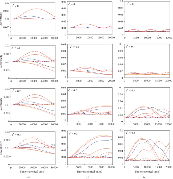
3.1. Low-Inclination Orbits. Figure 2shows the results of the evolution of the eccentricity as a function of time for the case where the initial inclination assumes the values�₀= 30∘(red line), 20∘(blue line), 10∘ (pink line), and zero (orange line). he irst, second, and third columns show the results for the cases ofLow-,Medium-, andHigh-altitude orbits, respectively.

Figure 2uses a solid line to represent the full elliptic restricted three-body problem, a dashed line to represent the single-averaged model, and a dashed-dotted line to represent the double-averaged model. Regarding the overall behavior, the results are according to the expected from the literature (see [17, 18]), and the increase of the initial inclination causes oscillations with larger amplitudes in the eccentricity. It is also clear that the averaged models are very accurate for the case where the perturbing body is in a circular orbit. his accuracy decreases with the increase of the eccentricity of the primaries for all values of the initial inclinations.

he use of second-order averaged models is not recom-mended for eccentricities of the primaries of 0.3 or larger. A larger expansion is required in this situation. In general, both averaged models have results that are much closer to each other than closer to those of the full model. It means that both averages tend to give the same errors, at least for eccentricities of the primaries up to 0.2. For eccentricity of 0.3 and above, the averaged models begin to show diferent behaviors, and those diferences increase with this eccentricity. Regarding the comparison between both averaged models, the results depend on the value of the initial inclination.

(5)

0 0.005 0.01 0.015 0.02

Eccen

tr

ici

ty

0 0.005 0.01 0.015 0.02

Eccen

tr

ici

ty

0 0.005 0.01 0.015 0.02

Eccen

tr

ici

ty

0 20000 40000 60000 80000 0 20000 40000 60000 80000 0 20000 40000 60000 80000 0 20000 40000 60000 80000

0 0.005 0.01 0.015 0.02

Eccen

tr

ici

ty

e�= 0.2

e�= 0.3 e�= 0

e�= 0.1

Time (canonical units)

(a)

0 0.01 0.02 0.03 0.04 0.05

0 5000 10000 15000 20000

0 0.01 0.02 0.03 0.04 0.05

e�= 0.2

e�= 0.3

e�= 0

e�= 0.1

(b)

0 5000 10000 15000 20000

0 0.02 0.04 0.06 0.08 0.1

0 5000 10000 15000 20000

0 0.02 0.04 0.06 0.08 0.1

0 5000 10000 15000 20000

0 0.02 0.04 0.06 0.08 0.1

0 5000 10000 15000 20000

0 0.02 0.04 0.06 0.08 0.1

e�= 0.2

e�= 0.3 e�= 0

e�= 0.1

(c)

Figure 2: hese igures show the evolution of the eccentricity as a function of time for low-inclination orbits. On the top of each igure is

shown the corresponding eccentricity of the perturbing body (��). In the irst column, the results are for the case ofLow-altitude orbits. he

second column is for the case ofMedium-altitude orbits. he third column is for the case ofHigh-altitude orbits. he lines are as follows: full

elliptic restricted three-body problem (solid line) and single-averaged (dashed line) and double-averaged models (dashed-dotted line). For

the colors,�0= 30∘(red line), 20∘(blue line), 10∘(pink line), and zero (orange line). he increase of the semimajor axis and the eccentricity

of the primaries reduce the average distance from the spacecrat to the Moon, making the perturbations stronger.

third-body perturbations are stronger. his fact accelerates the dynamics of the system, and the period of the oscillation of the eccentricity is shorter when compared with the low-altitude orbits. It is visible that high-low-altitude orbits have oscillations of eccentricity increased in amplitude with the

(6)

0.66 0.68 0.7 0.72 In clina tio n (rad) 0.64 0.66 0.68 0.7 0.72 In clina tio n (rad)

0

20000 40000 60000

0

20000 40000 60000

0

20000 40000 60000

0.64 0.66 0.68 0.7 0.72 In clina tio n (rad) 40∘ 41∘ 38∘ 39∘

e�= 0

40∘

41∘

38∘ 39∘

e�= 0.1

40∘

41∘

38∘ 39∘

e�= 0.2

Full Single 80000 80000 80000 Double (a) 0.66 0.67 0.68 0.69 0.7 0.71 0.72 0.66 0.67 0.68 0.69 0.7 0.71 0.72 0.66 0.67 0.68 0.69 0.7 0.71 0.72 0

5000 ₁₀₀₀₀ ₁₅₀₀₀

40∘

41∘

38∘

39∘

e�= 0

40∘

41∘

38∘

39∘

e�= 0.1

40∘

41∘

38∘

39∘

e�= 0.2

Full Single

0

5000 ₁₀₀₀₀ ₁₅₀₀₀

0

5000 ₁₀₀₀₀ ₁₅₀₀₀ ₂₀₀₀₀

20000

Double

(b)

0

5000 ₁₀₀₀₀ ₁₅₀₀₀

0.66 0.68 0.7 0.72 0.66 0.68 0.7 0.72 0.64 0.66 0.68 0.7 0.72 40∘ 41∘ 38∘ 39∘

e�= 0

40∘

41∘

38∘ 39∘

e�= 0.1

40∘

41∘

38∘ 39∘

e�= 0.2

Full Single

0

5000 ₁₀₀₀₀ ₁₅₀₀₀

0

5000 ₁₀₀₀₀ ₁₅₀₀₀

20000

Double

(c)

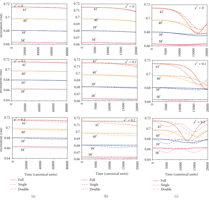
Figure 3: hese igures show the evolution of the inclination as a function of time for near critical inclinations. On the top of each igure is

shown the corresponding eccentricity of the perturbing body (��). In the irst column, the results are for the case ofLow-altitude orbits. he

second column is for the case ofMedium-altitude orbits. he third column is for the case ofHigh-altitude orbits. he lines are as follows: full

elliptic restricted three-body problem (solid line) and single-averaged (dashed line) and double-averaged models (dashed-dotted line). For

the colors,�0= 41∘(red line), 40∘(orange line), 39∘(blue line), and 38∘(pink line). he increase of the semimajor axis and the eccentricity of

the primaries reduce the average distance from the spacecrat to the Moon, making the perturbations stronger.

due to the increase of the perturbation efects. he period of the oscillations is also reduced as an efect of the increase of the perturbations. he increase of the eccentricity of the primaries has the same efect of increasing the amplitudes and reducing the period of oscillations. he evolutions of the inclinations are not shown here because they remain constant for all of the situations considered inFigure 2.

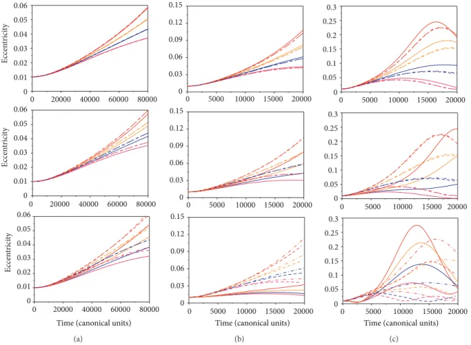
3.2. Near Critical Inclination Orbits. Figures3and4show the

results of the evolutions of the inclination and the eccentricity,

respectively, as a function of time for initial inclinations�₀=

41∘_{(red line), 40}∘_{(orange line), 39}∘_{(blue line), and 38}∘_(pink

(7)

0 0.01 0.02 0.03 0.04 0.05 0.06

Eccen

tr

ici

ty

0 0.01 0.02 0.03 0.04 0.05 0.06

Eccen

tr

ici

ty

0 20000 40000 60000 80000

0 0.01 0.02 0.03 0.04 0.05 0.06

Eccen

tr

ici

ty

0 20000 40000 60000 80000

(a)

0 0

5000 10000 15000 20000

0.03 0.06 0.09 0.12 0.15

0 0

5000 10000 15000 20000

0.03 0.06 0.09 0.12 0.15 0 0

5000 10000 15000 20000

0.03 0.06 0.09 0.12 0.15

(b)

0 0

5000 10000 15000 20000

0.05 0.1 0.15 0.2 0.25 0.3

0 5000 10000 15000 20000

0 0.05 0.1 0.15 0.2 0.25 0.3

0 0

5000 10000 15000 20000

0.05 0.1 0.15 0.2 0.25 0.3

(c)

Figure 4: hese igures show the evolution of the eccentricity as a function of time for near critical inclination spacecrat orbits. he irst,

second, and third rows correspond to the results for eccentricity of the perturbing body (��) 0.0, 0.1, and 0.2. In the irst column, the results

are for the case ofLow-altitude orbits. he second column is for the case ofMedium-altitude orbits. he third column is for the case of

High-altitude orbits. he lines are as follows: full elliptic restricted three-body problem (solid line) and single-averaged (dashed line) and

double-averaged models (dashed-dotted line). For the colors,�0 = 41∘(red line), 40∘(orange line), 39∘(blue line), and 38∘(pink line). he

increase of the semimajor axis and the eccentricity of the primaries reduce the average distance from the spacecrat to the Moon, making the perturbations stronger.

eccentricity of the primaries, so they are omitted here. It is clear that, for values of the eccentricity of the primaries up to 0.1, both averaged models are very accurate. When�� = 0.2, the single-averaged model gives more accurate results for the evolution of the eccentricity of the perturbed body, while the double-averaged model gives more accurate results for the evolution of the inclination. he increase of��also does not change the dynamics of the system in a noticeable form for low- and medium-altitude orbits. For high-altitude orbits, there is a noticeable acceleration of the dynamics.

It can be noticed that near the time 20000 canonical units, medium-altitude orbits have presented some devia-tions between the results of the full and the averaged models, in particular for the higher inclinations. his is a result of the increase of the semimajor axis from low to medium orbits, which places the spacecrat in an orbit that is much more perturbed by the third body. Again, those models begin to give results that are also not so accurate when the eccentricity of the primaries increases. It is visible that the two-second

order averaged models have results that are very closer to each other with similar deviations from the full model. So, in this range of inclinations and altitudes, both averaged models have about the same quality of results. he increases of the semimajor axis accelerate the dynamics also in this situation. Note that the time scale of the axis is diferent for low-altitude earth orbits and the deviations of the averaged models occur very early.

(8)

0 20000 40000 60000 80000 0.6

0.8 1 1.2 1.4

In

clina

tio

n (rad)

40∘

50∘

60∘

70∘

80∘

e�= 0

0 20000 40000 60000 80000

0.6 0.8 1 1.2 1.4

In

clina

tio

n (rad)

40∘

50∘

60∘

70∘

80∘

e�= 0.2

0 20000 40000 60000 80000

0.6 0.8 1 1.2 1.4

In

clina

tio

n (rad)

40∘

50∘

60∘

70∘

80∘

e�= 0.4

(a)

40∘

50∘

60∘

70∘

80∘

e�= 0.2

0.6 0.8 1 1.2 1.4

0 5000 10000 15000 20000

20000 0.6

0.8 1 1.2 1.4

40∘

50∘

60∘

70∘

80∘

e�= 0.4

0 5000 10000 15000

40∘

50∘

60∘

70∘

80∘

0.6 0.8 1 1.2 1.4

0 5000 10000 15000 20000

e�= 0

(b)

40∘ 50∘ 60∘ 70∘ 80∘

0.6 0.8 1 1.2 1.4

0 5000 10000 15000 20000

0.6 0.8 1 1.2 1.4

0 5000 10000 15000 20000 40∘

50∘ 60∘ 70∘ 80∘

e�= 0.2

0.6 0.8 1 1.2 1.4

0 5000 10000 15000 20000 e�= 0.4

e�= 0

(c)

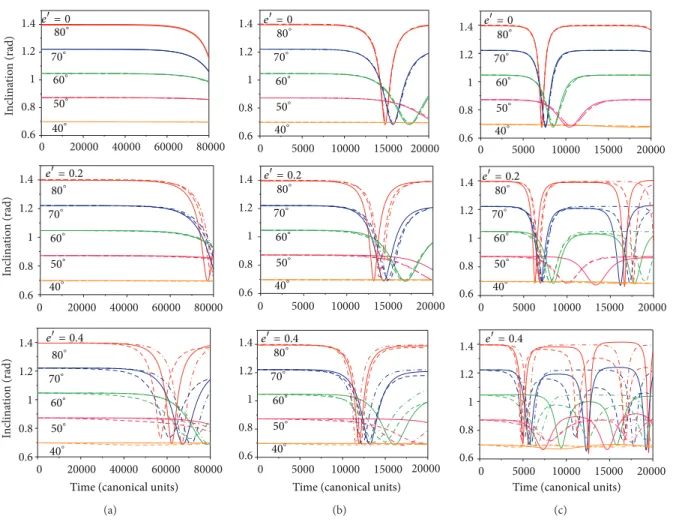
Figure 5: hese igures show the evolution of the inclination as a function of time for high-inclination spacecrat orbit. On the top of each

igure is shown the corresponding eccentricity of the perturbing body (��). In the irst column, the results are for the case ofLow-altitude

orbits. he second column is for the case ofMedium-altitude orbits. he third column is for the case ofHigh-altitude orbits. he lines are as

follows: full elliptic restricted three-body problem (solid line), single-averaged (dashed line), and double-averaged models (dashed-dotted

line). For the colors,�0= 80∘(red line), 70∘(blue line), 60∘(green line), 50∘(pink line), and 40∘(orange line). he increase of the semimajor

axis and the eccentricity of the primaries reduce the average distance from the spacecrat to the Moon, making the perturbations stronger.

the eccentricity of the primaries increases, not predicting correctly the oscillations performed by the full model. At high altitudes, both averaged approximations begin to lose quality for�� = 0.2. It is visible that the two second-order averaged models have results that are very closer to each other with similar deviations from the full model. So, in this range of inclinations and altitudes, both averaged models have about the same quality of results for values of the eccentricity of the primaries below 0.2.

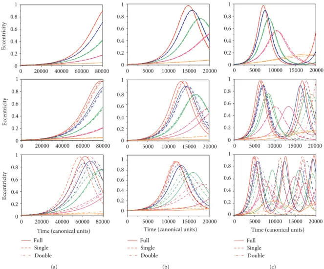
3.3. Above Critical Inclination Orbits. Figures5and6show

the evolutions of the inclinations and the eccentricities as a function of time for initial inclinations above the criti-cal value. he general behaviors are the expected ones (see [17, 18]), and the inclinations remain constant for a long time, return very fast to the critical value, and then increase again to its original values. he eccentricity shows an opposite behavior and increases when the inclination decreases and vice versa. he increase of the initial inclinations also causes oscillations with larger amplitudes. Both averaged models

have results that are excellent for��= 0.0, and they still have good accuracy for eccentricities of the primaries up to 0.2.

(9)

0 20000 40000 60000 80000 0

0.2 0.4 0.6 0.8 1

Eccen

tr

ici

ty

0 20000 40000 60000 80000

0 0.2 0.4 0.6 0.8 1

Eccen

tr

ici

ty

0 20000 40000 60000 80000

0 0.2 0.4 0.6 0.8 1

Eccen

tr

ici

ty

Time (canonical units) Full

Single

Double

(a)

0 5000 10000 15000 20000

Time (canonical units) 0

0.2 0.4 0.6 0.8 1 0 0

5000 10000 15000 20000

0.2 0.4 0.6 0.8 1 0 0

5000 10000 15000 20000

0.2 0.4 0.6 0.8 1

Full Single

Double

(b)

0 5000 10000 15000 20000

Full Single

0 5000 10000 15000 20000

Time (canonical units) 0

0.2 0.4 0.6 0.8 1

0 0.2 0.4 0.6 0.8 1

Double

(c)

Figure 6: hese igures show the evolution of the eccentricity as a function of time for high-inclination orbits. he irst, second, and third rows

correspond to the results for eccentricity of the perturbing body (��) 0.0, 0.2, and 0.4. In the irst column, the results are for the case of

Low-altitude orbits. he second column is for the case ofMedium-altitude orbits. he third column is for the case ofHigh-altitude orbits. he lines

are as follows: full elliptic restricted three-body problem (solid line), single-averaged (dashed line), and double-averaged models

(dashed-dotted line). For the colors,�0 = 80∘(red line), 70∘(blue line), 60∘(green line), 50∘ (pink line), and 40∘(orange line). he increase of the

semimajor axis and the eccentricity of the primaries reduce the average distance from the spacecrat to the Moon, making the perturbations stronger.

good for higher values of the initial inclinations, with the worst results happening for�₀ = 80∘. Another result that comes from those igures is that the increase of��causes an acceleration of the dynamics of the system. Note that the time required by the inclination and eccentricity to sufer the large-amplitude oscillation becomes shorter when the primaries are in a more elliptic orbit.

For medium altitudes, when �� = 0.4, the accuracy of the averaged models increases with the increase of the initial inclinations. Note that the averaged models are still good for the case of initial inclination 80∘, and the situation with the worst results occurs for 60∘. Inclined orbits are less perturbed by a third body because the mean distance between the spacecrat and the Moon is larger than in planar orbits.

Note that the strong changes in inclination and eccen-tricity occur earlier as a result of the stronger perturbations resulting from the increase of the semimajor axis of the orbit.

he increase of the eccentricity of the primaries has the same efect, showing that an elliptic orbit for the perturbing body causes more perturbation on the spacecrat, when compared with circular orbits with the same semimajor axis, because the distance between the bodies decreases at the periapsis. he correspondent increase of that distance at the apoapsis does not compensate the previous aspect. For values of��up to 0.2, the region where the second-order averaged models work better and the diferences between the full model and the averaged models are larger in higher orbits. his shows that the increase of the perturbation efects also increases the diferences between the models.

(10)

problem under the second-order averaged hypotheses. In general, in this situation, the single-averaged model gives better results. For�� = 0.1 and higher, the averaged models do not predict very well the time for the second jump of the inclination and eccentricity for all of the inclinations studied. he eccentricity of the primaries still accelerates the system, reducing the period of the oscillations, in the same way made by the higher altitudes. Note that, at this high altitude, the system shows two jumps for the inclination and eccentricity.

4. Conclusions

he equations of motion of a spacecrat perturbed by a third body using a single-averaged technique are developed, considering an elliptic orbit for the disturbing body.

Looking at the overall behavior, the results are according to the literature: short oscillations in the inclination and eccentricity for initial inclinations below the critical value, which increases fast in amplitude around the critical value, then the typical behavior of having the inclinations remaining constant for a long time, and then returning very fast to the critical value, to increase fast again to its original values. he eccentricity shows an opposite behavior and increases when the inclination decreases and vice versa.

he results also showed that circular orbits exist, but frozen orbits do not exist under this model. he circular orbits, in general, do not keep the inclination constant, as happened in the double-averaged model.

he increase of the semimajor axis causes an increase of the third-body perturbation, and this fact accelerates the dynamics of the system. It was noticed that the period of the oscillations of the inclination and the eccentricity are shorter when compared with lower-altitude orbits. he increase of the eccentricity of the primaries, considering the semimajor axis constant, has the same efect of accelerating the dynam-ics. So, elliptic orbits for the disturbing body have the efect of increasing the perturbation, if all other elements remain the same.

It was also showed that inclined orbits are less perturbed by a third body, since the mean distance between the space-crat and the Moon is larger than in planar orbits.

A comparison with the double-averaged technique up to the second order and with the full restricted elliptic problem was made, and it showed some other facts. he second-order averaged models are very accurate when the perturbing body is in a circular orbit. his accuracy decreases with the increase of the eccentricity of the primaries. he use of second-order averaged models is not recommended for eccentricities of the primaries of 0.3 or larger, and a better expansion, including more terms, is required in this situation. In general, both second-order averaged models have results that are much closer with each other than closer to those of the full model. It means that both averages tend to give similar errors, when compared with the full model.

Acknowledgments

he authors wish to express their appreciation for the support provided by CNPq under Contracts nos. 150195/2012-5 and

304700/2009-6, by Fapesp (contracts nos. 2011/09310-7 and 2011/08171-3), and by CAPES.

References

[1] Y. Kozai, “On the efects of the Sun and Moon upon the motion of a close Earth satellite,” Smithsonian Institution Astrophysical Observatory, Special Report 22, 1959.

[2] M. M. Moe, “Solar-lunar perturbation of the orbit of an Earth

satellite,”ARS Journal, vol. 30, no. 5, pp. 485–506, 1960.

[3] P. Musen, “On the long-period lunar and solar efects on

the motion of an artiicial satellite. II,”Journal of Geophysical

Research, vol. 66, pp. 2797–2805, 1961.

[4] G. E. Cook, “Luni-solar perturbations of the orbit of an earth

satellite,” he Geophysical Journal of the Royal Astronomical

Society, vol. 6, no. 3, pp. 271–291, 1962.

[5] P. Musen, A. Bailie, and E. Upton, “Development of the lunar and solar perturbations in the motion of an artiicial satellite,” NASA-TN D494, 1961.

[6] Y. Kozai, “Secular perturbations of asteroids with high

inclina-tion and eccentricity,”he Astrophysical Journal Letters, vol. 67,

no. 9, p. 591, 1962.

[7] L. Blitzer, “Lunar-solar perturbations of an earth satellite,”he

American Journal of Physics, vol. 27, pp. 634–645, 1959.

[8] W. M. Kaula, “Development of the lunar and solar disturbing

functions for a close satellite,”he Astronomical Journal, vol. 67,

no. 5, p. 300, 1962.

[9] G. E. O. Giacaglia, “Lunar perturbations on artiicial satellites of the earth,” Smithsonian Astrophysical Observatory, Special Report 352, 1, 1973.

[10] Y. Kozai, “A new method to compute lunisolar perturbations in satellite motions,” Smithsonian Astrophysical Observatory, Special Report 349, 27, 1973.

[11] M. E. Hough, “Lunisolar perturbations,”Celestial Mechanics and

Dynamical Astronomy, vol. 25, p. 111, 1981.

[12] M. E. Ash, “Doubly averaged efect of the Moon and Sun on a

high altitude Earth satellite orbit,”Celestial Mechanics, vol. 14,

no. 2, pp. 209–238, 1976.

[13] S. K. Collins and P. J. Cefola, “Double averaged third body model for prediction of super-synchronous orbits over long time spans,” Paper AIAA 64, American Institute of Aeronautics and Astronautics, 1979.

[14] M. ˇSidlichovsky´y, “On the double averaged three-body

prob-lem,”Celestial Mechanics, vol. 29, no. 3, pp. 295–305, 1983.

[15] J. H. Kwok, “A doubly averaging method for third body

per-turbations in planet equator coordinates,” Advances in the

Astronautical Sciences, vol. 76, pp. 2223–2239, 1991.

[16] J. H. Kwok, “Long-term orbit prediction for the venus radar

mapper mission using an averaging method,” inProceedings

of the AIAA/AAS Astrodynamics Specialist Conference, Seatle,

Wash, USA, August 1985.

[17] R. A. Broucke, “Long-term third-body efects via double

aver-aging,”Journal of Guidance, Control, and Dynamics, vol. 26, no.

1, pp. 27–32, 2003.

[18] A. F. B. A. Prado, “hird-body perturbation in orbits around

natural satellites,”Journal of Guidance, Control, and Dynamics,

vol. 26, no. 1, pp. 33–40, 2003.

[19] C. R. H. Solorzano,hird-body perturbation using a single

aver-aged model [M.S. thesis], National Institute for Space Research

(11)

[20] T. A. Ely, “Stable constellations of frozen elliptical inclined lunar

orbits,”Journal of the Astronautical Sciences, vol. 53, no. 3, pp.

301–316, 2005.

[21] T. A. Ely and E. Lieb, “Constellations of elliptical inclined

lunar orbits providing polar and global coverage,”Journal of the

Astronautical Sciences, vol. 54, no. 1, pp. 53–67, 2006.

[22] J. P. S. Carvalho, A. Elipe, R. V. de Moraes, and A. F. B. A. Prado, “Low-altitude, near-polar and near-circular orbits around

Europa,”Advances in Space Research, vol. 49, no. 5, pp. 994–

1006, 2012.

[23] J. P. D. S. Carvalho, R. V. de Moraes, and A. F. B. A. Prado, “Nonsphericity of the moon and near sun-synchronous polar

lunar orbits,”Mathematical Problems in Engineering, vol. 2009,

Article ID 740460, 24 pages, 2009.

[24] J. P. S. Carvalho, R. V. de Moraes, and A. F. B. A. Prado, “Some

orbital characteristics of lunar artiicial satellites,” Celestial

Mechanics and Dynamical Astronomy, vol. 108, no. 4, pp. 371–

388, 2010.

[25] J. P. D. S. Carvalho, R. V. de Moraes, and A. F. B. A. Prado,

“Plan-etary satellite orbiters: applications for the moon,”Mathematical

Problems in Engineering, vol. 2011, Article ID 187478, 19 pages,

2011.

[26] D. Folta and D. Quinn, “Lunar frozen orbits,” inProceedings

of the AIAA/AAS Astrodynamics Specialist Conference, AIAA

2006-6749, pp. 1915–1932, August 2006.

[27] H. Kinoshita and H. Nakai, “Secular perturbations of ictitious

satellites of uranus,”Celestial Mechanics and Dynamical

Astron-omy, vol. 52, no. 3, pp. 293–303, 1991.

[28] M. Lara, “Design of long-lifetime lunar orbits: a hybrid

ap-proach,”Acta Astronautica, vol. 69, no. 3-4, pp. 186–199, 2011.

[29] M. E. Paskowitz and D. J. Scheeres, “Design of science orbits

about planetary satellites: application to Europa,”Journal of

Guidance, Control, and Dynamics, vol. 29, no. 5, pp. 1147–1158,

2006.

[30] M. E. Paskowitz and D. J. Scheeres, “Robust capture and transfer

trajectories for planetary satellite orbiters,”Journal of Guidance,

Control, and Dynamics, vol. 29, no. 2, pp. 342–353, 2006.

[31] R. P. Russell and A. T. Brinckerhof, “Circulating eccentric orbits

around planetary moons,”Journal of Guidance, Control, and

Dynamics, vol. 32, no. 2, pp. 423–435, 2009.

[32] D. J. Scheeres, M. D. Guman, and B. F. Villac, “Stability analysis of planetary satellite orbiters: application to the Europa orbiter,”

Journal of Guidance, Control, and Dynamics, vol. 24, no. 4, pp.

778–787, 2001.

[33] C. W. T. Roscoe, S. R. Vadali, and K. T. Alfriend, “hird-body

perturbation efects on satellite formations,” inProceedings of

the Jer-Nan Juang Astrodynamics Symposium, AAS Preprint No

12-631, College Station, Tex, USA, June 2012.

[34] R. C. Domingos, R. V. de Moraes, and A. F. B. A. Prado, “hird-body perturbation in the case of elliptic orbits for the disturbing

body,”Mathematical Problems in Engineering, vol. 2008, Article

ID 763654, 14 pages, 2008.

[35] X. Liu, H. Baoyin, and X. Ma, “Long-term perturbations due

to a disturbing body in elliptic inclined orbit,”Astrophysics and

Space Science, vol. 339, no. 2, pp. 295–304, 2012.

[36] R. C. Domingos, R. V. de Moraes, and A. F. B. A. Prado, “hird-body perturbation in the case of elliptic orbits for the disturbing

body,” inProceedings of the AIAA/AAS Astrodynamics Specialist

Conference, Mackinac Island, Mich, USA, August 2007.

[37] R. C. Domingos, R. V. de Moraes, and A. F. B. A. Prado, “hird body perturbation using a single averaged model considering

elliptic orbits for the disturbing body,”Advances in the

Astro-nautical Sciences, vol. 130, p. 1571, 2008.

[38] C. D. Murray and S. F. Dermott,Solar System Dynamics,

(12)

Submit your manuscripts at

http://www.hindawi.com

Hindawi Publishing Corporation

http://www.hindawi.com Volume 2014

Mathematics

Journal of

Mathematical Problems in Engineering

Hindawi Publishing Corporation http://www.hindawi.com

Differential Equations International Journal of

Volume 2014

http://www.hindawi.com Volume 2014 Mathematical PhysicsAdvances in

Complex Analysis

Journal of

Optimization

Journal of

Combinatorics

http://www.hindawi.com Volume 2014 International Journal of Hindawi Publishing Corporation

Journal of

Function Spaces

Abstract and Applied Analysis Hindawi Publishing Corporation

International Journal of Mathematics and Mathematical Sciences

Hindawi Publishing Corporation http://www.hindawi.com Volume 2014

The Scientiic

World Journal

Discrete Dynamics in Nature and Society Hindawi Publishing Corporation

Discrete Mathematics

Journal of

http://www.hindawi.com Volume 2014 Hindawi Publishing Corporation