Effects of the Eccentricity of a Perturbing Third Body on the Orbital Correction Maneuvers of a Spacecraft

(1)

Research Article

Effects of the Eccentricity of a Perturbing Third Body on the

Orbital Correction Maneuvers of a Spacecraft

R. C. Domingos,

1,2

A. F. B. A. Prado,

2

and V. M. Gomes

3 1_{Universidade Estadual Paulista (UNESP), S˜ao Jo˜ao da Boa Vista, SP, Brazil}

2_{Instituto Nacional de Pesquisas Espaciais (INPE), 12227-010 S˜ao Jos´e dos Campos, SP, Brazil}

3_{Universidade Estadual Paulista (UNESP),12516-410 Guaratinguet´a, SP, Brazil}

Correspondence should be addressed to R. C. Domingos; rdomingos95@gmail.com

Received 25 January 2014; Revised 21 April 2014; Accepted 17 May 2014; Published 3 July 2014

Academic Editor: Maria Cecilia Zanardi

Copyright © 2014 R. C. Domingos et al. his is an open access article distributed under the Creative Commons Attribution License, which permits unrestricted use, distribution, and reproduction in any medium, provided the original work is properly cited.

he fuel consumption required by the orbital maneuvers when correcting perturbations on the orbit of a spacecrat due to a perturbing body was estimated. he main goals are the measurement of the inluence of the eccentricity of the perturbing body on the fuel consumption required by the station keeping maneuvers and the validation of the averaged methods when applied to the problem of predicting orbital maneuvers. To study the evolution of the orbits, the restricted elliptic three-body problem and the single- and double-averaged models are used. Maneuvers are made by using impulsive and low thrust maneuvers. he results indicated that the averaged models are good to make predictions for the orbital maneuvers when the spacecrat is in a high inclined orbit. he eccentricity of the perturbing body plays an important role in increasing the efects of the perturbation and the fuel consumption required for the station keeping maneuvers. It is shown that the use of more frequent maneuvers decreases the annual cost of the station keeping to correct the orbit of a spacecrat. An example of an eccentric planetary system of importance to apply the present study is the dwarf planet Haumea and its moons, one of them in an eccentric orbit.

1. Introduction

Advances in astronomy have been showing a large number of planets outside the solar system, some of them in orbits with large eccentricities. In that sense, it would be interesting to know how oten and how expensive would it be to keep the most important orbital elements (inclination and eccentricity) inside deined limits for a satellite orbiting one of those planets and perturbed by the central star, or even for a satellite orbiting a moon of those planets. he Solar System also has some examples of bodies with large eccentricity, like the dwarf planet Haumea and one of its moons [1]. his body belongs to the Kuiper belt and has a moon (Namaka) with eccentricity of 0.249, which is near the limit where the method shown here is valid. So, there are many possible applications of the ideas developed here. he study is made using the eccentricity of the perturbing body as a parameter, because our goal is to explore how much this eccentricity afect the orbit of the satellite. It is possible to see that, for

some values of the eccentricity, no orbital maneuvers are required for longer time, in the order of decades.

An orbital maneuver is a procedure performed with the goal of modifying the orbit of a satellite by using a propulsive system ixed to the spacecrat, which is able to modify the velocity of the spacecrat and, consequently, its orbit. his procedure can be used when inserting a satellite in its inal orbit from a previous parking orbit where the launcher was able to deliver it, or to correct the deviations from the nominal orbit due to the action of perturbation forces. One of the irst results in this ield is the so-called Hohmann transfer [2]. It considers the transfer with minimum variation of velocity between two coplanar and circular orbits. Later, the three-impulsive concept appeared in the literature, in independent researches developed by Hoelker and Silber [3] and Shternfeld [4]. In this maneuver, a bielliptical three-impulsive transfer between two circular orbits has a lower variation of velocity than the one required by the Hohmann transfer if the ratio between the initial and inal radius of

(2)

the orbits is greater than 15.48. In the range from 11.94 to 15.58, the more economical maneuver can use two or three impulses, depending on the value of the distance where the second impulsive is applied (see Marec [5]).

he next step is to consider whether a low thrust can be used to maneuver the satellite. In this situation, the propulsion system applies a inite force for a nonnegligible time. Many researches using this model are based directly on the “Primer-Vector” theory, which was developed by Lawden [6, 7]. Other strategies to solve this problem are based on Pontryagin’s maximum principle. Biggs [8, 9] and Gomes and Prado [10] show some results using this technique in researches that are the basis of the procedure used in the present paper when the low thrust maneuvers are considered. he present paper makes use of both types of maneuvers cited above to correct the perturbations from a third-body in an elliptical orbit. It is important to note that the amplitudes of the maneuvers performed here are small, because it is only required to make the satellite to return to its nominal orbit, correcting the efects of the third-body perturbation. hus, an initial and a inal orbit around the Earth are given and the goal is to search for solutions on how to transfer the satellite between those two orbits, which presents a low cost in terms of fuel consumption. In that sense, this is an orbital maneuver between two close near circular orbits. Previous researches made in this problem can be found by Marec [11], Edelbaum [12], Fernandes and Golfetto [13], Fernandes and Carvalho [14], and Fernandes [15].

In this way, the present research concentrates on studying the time evolution of a satellite perturbed by a third-body, for times of the order of a few tens of years, under the single-and double-averaged models, to compare their results with the full elliptic restricted three-body problem, that will be our “full model” to represent the reality. hese irst results give an idea of the diferences between those models in this time span, which is chosen to cover times larger than the usual spacecrat missions around the Earth. hose larger times can include missions like a permanent basis orbiting an exoplanet in an elliptic orbit around a central star or a “temporary” spacecrat orbiting asteroids in eccentric orbits. A spacecrat placed in orbit around Haumea would also beneit from those previous studies. Missions like those ones have a good potential to require duration of the order of 20–30 years. Another result of this research is to ind the times when it is necessary to perform orbital maneuvers to send the satellite back to its nominal orbit, thus correcting the variations introduced by the presence of the third-body. hese calculations are based on the instants that the satellite reaches one of the accepted limits of the mission for the deviations in eccentricity and/or inclination. Since the corrections in the inclination are made by out-of-plane maneuvers and the corrections in eccentricity are made by planar maneuvers, both corrections are assumed to be made independently of each other. Two diferent approaches are used for both situations, in order to compare the cost involved: an impulsive maneuver that is easier to calculate and is usually considered as a irst model for almost all mission designers and a low thrust transfer that has the advantage of using less fuel to achieve the same inal orbit, due

to the higher value of the speciic impulse, but requires a more complex implementation of the hardware used to control the system.

2. Mathematical Models

In order to study the maneuvers to control eccentricity and inclination due to the perturbations caused by a third-body in an elliptical orbit, the assumptions used to develop the single-and double-averaged analytical models are the same ones of the restricted elliptic three-body problem. It is assumed that a planet with mass�₀is ixed in the center of the reference system �-�. he perturbing body, with mass ��, is in an elliptic orbit with semimajor axis��, eccentricity��, and mean motion��. he satellite with mass�that can be considered negligible when compared to the other masses involved is in a generic orbit whose orbital elements are�(semi-major axis),

�(eccentricity),�(inclination),�(argument of periapsis), and

Ω(right ascension of the ascending node). Its mean motion, obtained from its semimajor axis, is called�. he reason to develop averaged models is that they can be used to show the behavior of the orbit in longer time periods, by removing short term oscillations that may not be important in some studies. Using this technique, it is possible to obtain analytical equations of motion that can be analyzed to show some characteristics of the motion and that can also be integrated to give fast results in terms of the long period evolution of the orbital elements.

(3)

2.1. Single-Averaged Model. In Domingos et al. [16],Section 2, a complete review and more details about the development of the disturbing potential and the average process are shown.

he equations of motion are used as in Domingos et al. [17] to compute the efects of the perturbing body on the satellite. Using an expansion in Legendre’s polynomials (considering��≫ �), the second order part of the disturbing potential, considering an average over the eccentric anomaly of the satellite, is given by

⟨�2⟩ = �

�_�2_��2

2 (�

�

��)

3

× {(1 + 32�2

) [32 (�2_{+ �}2_{) − 1]}

+154 (�2_{− �}2_{) �}2_{} ,}

(1)

where �� = ��(1 − ��2)/(1 + ��cos��), cos�� = cos��

+ ��(cos2�� − 1) + (9/8)��2(cos3�� − cos��) + ⋅ ⋅ ⋅,

and sin�� = sin�� + ��sin2�� + ��2((9/8)sin3�� −

(7/8)sin��)+⋅ ⋅ ⋅.

When considering elliptic orbits for the perturbing body, the values of � and � are given by � = cos�cos� −

cos�sin�sin�, � = −sin�cos� − cos�cos�sin�, and

� = Ω − ��_{− �}�_{. he mean anomaly of the perturbing body}

��_{is given by}_�� _{= �}�

�+ ��. hus, the variations in the

orbital elements of the perturbed body are obtained. To do this, we derived Lagrange’s planetary equations that describe the variations of the mean orbital elements of the spacecrat. hey are given by

�� = −

(1 − �2₎1/2

��2_� � ⟨�⟩_{�� ,}

��

�� = sin�[�� (1 − �cos� 2)]1/2

� ⟨�⟩ ��

− 1

sin�[�� (1 − �2)]1/2

� ⟨�⟩ �Ω ,

�Ω

�� = sin�[�� (1 − �1 2)]1/2

� ⟨�⟩ �� ,

��

�� = − sin�[�� (1 − �cos� 2)]1/2

� ⟨�⟩ �� +

(1 − �2₎1/2

��2_� � ⟨�⟩_{�� .}

(2)

he semimajor axis is constant since the mean anomaly

�was eliminated in the perturbing function. Following this idea, we numerically integrate the equation of motion (3),

obtained from Lagrange’s planetary equations. he results are shown below:

��

�� = �154 ��2�√1 − �

2

�

× [sin2� (cos2� −cos2�sin2�)

−cos�cos2�sin2�] ,

��

�� = �sin�[�� (1 − �1 2)]1/2

3

4��2�2

× {�2[−5cos2�sin2�cos2�

+ 32 (−sin2�+sin2�cos2�)

− 52sin�cos2� (1 +cos2�)]

+ (sin� −sin2�cos2�)

− 5cos2�sin2�cos�} ,

�Ω

�� = �34��2 �

2

sin�[�� (1 − �2)]1/2

× {(1 + 32�2_{) (−}_sin2_�_sin_2�)

+ [cos2�cos2�sin2� +sin�sin2�sin2�]

× (52�2)} ,

��

�� = �34��2

× {− �2

sin�[�� (1 − �2)]1/2

× [(1 + 32�2) (−sin2�sin2�)

+ (52�2_{) (}_cos_2�_sin2_�_cos_2�)

+ 12sin2�sin2�sin2�]

+√1 − �_� 2[5 (cos2� −cos2�sin2�)cos2�

− 5cos�sin2�sin2�

+ 62 (cos2� +cos2�sin2�)]} ,

(3)

(4)

his set of equations has singularities for equatorial orbits, because the inclination appears in the denominator of some of them. here is no singularity for small eccentricities, because it does not appear in the denominator. So, it is necessary to check the results very carefully against the other models, which have no singularities, when near equatorial orbits are considered. In any case, exactly equatorial orbits were not used in the present research.

2.2. Double-Averaged Model. Using (1) and considering an average over the eccentric anomaly of the perturbing body (Domingos et al. [16]), the equation obtained for the double-averaged disturbing function is

⟨⟨�2⟩⟩ = ��[2 (3cos2� − 1) + 3�2(3cos2� − 1)

+15�2_sin2_�_cos_{2�] .} (4)

Now, it is possible to quantify the resulting variations in the orbital elements of the satellite. To obtain this result, again Lagrange’s planetary equations are derived using the perturbing potential shown by (4). he results are given by

��

�� = ��15�

�_��2_{�√1 − �}2

8� sin2(�)sin(2�) ,

��

�� = ��−15�

�_��2_�2

16�√1 − �2 sin(2�)sin(�) ,

��

�� = �� 3�

�_��2

8�√1 − �2[(5cos

2_{(�) − 1 + �}2₎

+5 (1 − �2₋_cos2_(�))_cos_{(2�)] ,}

�Ω

�� = ��3�

�_��2_cos_(�)

8�√1 − �2 [5�

2_cos_{(2�) − 3�}2_{− 2] ,}

��

�� = − ��

�_��2

8� [(3�2+ 7) (3cos2(�) − 1)

+15 (1 + �2)sin2(�)cos2(�)] ,

(5)

where��= [1 + (3/2)��2+ (15/8)��4].

his set of equations has no singularities, so it is important to use it to verify the results obtained by the previous method, in particular when near equatorial orbits are considered.

2.3. he Impulsive Transfers to Correct the Eccentricity. In present study, we have considered the time evolution and maneuvers to correct only inclination and eccentricity, because they were considered the most important elements that impact the orbit of the satellite (see [13,14]). As shown by the mathematical models used here, the semimajor axis is not afected by third-body perturbations, except for short periodic oscillations of small amplitudes. he argument of periapsis and the right ascension of the ascending node do not afect very much the mission under analysis, since they do not change the regions of the celestial body that is covered by the satellite. hose variables have a secular perturbation

ΔV2 ΔV1

OT

O2

O1

X Y

ra2

rp1

Figure 1: Geometry of the bi-impulsive transfer.

that causes a circular motion for both angles (Sol´orzano and Prado [20]).

To return the eccentricity of an orbit to its original value and keeping the same semimajor axis, one possibility is to make a bi-impulsive transfer to send the satellite from an orbit O₂, with a given semi-major axis “�” and eccentricity “�₂”, to an orbit O₁, with the same semimajor axis “�” but with eccentricity “�₁”. Another possibility would be to perform a single impulsive maneuver at the point where the orbits intersect each other. he two-impulsive maneuver will be used, because it uses the apsis of the orbits, which are better in terms of fuel consumption, and also because splitting the maneuver in two parts makes the task of correcting errors in the impulses applied easier. Since the semimajor axis is not changed by the third-body perturbations, in terms of average, it is also desired to perform orbital maneuvers that do not change this parameter. So, when correcting the eccentricity, this is the only orbital parameter that needs to be changed by the maneuver.Figure 1shows this situation. A good solution is a Hohmann type transfer that uses the most distant apoapsis. So, it is necessary to apply the irst impulse, with magnitudeΔ�₁, to the satellite when it is at the apoapsis of the orbit O₂that is a point where the distance from the center of the Earth is�_�2. his impulse puts the satellite in a transfer orbit O_�that is an ellipse tangent to the apoapsis of O₂and to the perigee of O₁, where the distance from the center is�_�1. When the satellite reaches the periapsis of the orbit O₁, the second impulse, with magnitudeΔ�₂, is applied to the satellite and this impulse puts the satellite in the inal desired orbit O₂. his second impulse is applied opposite to the direction of the motion of the satellite, in order to remove energy from the satellite, thus returning its semimajor axis to the original value.

To obtain the magnitude of the impulses, it is possible to start with the vis viva equation (6), where Vis the velocity

of the satellite,�is the distance between the satellite and the center of the Earth, and�is the gravitational parameter of the Earth, whose numerical value used here is 398600 km3/s2:

V= √ 2�

(5)

Based on that equation, the magnitude of the irst impulse is the diference between the velocity of the satellite when it is at the point�_�2in the orbit O₂and the velocity when the satellite is at the same point but in the orbit O_�. he equation is

Δ�1= √_{� (1 − �}2� 2₎− �_�_� − √_{� (1 − �}2� 2₎− ��, (7)

where�_�is the semimajor axis of the transfer orbit O_�, which is given by

��= � + �2 (�2− �1) . (8)

he second impulse is applied at the periapsis of the nominal orbit and it is in the opposite direction with respect to the motion of the satellite, thus reducing the energy and the semimajor axis of the orbit to return it to its original value. Its magnitude is the diference between the velocities of the satellite at this point when it is in the orbit O_�and its velocity at the same point but when the satellite is at the orbit O₂. he equation is

Δ�2= √_{� (1 − �}2� 2

1)− �� − √

2�

� (1 − �2

1)− ��. (9)

he total variation of velocity required by the maneuver is given byΔ�_� = Δ�₁+ Δ�₂. he conversion to get the fuel mass consumed is obtained from the well-known Tsiolkovskii equation [21]:

�0= ��(Δ��/�0�sp), (10)

where�₀ is the acceleration of gravity at the surface of the Earth, assumed to be 9.8 m/s2;�spis the speciic impulse of the engine (considered to be 340 s); the subscript�assumes the values 1 and 2 to represent both impulses;�₀is the mass of the satellite before the impulse; and �_� is the mass of the satellite ater the impulse, such that�₀− �_�is the fuel consumed by the maneuver. So, it is necessary to have a value for the initial mass of the satellite and the parameters of the combination engine/fuel in order to obtain the total consumption in terms of fuel mass. his equation is used for both impulses separately, updating the value of the mass ater the irst impulse, not toΔ�_�, to get more accuracy.

2.4. he Impulsive Transfer to Correct the Inclination. In this situation, the simplest strategy is to make a single impulsive transfer to rotate the velocity of the satellite by the desired angle. his impulse has to be applied when the satellite passes by the intersection of the two planes: the one where the satellite is orbiting and the one where it should go ater the maneuver. he magnitude of this impulse is given by [22]

Δ��= 2Vsin(Δ�2), (11)

whereVis the velocity of the satellite at the moment of the

application of the impulse andΔ�is the plane change required

by the maneuver. Since the nominal orbit is not circular, the magnitude of this impulse depends on the true anomaly of the point of the application of the impulse, which depends on the geometry of the problem (values of the argument of the periapsis and the right ascension of the ascending node) and how the perturbation changes those variables. To avoid speciic cases and considering that the eccentricity is small so that the magnitude of the velocity does not oscillate too much, it is possible to consider the worst case, which is when making the maneuver at the periapsis of the orbit, the point where the velocity is larger. In this case, the maximum velocity variation required by the maneuver that changes the inclination (Δ�max) is given by

Δ��max= 2sinΔ�

2 √� (1 − �2� 2

1)− ��. (12)

his equation is obtained just by replacing the term in velocity by the velocity at periapsis. he conversion to fuel mass is obtained once again by using (10).

2.5. Low hrust Maneuvers. he same transfers described above can be performed using low thrust. he reason to do that is the smaller fuel consumption required by the low thrust propulsion system, due to its higher speciic impulse. It is assumed that the satellite can arrive and leave at any point in the inal and initial orbits, respectively. he maneuver is assumed to be realized by an engine that delivers a thrust with variable direction and constant magnitude.

(6)

4

3

2

1

0

Dir

ec

tio

n

o

f t

h

ru

st (deg)

−6 −4 −2 0 2 4 6

True anomaly (deg)

(a)

180

179

178

177

176

Dir

ec

tio

n

o

f t

h

ru

st (deg)

174 176 178 180 ₁₈₂ 184 186

True anomaly (deg)

(b)

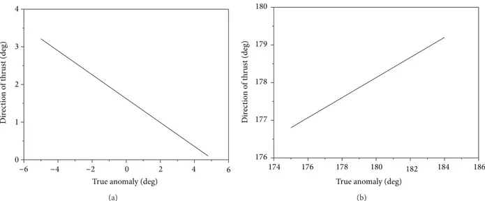
Figure 2: Low thrust to correct the eccentricity for the maneuver from 0.02 to 0.01 using two arcs of propulsion.

thus changing it from 0.02 to 0.01. he other situations are similar, so only the fuel consumption and the duration of the maneuvers are shown in the tables and the igures are omitted. he duration of the application of the thrust is short, so the plots of the trajectories are not interesting, since they are Keplerian orbits. Ater that, the errors of the propulsion system were considered, using a very simple approach. he solution is obtained as a set of points, which represents the whole trajectory. hen, we inserted a ixed error in the magnitude (5%) and in the direction of the solution obtained (2 degrees) at every point obtained as a solution of the maneuver. he constraints of reaching the inal orbit speciied were the same of the maneuvers without errors. So, using this simple approach, it was possible to see that the errors in the fuel consumed were in the order of 5–7%. his result is expected because the maneuvers have small magnitudes and so there is an almost linear dependence between errors and extra consumption.

3. Results

Based on the mathematical models described in the previous sections, performed some numerical simulations are now performed using (3), for the single-averaged model, and (5), for the double-averaged model, to verify the evolution of the eccentricity and inclination due to the third-body pertur-bations for high-altitude circular orbits (semimajor axis of 42284 km). hese orbits have the altitude of the geostationary orbits around the Earth, and they are chosen because they have strong efects from the third-body perturbations. hus, the choice of high-altitude orbits in addition to the system with mass parameters equivalent to the Earth-Moon system with variable eccentricity can better show the validity of the results presented. Near equatorial (�₀ = 10−3 degrees), near the critical inclination of the third-body perturbation (�₀ =

39∘_{∼ 0.6803}_{radians), and high inclined orbits (}_�

0 = 80∘ ∼

1.3955radians) are used for the simulations. he initial orbit

of the satellite is assumed to have eccentricity �₀ = 0.01 and right ascension of the ascending node and argument of periapsis equal to zero.

3.1. Finding the Consumptions and the Durations of the Maneuvers. Ater verifying the evolution of the eccentricity and inclination for∼35 years (near 478 orbits of the perturb-ing body), it is possible to obtain the exact times where those variables reach the limits of variation accepted by the mission from the original orbit of the satellite. Several values are used for those limits of variation for the eccentricity,Δ�, and for the inclination,Δ�, thus studying the inluence of this parameter. hose parameters represent diferent requirements that can be made by diferent missions. he values used are 0.0005, 0.001, 0.005, 0.01, 0.02, and 0.05 forΔ�and 0.0001, 0.0005, 0.001, and 0.005 radians forΔ�. When those limits are reached (�₀ ± Δ�and/or �₀ ± Δ�), a maneuver is used to return the satellite to its original orbit. he evolutions of the eccentricity and the inclination are shown in Figures3to5.

As shown in Section 2, considering the instantaneous propulsive system, the maneuvers used to correct the devi-ations in eccentricity are the bi-impulsive planar version and the maneuver used to correct the inclination is the single impulsive maneuver. When the low trust system is considered, the maneuver to correct the errors in eccentricity is performed under two diferent hypotheses: with one or two propulsion arcs. he same system corrects the errors in inclination, but now using only one propulsion arc. Tables

(7)

0 5 10 15 20 25 30 35 0.0095

0.0100 0.0105 0.0110 0.0115

Time (year)

0 5 10 15 20 25 30 35 Time (year)

e

0.0095 0.0100 0.0105 0.0110 0.0115

e

e󳰀= 0

e󳰀= 0.1

e󳰀= 0.2

0.025

0.020

0.015

0.010

(a)

0 5 10 15 20 25 30 35 Time (year)

0.0095 0.0100 0.0105 0.0110 0.0115

e

0.0095 0.0100 0.0105 0.0110 0.0115

e

0.0095 0.0100 0.0105 0.0110 0.0115

e

(b)

0 5 10 15 20 25 30 35

Time (year)

0 5 10 15 20 25 30 35 Time (year)

0.0095 0.0100 0.0105 0.0110 0.0115

e

0.0095 0.0100 0.0105 0.0110 0.0115

e

0.0095 0.0100 0.0105 0.0110 0.0115

e

(c)

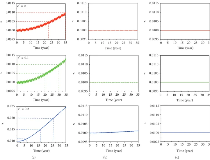
Figure 3: hese igures show the evolution of the eccentricity as a function of time for near equatorial orbits. he eccentricity of the perturbing body (��) is shown in color codes: 0.0 (red), 0.1 (green), and 0.2 (blue). In (a), the results are for the full elliptic restricted three-body problem. (b) is for single-averaged model and (c) is for double-averaged model. he dashed curve represents the (�,�) pair to perform orbital maneuvers, depending on the limit of the eccentricity variation allowed by the mission.

he low thrust maneuvers are obtained from the algorithm described in [10].

To obtain the mass of fuel required by each maneuver, as an example, a satellite with an initial mass of 1000 kg is used. he hydrazine is assumed to be the fuel for the impulsive maneuvers, with �sp = 340 seconds. For the low thrust maneuvers, a force of 10 newtons and a speciic impulse of the 1300 s were used for the propulsive system.

he durations of the propulsion arcs were not too large, going from about 0.2 minutes to nearly 21 minutes, depending on the amplitude of the maneuver. Since all the corrections are small, the consumptions are nearly proportional to the amplitudes of the maneuvers. he maneuvers using two propulsion arcs divide the fuel consumption near equally between two arcs, sometimes showing a little larger con-sumption in the irst thrusting arc, because this arc has distances to the Earth that are a little smaller, so it spends more fuel for the maneuver. Anyway, these diferences in distances from the Earth are too small and not always implied in diference in consumption between both arcs considering

(8)

0.0 0.1 0.2

Time (year) 0.005

0.010 0.015 0.020 0.025 0.030

e

0 500 1000 1500 2000 2500 3000

0 5 10 15 20 25 30 35 Time (year)

0.6790 0.6795 0.6800 0.6805

i

(rad)

(a)

0.005 0.010 0.015 0.020 0.025 0.030

e

0 5 10 15 20 25 30 35 Time (year)

0.0 0.1 0.2

0 5 10 15 20 25 30 35 Time (year)

i

(rad)

0.6780 0.6785 0.6790 0.6795 0.6800 0.6805

(b)

0.0 0.1 0.2 0.005 0.010 0.015 0.020 0.025 0.030

e

0 5 10 15 20 25 30 35 Time (year)

i

(rad)

0.6780 0.6785 0.6790 0.6795 0.6800 0.6805

(c)

Figure 4: Evolution of the eccentricity and inclination as a function of time for the case�₀= 39∘(∼0.6803 radians). In (a), the results are for the full elliptic restricted three-body problem. (b) is for the single-averaged model and (c) is for the double-averaged model. he eccentricity of the perturbing body (��) is shown in color codes: 0.0 (red), 0.1 (green), and 0.2 (blue). he dashed curves represent the (�,�) and (�,�) pairs for eccentricity and inclination, respectively, to perform orbital maneuvers, depending on the limit of the eccentricity and inclination variations allowed by the mission. In the plots for the inclination, it showed the dashed lines for the limits of variation for times higher than 1 year for better graphic visibility.

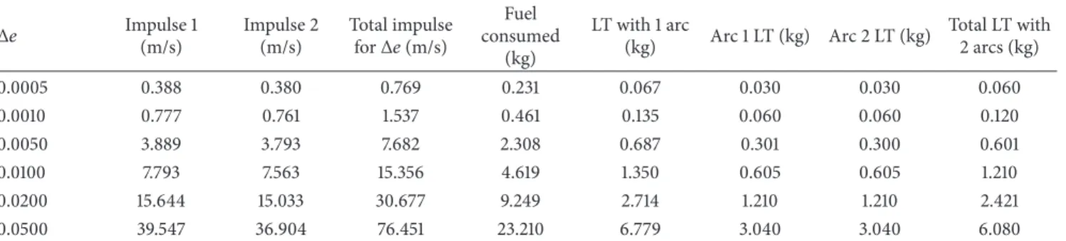
Table 1: Fuel consumption for the maneuvers to correct the eccentricity.

Δ� Impulse 1_(m/s) Impulse 2_(m/s) Total impulse_for_Δ�_(m/s) consumedFuel (kg)

LT with 1 arc

(kg) Arc 1 LT (kg) Arc 2 LT (kg)

Total LT with 2 arcs (kg)

0.0005 0.388 0.380 0.769 0.231 0.067 0.030 0.030 0.060

0.0010 0.777 0.761 1.537 0.461 0.135 0.060 0.060 0.120

0.0050 3.889 3.793 7.682 2.308 0.687 0.301 0.300 0.601

0.0100 7.793 7.563 15.356 4.619 1.350 0.605 0.605 1.210

0.0200 15.644 15.033 30.677 9.249 2.714 1.210 1.210 2.421

0.0500 39.547 36.904 76.451 23.210 6.779 3.040 3.040 6.080

Table 2: Time required by the low thrust maneuvers to correct the eccentricity.

Limit reached forΔ� hrusting time Arc 1 (min)

hrusting time for Arc 2 (min)

hrusting time with 2 arcs (min)

hrusting time with 1 arc (min)

0.0005 0.094 0.094 0.188 0.210

0.0010 0.188 0.188 0.376 0.419

0.0050 0.940 0.938 1.878 2.091

0.0100 1.89 1.89 3.78 4.22

0.0200 3.781 3.781 7.562 8.439

(9)

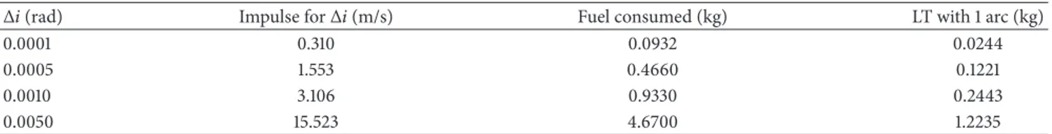
Table 3: Fuel consumption for the maneuvers to correct the inclination.

Δ�(rad) Impulse forΔ�(m/s) Fuel consumed (kg) LT with 1 arc (kg)

0.0001 0.310 0.0932 0.0244

0.0005 1.553 0.4660 0.1221

0.0010 3.106 0.9330 0.2443

0.0050 15.523 4.6700 1.2235

0 5 10 15 20 25 30 35

Time (year) 0.12

0.10

0.08

0.06

0.04

0.02

0.00

e

0.0

0.1 0.2

Figure 5: Evolution of the eccentricity as a function of time for the case�₀ = 80∘ (∼1.3955 radians). he results are for the full elliptic restricted three-body problem. Similar results have been obtained for single- and double-averaged models. he eccentricity of the perturbing body (��) is shown in color codes: 0.0 (red), 0.1 (green), and 0.2 (blue). he dashed curves represent the (�,�) pair to perform orbital maneuvers for each limit assumed for the variation in eccentricity.

Table 4: Time required by the low thrust maneuvers to correct the inclination.

Δ�(rad) hrusting time (min)

0.0001 0.085

0.0005 0.426

0.0010 0.852

0.0050 4.270

arc. he reason for these extra savings is the application of the thrust in the regions where they are more eicient, that is, the apoapsis of the trajectories involved. At those points, the gravitational force of the Earth is smaller, thus allowing larger efects due to the application of the thrust.

Tables3and4show the equivalent results of the maneu-vers used to correct the inclination. hose maneumaneu-vers require less fuel than the ones to correct eccentricities, because the limits to perform an orbital correction are very small for the inclination. he fuel consumption goes from 0.0244 to 1.2235 kg and the duration of the propulsion goes from 0.08 to 4.27 minutes. here is an almost linear relation between

the desired angle change and the fuel consumption, due to the small values involved in the variations of the inclination. In this situation, only one propulsion arc was used for each maneuver, since it is the best solution, even for the impulsive maneuvers.

3.2. Near Equatorial Orbits. Figure 3shows the evolution of the eccentricity as a function of time for the near equatorial orbits (�₀ = 10−3 degrees, since real equatorial orbits show singularities in the single-averaged equations of motion). he times are shown in years. Figures3(a),3(b), and3(c) show the results of the cases of the full elliptic restricted problem and single- and double-averaged models, respectively. On the top of each igure, the corresponding eccentricity of the perturbing body (��) is shown. his parameter is used in order to study its efects on this problem and it represents the same system used before. It is clear that none of the speciied limits is reached when using the single-averaged and the double-averaged techniques (see Figures 3(b) and

3(c)). he similar results, in terms of reaching the limits to make a maneuver, which comes from both averaged models, are expected because both averaged models have results that are very close to each other when the perturbing body is in a circular orbit (Domingos et al. [17]). his efect decreases with the increase in the eccentricity of the primaries. In general, both averaged models have results that are much closer to each other than closer to those of the full model. It is visible from the full model that, during the integration time, the evolution of the eccentricity has oscillations that increase in amplitude with the increase in the eccentricity of the primaries. he averaged models are not able to predict this property. his fact changes the times when the maneuvers are required, so it has a strong inluence on the estimation of the fuel consumption for the station keeping maneuvers.

On the other hand, the results show that, for the full elliptic restricted three-body problem, in Figure 3(a), the limits of variation of the eccentricity 0.0005, 0.001, 0.005, and 0.01 are reached, so it is necessary to perform orbital maneuvers. As an example, inFigure 3(a), we can see that

when�� = 0.2only the limit of variation for the eccentricity

Δ� = 0.05 is not reached during the timescale of the

numerical integrations. As a result, in this latter case, we do evidence that there are four points where it is required to perform orbital maneuvers to correct the orbit. he inclinations have zero variations during this period, so it is not required to apply any propulsion system to correct the orbit. For cases with�� < 0.2, the results shown inFigure 3

(10)

Table 5: Times when the limits are reached and fuel consumption per year of mission.

Eccentricity of the perturbing body Time to reach theΔ�andΔ�limits (year) Yearly consumption for impulsive maneuvers (kg)

��_{= 0.0} Δ� = 0.0005 full model = 22.82 0.0101

Δ� = 0.001 full model = 34.78 0.0133

��_{= 0.1} Δ� = 0.0005 full model = 19.93 0.0116

Δ� = 0.001 full model = 29.95 0.0154

��_{= 0.2}

Δ� = 0.0005 full model = 4.76 0.0485

Δ� = 0.001 full model = 6.71 0.0687

Δ� = 0.005 full model = 16.62 0.1389

Δ� = 0.01 full model = 26.08 0.1771

Table 6: Times when the limits are reached and average yearly fuel consumption for the mission.

Eccentricity of the

perturbing body Time to reach theΔeandΔilimits (year)

Yearly consumption for impulsive maneuvers (kg)

Fore�= 0.0

full model = 5.50

Δ� = 0.0005 single averaged model = 5.75

double averaged model = 5.76 full model = 7.63

double averaged model = 22.92

0.0420 0.0402 0.0401 0.0604 0.0560 0.0559 0.1274 0.1147 0.1146 0.1650 0.1476 0.1476 7.7667 0.9320 0.0041

Fore�= 0.1

full model = 8.77

0.0263 0.0406 0.0407 0.0359 0.0568 0.0568 0.0745 0.1164 0.1163 0.0150 0.0150 7.7667 1.1229 0.0036

Fore�= 0.2

full model = 13.64

(11)

Table 7: Times when the limits are reached and the average yearly fuel consumption for the mission assuming a circular orbit for the perturbing body.

Limit reached Time to reach the limit (year)

Δ� = 0.0005 Full model = 3.69Single-averaged model = 3.65

Double-averaged model = 3.64

0.0626 0.0633 0.0635

0.0899 0.0893 0.0893

0.2017 0.1985 0.1985

0.2885 0.2816 0.2815

0.4168 0.04074

0.4073

0.7172 0.6991 0.6989

7.7667 7.7667 0.0031

Δ� = 0.0005 Full model = 29.98_{Single-averaged model = 32.15} 0.0155_0.0145

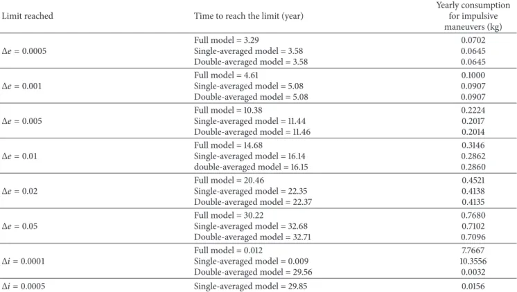
Table 8: Times when the limits are reached and the fuel consumption per year of mission using the value of 0.1 for the eccentricity of the orbit of the perturbing body.

0.0702 0.0645 0.0645

0.1000 0.0907 0.0907

0.2224 0.2017 0.2014

double-averaged model = 16.15

0.3146 0.2862 0.2860

0.4521 0.4138 0.4135

0.7680 0.7102 0.7096

7.7667 10.3556

0.0032

(12)

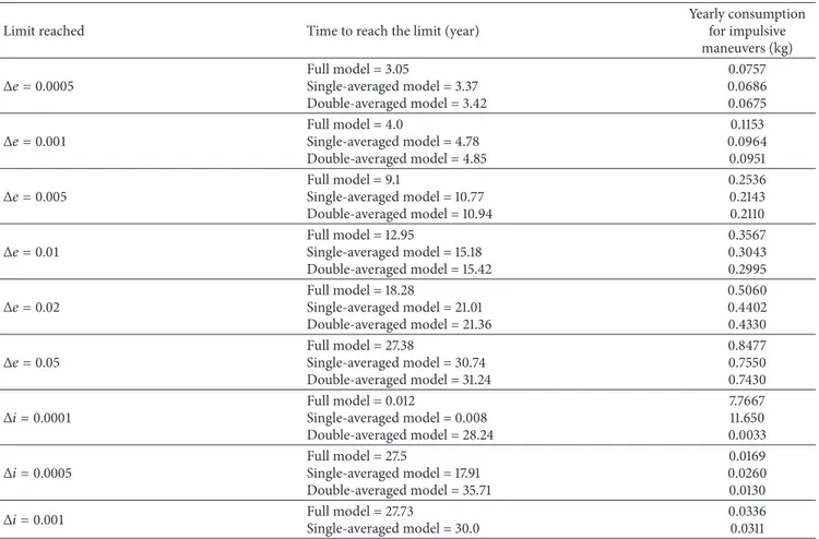
Table 9: Times when the limits are reached and the fuel consumption per year of mission assuming the value of 0.2 for the eccentricity of the orbit of the perturbing body.

0.0757 0.0686 0.0675

0.1153 0.0964

0.0951

0.2536 0.2143 0.2110

0.3567 0.3043 0.2995

0.5060 0.4402 0.4330

0.8477 0.7550 0.7430

7.7667 11.650 0.0033

0.0169 0.0260 0.0130

Δ� = 0.001 Full model = 27.73_{Single-averaged model = 30.0} 0.0336_0.0311

is that averaged models are not good enough to predict the evolution of the eccentricity and the orbital maneuvers required by the mission for near equatorial orbits, for those values of the accuracy required in eccentricity for the mission, because there is a variation of up to 0.015 in eccentricity and an average yearly consumption of up to 0.1771 kg that are not predicted by both averaged models. his average is obtained by dividing the total fuel expenditures during the mission by the total time considered for the evolution of the orbits. So, even if the spacecrat spends more than one year without the need of a maneuver, it is still possible to compute a “yearly average consumption.”

Table 5 shows the times, in years, when the limits of eccentricity are reached for each situation, as well as the estimated fuel consumption per year of mission for the several limits considered for the eccentricity and for the values of the eccentricity of the primaries.

he fuel consumptions are not too large, going from 0.0101 to 0.1771 kg per year. It is also noted that there is a strong dependence of the fuel consumption on the eccentricity of the primaries, in the order of ive times, when comparing the circular case to the case with eccentricity 0.2, for the same limits in the eccentricity variations. In the worst case considered here, with eccentricity of primaries of 0.2, the times for performing an orbital maneuver goes from 4.76

years, if the limit used for the variation of eccentricity is

Δ� = 0.0005, to 26.08 years, if the limit used for the variation

of eccentricity isΔ� = 0.01.

3.3. Near Critical Inclination Orbits. Figure 4 shows the evolution of the eccentricity and inclination, respectively, as a function of time when using the three models for the case of near critical orbits (�₀ = 39∘ ∼ 0.6803radians). In these igures, Figures4(a),4(b), and4(c)also show the results of the cases of the full elliptic restricted problem and the single-and double-averaged models, respectively. he eccentricity of the perturbing body (��) is shown in color codes: 0.0 (red), 0.1 (green), and 0.2 (blue). Regarding the full elliptic restricted three-body problem,Figure 4(a), the results show that the inclination reaches the irst limit of 0.0001 rad at 0.012 years, while the eccentricity reached several limits up to 0.02 in 28 years for the circular case for the perturbing body. It is also interesting to note that, when the eccentricity increases, there is a decrease in the inclination. By focusing on the value of the eccentricity of the perturbing body, we can see that the inclination remains close to the initial value all the time.

(13)

sufer signiicant changes with the increase in��. In the two models, the times for reaching each eccentricity limit are very close. As an example, the eccentricity 0.02 was reached in approximately 30 years in both cases. he same does not occur when the study of the inclination is made, because it reaches its limits in diferent times for each model.

he evolutions of the orbits also show another interesting feature of the averaged models. Opposite to what happens for the eccentricity, when the inclination is studied, the averaged models predict variations that are stronger than the ones observed in the real restricted three-body problem. It means that averaged models will predict orbital maneuvers and so will fuel consumption, in situations where they are really not required. Still, regarding the orbital evolution predicted by the three models, the results shown here evidence some diferences. he decrease in the eccentricity shown by the full model for the case where the eccentricity of the primaries is 0.2 is not predicted by both averaged models. he dependence of the results on the eccentricity of the primaries is much stronger when considering the elliptical restricted three-body case than when it is predicted by the averaged models, where the evolutions are similar to each other in all cases studied. Both averaged models are very similar to each other regarding predictions for the eccentricity, but they have diferences from each other for the evolution of the inclination.

Considering the limits of eccentricity and inclinations reached during the integration period, it is clear that it is necessary to perform orbital maneuvers in most of the cases.Table 6shows the times, in years, when these limits are reached for each situation, as well as the estimated fuel consumption per year of the mission for the several limits considered for the eccentricity and inclination and for diferent values of the eccentricity of the primaries.

Limits up to 0.01 in eccentricity are reached for all the models. he value 0.02 was never reached. Diferences in the prediction of the times for the maneuvers and the average yearly fuel consumption to correct eccentricities are of the order of 10%, so not too large. Regarding the inclination, for the circular case only, the limitΔ� = 0.0001was reached by the three models but the diferences in the times of the maneuver and the average yearly fuel consumption are very large among the models, with the elliptical restricted problem requiring much more fuel. When the perturbing body is not in a circular orbit, the full model takes more time to reach the limits of the eccentricity, so the averaged models predict earlier times for the maneuvers, so more yearly fuel consumption occurs when compared to the real cases. Some larger limits for the eccentricity are not reached by the full model. For the inclination, the full model predicted again higher fuel consumptions and faster orbital maneuvers than did the averaged models, so those models under evaluate the fuel consumption to correct the inclination. It is cheaper to keep lower values of the limits for the eccentricity, because the velocity of the increase in the eccentricity gets higher with the eccentricity. So, it is better to perform the maneuvers earlier, not allowing the eccentricity to grow too much. For the inclination, those costs alternate from one limit to the other.

So, the general conclusion is that averaged models are also not good enough to predict the evolution of the eccentricity and inclination also in this region of near critical inclination orbits because there are considerable diferences in the prediction of the full model and both averaged models.

3.4. High Inclined Orbits. Figures5and6show the temporal evolutions of the eccentricity and inclination, respectively, for the case of high inclined orbits, considered here to have

�0 = 80∘(∼1.3955 radians). he same representations for the

models given inFigure 4are used here.

InFigure 5, only the results of the evolution of the eccen-tricity when considering the full elliptic restricted three-body problem are showed, because similar results have been obtained for the single- and double-averaged models. his similarity is an expected result of initial inclinations above the critical value (see Domingos et al. [17]). he eccentricity oscillates with large amplitude, reaching the maximum limit of 0.06 (a variation of 0.05 from the initial value 0.01) near the time 32.5 years, while the inclination reaches only the smaller values of the limit of variation (<10−3rad) during the integration time. We note that, for the present case of

�0 = 80∘, all the limits of eccentricity are reached when

using the full problem and both averaged models, so it is necessary to perform orbital maneuvers in all the situations. Considering the inclinations, seeFigure 6, the three limits of inclination are only reached for �� = 0.2. he single-averaged model predicts earlier maneuvers than the full model does, so it overestimates the fuel consumption. he double-averaged model follows the full model better in this topic. he eccentricity of the primaries always increases the perturbations, so it also increases the average yearly fuel consumption. Tables5to9show the times when the limits are reached for each situation, as well as the estimated fuel consumption per year of mission for the several limits considered for the eccentricity and inclination for the values of 0.0, 0.1, and 0.2 for the eccentricity of the primaries.

To correct the eccentricity, the times predicted by the three models are very similar, which generates very close fuel consumption estimations. here is a strong relation between the average yearly consumption and the limits imposed on the variation in eccentricity. he cost using the limitΔ� = 0.05 is ten times more than the cost when using the limitΔ� =

0.0005. So, the more frequent the maneuvers are performed

the lower the annual cost is. Again, this is a consequence of the increase in the speed of the variation of the eccentricity with respect to the initial eccentricity. When considering the corrections in the inclination, the opposite occurs, so allowing larger limits reduces the total cost of the maneuvers per year of mission.

(14)

0 1.3940 1.3945 1.3950 1.3955 1.3960

i

(rad)

5 10 15 20 25 30 35 Time (year)

(a)

1.3940 1.3945 1.3950 1.3955 1.3960

i

(rad)

0 5 10 15 20 25 30 35 Time (year)

(b)

1.3940 1.3945 1.3950 1.3955 1.3960

i

(rad)

0 5 10 15 20 25 30 35 Time (year)

(c)

Figure 6: Evolution of the inclination as a function of time for the case�₀ = 80∘(∼1.3955 radians). In (a), the results are for the full elliptic restricted three-body problem. (b) is for the single-averaged model and (c) is for the double-averaged model. he eccentricity of the perturbing body (��) is shown in color codes: 0.0 (red), 0.1 (green), and 0.2 (blue). he dashed curves represent the (�,�) pair to perform orbital maneuvers, for each limit assumed for the inclination.

same previous pattern observed for the circular case occurs for the corrections in the inclination, and allowing larger limits still reduces the total cost of the maneuvers per year of mission.

he same analysis made before applies here. he only diference is that there is an increase in the diferences of the times to perform maneuvers and in the fuel consumptions, as a consequence, between the full and the averaged models, going to diferences close to 15% now. It is a consequence of the fact that the averaged models loss quality when the eccentricity of the primaries increases, as shown in detail by Domingos et al. [17].

4. Conclusions

he present paper studied the efects of the eccentricity of the orbit of a third-body that is disturbing a spacecrat orbiting the same central body. A hypothetical system considered here has the same masses and distances of the Earth-Moon system but has varied values for the eccentricity, in order to study its inluence in the station keeping consumption. he idea is studying potential systems of star-planet or planet-moon that exist outside the solar system in terms of learning the necessity and the cost of keeping a permanent basis orbiting those systems. In the solar system, the dwarf planet Haumea is also a good candidate to use the ideas shown here. Another contribution of this paper is to study the diferences of the single- and double-averaged models, both compared with the full elliptical restricted problem, in the times to require an orbital maneuver as well in the cost required. Emphasis is given on the estimation of the fuel consumption for station keeping maneuvers. Impulsive, with one or two impulses, and low thrust maneuvers, with one or two propulsion arcs, were used for a satellite with an initial mass of 1000 kg.

he main advantage of the low thrust system is the fuel economy, which is near four times smaller for the propulsion systems used here, due to the higher speciic impulse. When using two propulsion arcs, there is an extra saving near 10%.

For the near equatorial orbits, the averaged models are not good in predicting the evolution of the eccentricity and the orbital maneuvers. here is a variation of up to 0.015 in

the eccentricity and a yearly consumption of up to 0.1771 kg that occur using the full model but are not predicted by the averaged models. It is also shown that there is a strong dependence of the results on the eccentricity of the primaries, in the order of ive, in terms of the fuel consumption required by the circular case when compared to the case where the eccentricity is 0.2. his estimation was one of the goals of the paper.

For the near critical inclination orbits, an interesting feature of the averaged models is found. Opposite to what happens for the eccentricity, the averaged models predict variations that are stronger than the ones observed in the real restricted three-body problem. he diferences in the prediction of the times for the maneuvers and the yearly fuel consumption to correct eccentricities are in the order of 10%. For the high inclined orbits, the times predicted by the three models are very similar when studying the eccentricity, which generates very close fuel consumption estimates. So, the averaged models are good to make predictions in this range of orbits.

In general, it is noticed that there is a strong relation between the yearly consumption and the limits imposed on the variation in eccentricity. he cost using the limitΔ� =

0.05is ten times more than the cost when using the limit

Δ� = 0.0005, which indicates that the use of more frequent

maneuvers reduces the annual cost of station keeping. For the corrections in inclination, the opposite occurs.

Conflict of Interests

he authors declare that there is no conlict of interests regarding the publication of this paper.

Acknowledgments

(15)

from S˜ao Paulo Research Foundation (FAPESP) and the inancial support from the National Council for the Improve-ment of Higher Education (CAPES).

References

[1] D. Ragozzine and M. E. Brown, “Orbits and masses of the satel-lites of the dwarf planet Haumea (2003 EL61),”he Astronomical Journal, vol. 137, no. 6, pp. 4766–4776, 2009.

[2] W. Hohmann, Die Erreichbarkeit der Himmelskorper, Olden-bourg, Munich, Germany, 1925.

[3] R. F. Hoelker and R. Silber, “he bi-elliptic transfer between circular co-planar orbits,” Tech. Rep. 2-59, Army Ballistic Missile Agency, Redstone Arsenal, Huntsville, Ala, USA. [4] A. Shternfeld,Soviet Space Science, Basic Books, New York, NY,

USA, 1959.

[5] J. P. Marec, Transferts Optimaux Entre Orbites Elliptiques Proches, ONERA Publication no. 121, ONERA, Chˆatillon, France, 1967.

[6] D. F. Lawden, “Fundamentals of space navigation,”Journal of the British Interplanetary Society, vol. 13, pp. 87–101, 1954.

[7] D. F. Lawden, “Minimal rocket trajectories,”ARS Journal, vol. 23, no. 6, pp. 360–382, 1953.

[8] M. C. B. Biggs,he Optimization of Satellite Orbital Manoeuvres. Part I: Linearly Varying hrust Angles, he Hatield Polytechnic, Numerical Optimization Centre, Hertfordshire, UK, 1978. [9] M. C. B. Biggs,he Optimisation of Satellite Orbital Manoeuvres.

Part II: Using Pontryagin’s Maximun Principle, he Hatield Polytechnic, Numerical Optimisation Centre, Hertfordshire, UK, 1979.

[10] V. M. Gomes and A. F. B. A. Prado, “Low-thrust out-of-plane orbital station-keeping maneuvers for satellites,”Mathematical Problems in Engineering, vol. 2012, Article ID 532708, 14 pages, 2012.

[11] J. P. Marec,Optimal Space Trajectories, Elsevier, Amsterdam, he Netherlands, 1979.

[12] T. N. Edelbaum, “Minimum-impulse transfers in the near vicinity of a circular orbit,”Journal of Astronautical Sciences, vol. 14, no. 2, pp. 66–73, 1967.

[13] S. S. Fernandes and W. A. Golfetto, “Numerical and analytical study of optimal low-thrust limited-power transfers between close circular coplanar orbits,”Mathematical Problems in Engi-neering, vol. 2007, Article ID 59372, 23 pages, 2007.

[14] S. S. Fernandes and F. D. C. Carvalho, “A irst-order analytical theory for optimal low-thrust limited-power transfers between arbitrary elliptical coplanar orbits,”Mathematical Problems in Engineering, vol. 2008, Article ID 525930, 30 pages, 2008. [15] S. S. Fernandes, “Optimization of low-thrust limited-power

trajectories in a noncentral gravity ield transfers between orbits with small eccentricities,” Mathematical Problems in Engineering, vol. 2009, Article ID 503168, 35 pages, 2009. [16] R. C. Domingos, R. V. de Moraes, and A. F. B. A. Prado,

“hird-body perturbation in the case of elliptic orbits for the disturbing body,”Mathematical Problems in Engineering, vol. 2008, Article ID 763654, 14 pages, 2008.

[17] R. C. Domingos, A. F. B. A. Prado, and R. V. de Moraes, “A study of single- and double-averaged second-order models to evaluate third-body perturbation considering elliptic orbits for the perturbing body,”Mathematical Problems in Engineering, vol. 2013, Article ID 260830, 11 pages, 2013.

[18] G. E. Cook, “Luni-solar perturbations of the orbit of an earth satellite,”he Geophysical Journal, vol. 6, no. 3, pp. 271–291, 1962. [19] D. E. Smith, “he perturbation of satellite orbits by extra-terrestrial gravitation,”Planetary and Space Science, vol. 9, no. 10, pp. 659–674, 1962.

[20] C. R. H. Sol´orzano and A. F. B. A. Prado, “A comparison of averaged and full models to study the third-body perturbation,” he Scientiic World Journal, vol. 2013, Article ID 136528, 16 pages, 2013.

[21] K. E. Tsiolkovskii, “Investigation “the exploration of cosmic space by means of reaction devices”,”he Science Review, vol. 5, 1903.

(16)