Extracting a common high frequency signal from northern Quebec black spruce tree-rings with a Bayesian hierarchical model

(1)

CPD

5, 797–816, 2009

Extracting a common signal in tree-rings

J.-J. Boreux et al.

Title Page

Abstract Introduction

Conclusions References

Tables Figures

◭ ◮

Back Close

Full Screen / Esc

Printer-friendly Version

Interactive Discussion

Clim. Past Discuss., 5, 797–816, 2009 www.clim-past-discuss.net/5/797/2009/

Climate of the Past Discussions

Climate of the Past Discussionsis the access reviewed discussion forum ofClimate of the Past

Extracting a common high frequency

signal from northern Quebec black spruce

tree-rings with a Bayesian hierarchical

model

J.-J. Boreux1, P. Naveau2, O. Guin2, L. Perreault3, and J. Bernier1

1

The University of Li `ege, Arlon, Belgium

2

Laboratoire des Sciences du Climat et de l’Environnement, IPSL-CNRS, France

3

Institut de Recherche d’Hydro-Quebec, Montr ´eal, Canada

Received: 4 January 2009 – Accepted: 21 January 2009 – Published: 4 March 2009

Correspondence to: J.-J. Boreux ([email protected])

(2)

CPD

5, 797–816, 2009

J.-J. Boreux et al.

Title Page

Tables Figures

◭ ◮

Back Close

Full Screen / Esc

Abstract

Dendrochronology, the scientific dating method based on the analysis of tree-ring growth patterns, has been frequently applied in climatology. The basic premise of dendroclimatology is that tree rings can be viewed as climate proxies, i.e. rings are assumed to contain some hidden information about past climate. From a statistical 5

perspective, this extraction problem can be understood as the search of a hidden vari-able which represents the common signal within a collection of tree-ring width series. Classical average-based techniques used in dendrochronology have been, with dif-ferent degrees of success (depending on tree species, regional factors and statistical methods), applied to estimate the mean behavior of this latent variable. Still, a precise 10

quantification of uncertainties associated to the hidden variable distribution is difficult to assess. To model the error propagation throughout the extraction procedure, we propose and study a Bayesian hierarchical model that focuses on extracting an inter-annual high frequency signal. Our method is applied to black spruce(Picea mariana)

tree-rings recorded in northern Quebec and compared to a classical average-based 15

techniques used by dendrochronologists.

1 Introduction

1.1 Dendrochronology

In our changing climate, the search for accurate information about the past remains essential to understand and link past, present and future climate variations. Direct 20

(3)

CPD

5, 797–816, 2009

J.-J. Boreux et al.

Title Page

Tables Figures

◭ ◮

Back Close

Full Screen / Esc

on this topic can be found in Cook and Kairiukstis (1992). The fundamental assump-tion in dendroclimatology is that a climatic signal can be hidden into tree-ring growths. Since the pioneering work of Douglass (1936), dendrochronologists have developed various methods to extract such common signals for different species. A required step in dendrochronology, called standardization, is classically needed to transform ring-5

width series, that are non-stationary due to tree aging processes, into relative tree-ring indices with unit mean and a constant variance. This can be accomplished by dividing each measured ring width by its expected value, i.e. the growth trend is modelled as a regression function of tree ages. Then a common signal is derived by averaging the ensemble of such tree-ring indices across series for each year. Several methods exist 10

to calculate indices averages (e.g., Melvin et al., 2007). Esper et al. (2002) noticed that the low-frequency climate component can be highly sensitive to the standardiza-tion method. Recently, Nicault et al. (2008) proposed a neural network approach to remove the age effect and to estimate regional growth curve via explanatory variables such as tree age and their productivity. They developed a standardization procedure 15

to preserve long-term fluctuations.

In contrast with these past methods, our goal in this paper is neither to reconstruct a series of temperatures or precipitation, nor to propose novel regression schemes based on well-chosen explanatory variables as in Nicault et al. (2008). We prefer to focus on the problem of extracting a common inter-annual high frequency signal from 20

a given tree specie and region, without regressing on possible predictants. The main reason for such a choice is based on the intrinsic difficulties in linking tree-ring growths to specific explanatory variables and in interpreting these relationships. Depending on the tree specie under study, it is not always clear to dendrochronologists, even today, what are the precise contributions of precipitation, temperatures, soil and hydrological 25

(4)

CPD

5, 797–816, 2009

J.-J. Boreux et al.

Title Page

Tables Figures

◭ ◮

Back Close

Full Screen / Esc

common signal could be interpreted with respect to local measurements of tempera-tures, precipitation and other hydroclimatological variables, whenever such information would be available. Hence, independently of the estimation step, explanatory variables could be employed in a validation scheme.

1.2 Bayesian Hierarchical Modeling

5

Assessing uncertainties in any statistical dendrochronological procedure has to be carefully addressed. To tackle this important statistical issue, we opt to work within a Bayesian Hierarchical Modeling (BHM) framework. The main idea of BHMs is to statistically model a complex process and its relationships to observations in several simple components throughout a hierarchy of layers. BHMs handle elegantly and effi -10

ciently the uncertainty assessment of each layer by clearly identifying priors and pos-terior distributions of underlining processes. For an introduction to such models, see e.g. Gelman et al. (2003). In environmental sciences, BHM has become more and more popular during the last two decades. For example, Berliner et al. (2000) studied long-lead predictions of Pacific Sea Surface Temperatures via Bayesian Dynamic Mod-15

eling. Cooley et al. (2005) implemented a BHM to infer glacial retreats in Bolivia using lichen growths as a proxy. Cooley et al. (2007) estimated extreme precipitation return levels by combining BHM and extreme value theory. Concerning dendrochronology, Hooten and Wikle (2007) recently investigated with a BHM shifts in the spatio-temporal growth dynamics of shortleaf pine.

20

The uncertainty in BHM is spread over different layers, usually three. The base level, called thedata layer, characterizes observations, e.g. tree ring areas in our case. The second level in the hierarchy, called theprocess layer, models the latent process that drives the growth of such rings, tree-to-tree and regional variations. In this second layer, one can start incorporating temporal processes, e.g. the tree memories. The 25

third level, called theparameter layer, consists of the information concerning prior pa-rameters distributions that control the latent process.

(5)

CPD

5, 797–816, 2009

J.-J. Boreux et al.

Title Page

Tables Figures

◭ ◮

Back Close

Full Screen / Esc

paradigm allows the use of unobserved variables in a hierarchical structure, while eas-ily modeling uncertainties at each different level of this structure. In particular, expert information can be integrated via probability densities (the priors). In other words, past knowledge, even diffuse or imperfect, from scientists can be taken advantage of. More precisely, each parameter of a Bayesian hierarchical model can be viewed as a ran-5

dom variable and hence, a dialogue with dendrochronologists can be engaged to set the prior distribution of this random variable. If the expert has no prior knowledge then the distribution is set to be very wide (a diffuse prior), otherwise the uncertainty of the parameter can be reduced by using knowledge from past studies. In a following step, the incoming data (tree-ring areas here) are used to update all the parameters 10

of our model. The Bayes’ theorem provides the mathematical formula to perform this updating, i.e. to derive the posterior distributions. In summary, one can see the above Bayesian strategy as an assembly of elementary parts. Its modular character makes it possible to replace prior uncertainty knowledge (set by experts) by posterior distri-butional information, throughout the incoming data. In this sense, it is an evolutionary 15

construction.

The paper is organized as follows. Section 2 describes the data and the regional characteristics of the site under study. The details of our latent model are presented in Sect. 3. A short discussion about our application is proposed in Sect. 4. Perspectives are given in the conclusion.

20

2 Data and region of interest

To extract a common tree signal, the dendrochronologist has to make a series of impor-tant decisions about the tree species, the region of interest and the sampling procedure (e.g., George et al., 2008). Concerning the region choice, Hydro-Quebec, one of the founding agencies involved in this project, has had a strong interest in northern Que-25

(6)

CPD

5, 797–816, 2009

J.-J. Boreux et al.

Title Page

Tables Figures

◭ ◮

Back Close

Full Screen / Esc

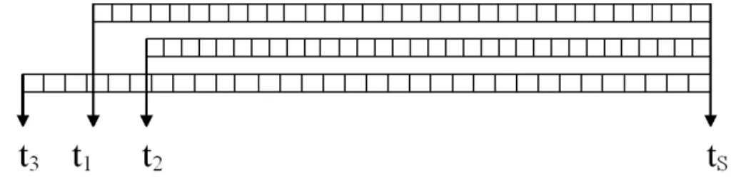
was chosen, see the red star called HM-1 in the lower panel of Fig. 1. This site has the advantages to belong to a climatic homogenous region and of being far away from most human activities. The black spruce(Picea mariana) was selected because it is a widespread specie in northern Quebec. Fifteen trees covering a period of 158 years were sampled. These trees were carefully chosen by an expert who removed singular 5

individuals (sick trees, dominated trees, etc.).

Each tree provided a ring width series from which annual growth ring areas were estimated. This transformation from ring width to ring area diminishes the geometrical effect impact, basically older trees have thiner rings. The last ring of all sampled trees, albeit missing rings, should correspond to the calendar year. Hence the youngest tree 10

determines the common period length of all trees. The diagram in Fig. 2 illustrates this phenomenon for three tree-ring series.

To illustrate the type of dendrochronological times series under study, Fig. 3 shows the temporal behavior of three ring area series, randomly chosen from fifteen trees.

The right panels represent those three ring area series. From these three right pan-15

els, it is clear that each tree has a different trend and it seems difficult to find a common hidden signal in the low frequency domain. In addition, the variability around the cubic-spline trend in the right panels seems to be stronger after 1880 for trees 1 and 2. This example illustrates the high complexity of separating tree ring areas into their individual growth component and their common hidden component in the low frequency part of 20

these signals. Different techniques (e.g. working with residuals after fitting a reference growth curve) exist to deal with this important issue. In this paper we do not address directly with issue. Instead we apply a simple non-parametric transformation to re-move trends and to work with stationary time series. This implies that we only focus on inter-annual high frequencies in tree rings. The simple non-parametric transformation 25

is defined as

Y_ts =logX_ts−logX_t₋1,s, (1)

(7)

CPD

5, 797–816, 2009

J.-J. Boreux et al.

Title Page

Tables Figures

◭ ◮

Back Close

Full Screen / Esc

S the number of trees. Transformation Eq. (1) is extensively used in finance (Gencay et al., 2002). Besides its simplicity of implementation, this log-difference has the ad-vantage of removing any smooth (i.e. polynomial) trend, see the right panels of Fig. 3. In addition the change of variability aforementioned in trees 1 and 2 is less pronounced in the right panels of Fig. 3. The drawbacks of using Eq. (1) are that, if present, the 5

low frequency part of a possible common signal has been removed and that the time unitt inY_ts does not correspond to a year anymore but to a one-year increment. The latter has to be kept in mind when interpreting our results. The former implies that our model described below will only focus on the high frequency part of a possible common signal.

10

Before closing this section we would like to emphasize that our detrending choice represented by Eq. (1) is not unique and others techniques could be used to provide stationary signals. For example, we could have worked with the residuals obtained from the cubic spline fit shown in the left panels of Fig. 3.

3 An additive latent model

15

The random variableY_tsdefined by Eq. (1) is assumed to follow an additive model with a latent variableZt

Y_ts =µ_s+λ_sZ_t+ǫ_st, (2)

witht=2, . . . , T and s=1, . . . , S, and where µ_s corresponds to the mean level of tree

s, Zt represents the hidden regional signal common to all trees and ǫst describes 20

local fluctuations of treesduring yeart. Tree-to-tree variations captured byε_stcan be due to reserves accumulated by trees and other factors that are not directly linked to environmental causes, the latter ones should be represented byZt. For each calendar

(8)

CPD

5, 797–816, 2009

J.-J. Boreux et al.

Title Page

Tables Figures

◭ ◮

Back Close

Full Screen / Esc

BHMs described in Sect. 1.2, the random variablesYts corresponds to the data layer

andZtbelongs to the process layer.

Before describing the probabilistic structure withinZ_tand ǫ_st, it is advantageous to rewrite model Eq. (2) with obvious vectorial notations

Ys =µs1+λsZ+ǫs, (3)

5

where1 is the unit vector of length T−1. Each tree s may have a temporal memory that should depend on the hydrological stress or other conditions that are particular to this tree location. Although these tree-to-tree effects can be complex, to keep the inference simple and the risk of over-parametrization low, we opt for a simple zero-mean Gaussian auto-regressive process of order one forǫ_{, i.e.} ǫ

s=φsǫ−s+Vs. The 10

notation ǫ

−s corresponds to ǫs shifted by one year, i.e. ǫ−s= εs0, εs1,· · ·, εs(T−1)

′

,

φ_s represents the auto-regressive coefficient of trees, and the random vector V_s of lengthT−1 follows a zero-mean multivariate Gaussian distribution withprecisionηs×I

whereIis the identity matrix of sizeT−1. In other words, all components of vectorVs

correspond to a standardized normal independent random noise. 15

To allow the common regional factor Zt to have a short year-to-year memory, we

assume that the latentZt can be modeled as a zero-mean Gaussian auto-regressive

process of order one, i.e.Z=ρZ₋+UwhereZ₋= Z0, Z1,· · ·, Z(T−2)

′

andUrepresents a zero-mean multivariate normal vector of lengthT−1 withprecisionτ×I.

Our full model counts 2+4S parameters, namely (ρ, τ) andθ_s₌₍_λ_s_{, µ}_s_{, φ}_s_{, η}_s_{) with} 20

s=1,2,· · ·, S. We assume that the priors distributions [ρ, τ], [θ₁_]_,_{· · ·}_{, and [}θ S] are

mutually independent. By writing the joint distribution as a product of conditional dis-tributions with a marginal distribution, the prior for (ρ, τ) can take the following form [ρ, τ]=

ρ|τ

[τ].In a classical way, we assume that the precision parameter τfollows a gamma distribution with two hyperparameters that must be fixed to reflect prior be-25

liefs. In our application, a diffuse prior is chosen by setting the two gamma parameters to zero.

The choice of the auto-regressive coefficient prior ρ|τ

(9)

CPD

5, 797–816, 2009

J.-J. Boreux et al.

Title Page

Tables Figures

◭ ◮

Back Close

Full Screen / Esc

auto-regressive coefficients have to belong to the interval [−1,1]. As Bayesian statisti-cians, we defend the idea that the underlying characteristics of the hidden processZt

should not be imposed but arise form the data via the Bayes’ rule or via prior knowl-edge. For this reason, we assume that

ρ|τ

follows a zero-mean Gaussian distribution with a precision proportional toτ. This multiplicative factor must be fixed between zero 5

and one, mainly to degrade the precision a little. In our application, we work with a diffuse prior by equaling the multiplicative factor to zero.

Concerning the prior of the random vector θ

s=(λs, µs, φs, ηs), we assume

condi-tional independence, i.e. [θ

s]=

λ_s|η_s µ_s|η_s φ_s|η_s

[η_s] where the variableη_sfollows a gamma distribution with two hyperparameters (set to zero in our application). The dis-10

tributions λs|ηs

, µs|ηs

and

φs|ηs

are assumed to be diffuse Gaussian priors in this paper. As for the auto-regressive coefficient ofZ_t, this means that the auto-regressive coefficient ofǫ_st are not a priori assumed to be in the interval [−1,1].

To compute the posteriors of the latent vector Zt and of the 2+4S parameters, we

implement the Gibbs sampler described in the Appendix. The Bayesian inference was 15

carried out with the open source R statistical software (our programs are available upon request).

4 Results and discussion

The solid line in Fig. 4 shows the estimated posterior median value of the common fac-torZtover the period 1846–2003. The shaded area corresponds to the 90% credible 20

regions (CR). Note that the value ofZ_tandλ_s are estimated up to a constant because it is always possible in Eq. (2) to multiplyZ_tby a constant and divide theλ_sby the same constant without being able to identify this multiplicative factor. In Fig. 4, we compare our BHM results with a classical technique employed by dendrochronologists. The out-put of this procedure is represented by the dashed line, a so-called tree-growth index 25

(10)

CPD

5, 797–816, 2009

J.-J. Boreux et al.

Title Page

Tables Figures

◭ ◮

Back Close

Full Screen / Esc

Kairiukstis, 1992). Up to a constant (this explains the two different scales for the y-axis), the classical tree-growth index behaves similarly toZt by staying in the CR over

a long time period. From about 1875 to 1900, there is a discrepancy betweenZ_t and the classical tree-growth index, the latter producing higher values during this period. Although fairly localized in time, this difference indicates that this classical technique 5

by not providing confidence intervals shows its limitations. Still, this comparison be-tween the two extracted signals makes us believe that our BHM approach is capable of providing meaningful outputs for dendrochronologists because they do not contradict past results and offer another statistical approach to this community of scientists.

Concerning the memory within Z_t, the posterior distribution of the autoregressive 10

coefficientρindicates a negative correlation because its 25%, 50% and 75% posterior quantiles are equal to−0.40,−0.36 and−0.32, respectively. It is interesting to note that the posterior distributions of the auto-regressive coefficient ρ belongs to the interval [−1,1], although it was not the case for their priors. In addition to CRs, our methods allow the practitioner to derive a finer analysis of her/his tree ring data. For example, an 15

analysis tree-by-tree can be undertaken. For each of the fifteen trees, Fig. 5 displays the posterior mean and 90% CRs of the parametersµs,λs and φs, respectively. The

mean posterior value of µs mostly oscillates around zero for all trees. Overall, each

tree but tree 2 appears to have a mild negative inter-annual memory, all autoregressive coefficients (but tree 2) shown in the bottom panel of Fig. 5 have aφsposterior median 20

around−0.4. The central panel clearly points out tree 1 which seem to contribute the most toZ_t.

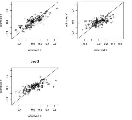
To check the quality of your estimation, Fig. 6 displays for trees 1, 2 and 3 (shown in Fig. 3), the observedYtsversus the naive estimate ˆYtsobtained by plugging our median

posterior parameter values in Eq. (2) without noise. As expected, the relationships 25

(11)

CPD

5, 797–816, 2009

J.-J. Boreux et al.

Title Page

Tables Figures

◭ ◮

Back Close

Full Screen / Esc

5 Conclusions

To summarize our findings, we have implemented a hierarchical Bayesian model to estimate a common hidden signal in high frequency component of trees. This latent signal should be viewed as a representation of the regional pressure affecting black spruce trees over our studied area in northern Quebec. The hierarchical structure pro-5

vides an elegant way to model the temporal structure associated to tree memories at the regional and tree-to-tree levels. This model attempts to quantify the contribution of a high frequency common hidden signal to each tree growth. This could help se-lecting trees with regard to a possible climatological interpretation in a reconstruction context. Compared with past approaches, our hidden signal was strongly correlated to 10

the estimate obtained with the most traditional procedure. This confirms a past method derived by dendrochronologists, while bringing the benefits of a BHM approach. As a further step in this analysis, it would be of interest to integrate low frequency in Eq. (2). One possibility is to bypass transformation Eq. (1) by making the term µ_s in Eq. (2) varying in time. For example,µ_ts could be modeled by Bayesian splines. Besides the 15

complexity of such an approach, the main difficulty is our limited sample size (fifteen trees). Ongoing field trips should provide a much larger sample of tree rings and allows us to extend our BHM procedure in future research. In this context, our present work should rather be viewed as an addition of a simple statistical procedure to the math-ematical toolbox of dendroclimatologists rather than a comprehensive study of black 20

(12)

CPD

5, 797–816, 2009

J.-J. Boreux et al.

Title Page

Tables Figures

◭ ◮

Back Close

Full Screen / Esc

Appendix A

Gibbs sampling procedure

Step 0. Initialize the vector Z|ρ, τ, z0 of length T from multivariate normal distribution

with meanz0B0and varianceτ−

1

BBT where

5

Bt₀≡hρ, ρ2,· · ·, ρTi andB=



     

1 0 0 · · ·0

ρ 1 0 · · ·0

ρ2 ρ 1 · · ·0 ..

. ... ... ... ...

ρT ρT−1· · · ρ 1



     

Step 1. Draw the precision τ|z, z0, ρ from a gamma distribution with parameters

a + T+21 and (b + 1 2

T P

t=1

z_t−ρz_t₋1

2

)−1 where a and b are prior parameters (e.g.

a=b=0) 10

Step 2. Draw the correlation coefficient ρ|z, z0, τ from a normal distribution with

mean

kρmρ+

T P

t=1

zt−1zt

kρ+

T P

t=1

z_t2₋₁

and precision

τ

k_ρ+

T P

t=1

z2_t₋₁ −1/2

wherek_ρ and m_ρ are prior

parameters (e.g.k_ρ=m_ρ=0)

Step 3.Fors=1,2,· · ·, S. 15

Step 3.1. Let ψs represent µs, λs or ϕ. Draw ψs|ys,z, z0, y0s from a normal

distribution with meankψmψ+fTsgs

kψ+gTsgs

and correlation [kψ+gTsgsηs]−

1/2

wherekψ etmψ are

(13)

CPD

5, 797–816, 2009

J.-J. Boreux et al.

Title Page

Tables Figures

◭ ◮

Back Close

Full Screen / Esc

f_s etg_sdepend on handling parameters.

Step 3.2. Draw precision η_s|µ_s, λ_s, ϕ_s,y_s,z, z0, y0s from a gamma distribution

with parametersc+T+₂3 and [d +0.5v′v]−1 where cand d are prior parameters (e.g.

c=d=0) 5

Step 4. Draw vector U|τ, η_s,L_s,R_s from a multivariate normal distribution with meanωand covarianceΩ−1and setz=z0B0+Bu. The meanωand matrixΩ

−1

relate vectorLand matrixRwhich depend on previous parameters.

10

Step 5.Return to step 1

Acknowledgements. This study is founded by the Hydro-Quebec, the CRSNG and OURANOS. The authors would like to thank Joel Guiot and Delphine Grancher for interesting discussions about the statistical aspects of dendrochronology, Yves B ´egin (INRS-ETE) and his colleagues for their data and their scientific expertise and James Merleau for his helpful suggestions. The 15

ANR Escarcel and AssimilEx projects and the MAIF foundation are also acknowledged by Philippe Naveau and Oph ´elie Guin. Finally, this paper is dedicated to the memory of Do-minique Joly.

20

(14)

CPD

5, 797–816, 2009

J.-J. Boreux et al.

Title Page

Tables Figures

◭ ◮

Back Close

Full Screen / Esc

References

Berliner L., Wikle, C., and Cressie, N.: Long-lead prediction of Pacific SSTs via Bayesian Dynamic Modeling, J. Climate, 13, 3953–3968, 2000. 800

Cooley, D., Naveau, P., Jomelli, V., Rababtel, A., and Grancher, D.: A bayesian hierarchical extreme value model for lichenometry, Environmetrics, 16, 1–20, 2005. 800

5

Cooley, D., Nychka, D., and Naveau, P.: Bayesian spatial modeling of extreme precipitation return levels, J. Am. Stat. Assoc., 102(479), 824–840, 2007. 800

Cook, E. R. and Kairiukstis, A.: Methods of dendrochronology, Kluwer Academic Publishers, 1992. 799, 805

Douglass, A. E.: Climatic cycles and tree-growth, Carnegie Institution of Washington publica-10

tion, 289, vol. 3, 1936. 799

Esper J., Cook, E. R., and Schweingruber, F. H.: Low-Frequency Signals in Long Tree-Ring Chronologies for Reconstructing Past Temperature Variability, Science, 295, 2250–2254, 2002. 799

Gencay, R., Selcuk, F., and Whitcher, B.: An Introduction to Wavelets and Other Filtering Meth-15

ods in Finance and Economics, Academic Press, San Diego, 2002. 803

Gelman, A., Carlin, J., Stern, H., and Rubin, D.: Bayesian Data Analysis, 2nd ed. Chapman andHall, 2003. 800

George, S., Meko, D. M., and Evans M. E.: Regional tree growth and inferred summer climate in the Winnipeg River basin, Canada, since AD 1783, Quat. Res., 70, 158–172, 2008. 801 20

Gelman, A.: Inference and monitoring convergence, in: Gilks, W. R., Richarson, S., and Spiegelhalter, D. J., Markov Chain Monte Carlo in Practice, Chapman and Hall, 1996. Hooten, M. B. and Wikle, C. K.: Shifts in the spatio-temporal growth dynamics of shortleaf pine,

Environmental and Ecological Statistics, 14, 3, 2007. 800

Nicault, A., Guiot, J., Edouard, J.-L., and Brewer, S.: Preserving long-term fluctuations in stan-25

dardisation of tree-ring series by Adaptive Regional Growth Curve (ARGC) Dendrochronolo-gia, submitted, 2008. 799

Melvin, T. M., Briffa, K. R., Nicolussi, K., and Grabner, M.: Time-varying-response smoothing,

(15)

CPD

5, 797–816, 2009

J.-J. Boreux et al.

Title Page

Tables Figures

◭ ◮

Back Close

Full Screen / Esc

+,%! +,%!

(16)

CPD

5, 797–816, 2009

J.-J. Boreux et al.

Title Page

Tables Figures

◭ ◮

Back Close

Full Screen / Esc

Fig. 2. This diagram indicates the temporal alignment applied to three generic tree-ring time

series. The timet_S corresponds to the youngest ring andt₁,t₂andt₃represents the age of

(17)

CPD

5, 797–816, 2009

J.-J. Boreux et al.

Title Page

Tables Figures

◭ ◮

Back Close

Full Screen / Esc

Interactive Discussion Tree ring area

tree 1

50

150

250

350

tree 2

0

50

100

150

200

250

300

year

tree 3

60

100

140

180

1850 1900 1950 2000

Tansformed tree ring area

tree 1

!

0.6

!

0.2

0.6

tree 2

!

0.4

!

0.2

0.0

0.2

0.4

0.6

year

tree 3

!

0.4

0.0

0.2

0.4

1850 1900 1950 2000

Fig. 3.Temporal behavior of three ring area time series (randomly chosen from a set of fifteen trees) over the period 1846–2003. The left panels correspond to the measured tree ring areas

with a fitted cubic spline trend. The right panels indicate the log difference of the same ring

(18)

CPD

5, 797–816, 2009

J.-J. Boreux et al.

Title Page

Tables Figures

◭ ◮

Back Close

Full Screen / Esc

1850 1900 1950 2000

!

0.4

!

0.2

0.0

0.2

0.4

year

extracted signal

year

extracted signal

0.6

0.8

1.0

1.2

1.4

1.6

Fig. 4. The solid line corresponds to the estimated posterior median value of the common

signalZ_t from Eq. (2) over the period 1846–2003. The shaded area corresponds to the 90%

(19)

CPD

5, 797–816, 2009

J.-J. Boreux et al.

Title Page

Tables Figures

◭ ◮

Back Close

Full Screen / Esc

● ●

●

● ●

µµ

−

0.01

0.03

●

● ●

●

● ●

●

● ●

λλ

0.6

0.8

1.0

1.2

● ●

●

● ●

●

● ●

●

● ●

●

● ●

●

tree label

ΦΦ

−

0.6

−

0.4

−

0.2

0.0

1 2 3 4 5 6 7 8 9 10 11 12 13 14 15

(20)

CPD

5, 797–816, 2009

J.-J. Boreux et al.

Title Page Abstract Introduction Conclusions References Tables Figures ◭ ◮ ◭ ◮ Back Close

Full Screen / Esc

Printer-friendly Version Interactive Discussion ● ● ● ● ● ● ● ● ● ● ● ● ● ● ● ● ● ● ● ● ● ● ● ● ● ● ● ● ● ● ● ● ● ● ● ● ● ● ● ●● ● ● ● ● ● ● ● ● ● ● ● ● ● ● ● ● ● ● ● ● ● ● ● ● ● ● ● ● ● ● ● ● ● ● ● ● ● ● ● ● ● ● ● ● ● ● ● ● ● ● ● ● ● ● ● ● ● ● ● ●●● ● ● ● ● ● ● ● ● ● ● ● ● ● ● ● ● ● ● ● ● ● ● ● ● ● ● ● ● ● ● ● ● ● ● ● ● ● ● ● ● ● ● ● ● ● _● ● ● ● ● ● ● ● ● ● ● ●

−0.4 0.0 0.2 0.4 0.6

− 0.4 0.0 0.4 tree 1 observed Y estimated Y ● ● ● ● ● ●● ● ● ● ● ● ● ● ● ● ● ● ● ● ● ● ● ● ● ● ●● ● ● ● ● ● ● ● ● ● ● ● ● ● ● ● ● ● ● ● ● ● ● ● ● ● ● ● ● ● ● ● ● ● ● ● ● ● ● ● ● ● ● ● ● ● ● ● ● ● ● ● ● ● ● ● ● ● ● ● ● ● ● ● ● ● ● ● ● ● ● ● ● ●● ● ● ● ● ● ● ● ● ● ● ● ● ● ● ● ● ● ● ● ● ● ● ● ● ● ● ● ● ● ● ● ● ● ● ● ● ● ● ● ● ● ● ● ● ● ● ● ● ● ● ● ● ● ● ● ● ● ●

−0.4 0.0 0.2 0.4 0.6

− 0.4 0.0 0.4 tree 2 observed Y estimated Y ● ● ● ● ● ● _● ● ● ● ● ● ● ● ● ● ● ● ● ● ● ● ● ● ● ● ● ● ● ● ● ● ● ● ● ● ● ● ● ● ● ● ● ● ● ● ● ● ● ● ● ● ● ● ● ● ● ● ● ● ● ● ● ● ● ● ● ● ● ● ● ● ● ● ● ● ● ● ● ● ● ● ● ● ● ● ● ● ● ● ● ● ● ● ● ● ● ● ● ● ● ●● ● ● ● ● ● ● ● ● ● ● ● ● ● ● ● ● ● ● ● ● ● ● ● ● ● ● ● ● ● ● ● ● ● _● ● ● _● ● ● ● ● ● ● ● ● ● ● ● ● ● ● ● ● ● ● ● ● ●

−0.4 0.0 0.2 0.4 0.6

− 0.4 0.0 0.4 tree 3 observed Y estimated Y

Fig. 6. For each of the three randomly chosen trees described in Fig. 3, the observed Y_ts