A Hierarchical Bayesian Model to Quantify
Uncertainty of Stream Water Temperature
Forecasts
Guillaume Bal1,2*, Etienne Rivot3, Jean-Luc Baglinie`re1, Jonathan White2, Etienne Pre´vost4,5
1.INRA, UMR 0985 ESE Ecologie et Sante´ des Ecosyste`mes, Rennes, France,2.Marine Institute, Oranmore, Ireland,3.Agrocampus Ouest, UMR 0985 ESE Ecologie et Sante´ des Ecosyste`mes, Rennes, France,4.INRA, UMR 1224 Ecobiop Ecologie Comportementale et Biologie des Populations de Poissons, Saint Pe´e sur Nivelle, France,5.Universite´ de Pau et des Pays de l9Adour, UMR 1224 Ecobiop Ecologie Comportementale et Biologie des Populations de Poissons, Anglet, France
Abstract
Providing generic and cost effective modelling approaches to reconstruct and forecast freshwater temperature using predictors as air temperature and water discharge is a prerequisite to understanding ecological processes underlying the impact of water temperature and of global warming on continental aquatic ecosystems. Using air temperature as a simple linear predictor of water temperature can lead to significant bias in forecasts as it does not disentangle seasonality and long term trends in the signal. Here, we develop an alternative approach based on hierarchical Bayesian statistical time series modelling of water temperature, air temperature and water discharge using seasonal sinusoidal periodic signals and time varying means and amplitudes. Fitting and forecasting performances of this approach are compared with that of simple linear regression between water and air temperatures using i) an emotive simulated example, ii) application to three French coastal streams with contrasting bio-geographical conditions and sizes. The time series modelling approach better fit data and does not exhibit forecasting bias in long term trends contrary to the linear regression. This new model also allows for more accurate forecasts of water temperature than linear regression together with a fair assessment of the uncertainty around forecasting. Warming of water temperature forecast by our hierarchical Bayesian model was slower and more uncertain than that expected with the classical regression approach. These new forecasts are in a form that is readily usable in further ecological analyses and will allow weighting of outcomes from different scenarios to manage climate change impacts on freshwater wildlife.
OPEN ACCESS
Citation:Bal G, Rivot E, Baglinie`re J-L, White J, Pre´vost E (2014) A Hierarchical Bayesian Model to Quantify Uncertainty of Stream Water Temperature Forecasts. PLoS ONE 9(12): e115659. doi:10. 1371/journal.pone.0115659
Editor:Brian R. MacKenzie, Technical University of Denmark, Denmark
Received:August 21, 2013
Accepted:November 26, 2014
Published:December 26, 2014
Copyright:ß2014 Bal et al. This is an open-access article distributed under the terms of the
Creative Commons Attribution License, which permits unrestricted use, distribution, and repro-duction in any medium, provided the original author and source are credited.
Funding:This research was performed while Dr. Guillaume Bal was a Ph.D. student sponsored by the French Ministry of Education and Research. A grant from the French Ministry of Ecology and Sustainable Development ‘Programme GICC2: Gestion et Impact du Changement Climatique’ also supported this study. The funders had no role in study design, data collection and analysis, decision to publish, or preparation of the manuscript.
Introduction
Climate change [1,2] is impacting the physiology, phenology and distributions of organisms worldwide resulting in changing communities structure [3,4]; stream ecosystems are no exception [5] with climatic changes affecting both water temperatures and discharge, key factors in the functioning of freshwater
ecosystems [6,7,8]. In particular, water temperature is of primary importance for ectothermic organisms having limited ability to adapt their spatial distributions owing their dependence on river networks and habitat fragmentation [9]. For instance, changes in water temperature affects the growth of cold water fish such as salmonids [10,11,12] and may disrupt their life histories and population dynamics [13,14,15]. Such changes may result in modifications of the
distributions [16,17,18] and ranges [19,20,21] of native species, while invasive species could be favoured [22,23,24]. This in turn can alter the structure and functioning of ecosystems, food web architecture, dynamics and energy budgets [24,25].
Long and continuous historical water temperature time series are required to assess how fluctuations of water temperature have affected the functioning of aquatic ecosystems, while forecast scenarios are prerequisite to evaluate possible impacts of future global warming. Freshwater water temperature time series are however, comparatively rare, shorter, and more prone to errors than time series of air temperature. In addition stream water temperature is rarely available as an output of climate change models. Providing tools to reconstruct and generate time series scenarios of water temperature based on commonly available
predictors, such as air temperature and/or water discharge [26,27,28], is thus a key issue.
Both mechanistic and statistical modelling approaches have been developed to predict water temperature [7]. Mechanistic models based on energy budgets are data-intensive, requiring site-specific and often costly data such as meteorological variables other than air temperature, topography and stream bed information [29,30,31,32]. They provide fine scale estimates of the water temperature but are difficult to use for forecasting stream temperatures on wider geographical scales because of the amount of data needed.
Simple linear regression models between air and water temperatures have been one of the most used approaches to infer water temperature [39,40,41,42,43]. Because of their simplicity and low data requirement, these simple approaches are quite popular among freshwater ecologist to reconstruct and/or forecast stream temperature time series[44,45,46]. However, simple regression models suffer from methodological caveats that have received little attention in the literature. Both air and water temperature signals show seasonal fluctuations with maximum amplitudes of approximately 15 to 25
˚
C. The synchrony between the two signals due to seasonal fluctuations will thus result in strong positive correlations between pairwise records of water and air temperatures that could hide joint patterns of the evolution of air and water temperatures over longer time scales [34,35,40,47]. Simple models based on this positive correlation could thus lead to biased water temperature forecasts or to underestimation of the associated uncertainty.In this paper, we develop a generic statistical approach to forecast water temperature from air temperature and water discharge time series that allows the components of the correlation owing to seasonality to be separated from those owing to longer term fluctuations or trends. The approach is developed in a fully hierarchical Bayesian framework that provides a probabilistic rationale to propagate and quantify uncertainty around inferences and predictions [48]. To demonstrate the potential of our approach we compared its performance to that of simple linear regression over a short time scale on i) a simulated example, and ii) time series of air temperatures, water discharge and water temperatures from three French coastal streams of contrasting size and bio-geography.
Material & Methods
1. Modelling and forecasting water temperature
Limits of simple regression models: a simulated illustrative example
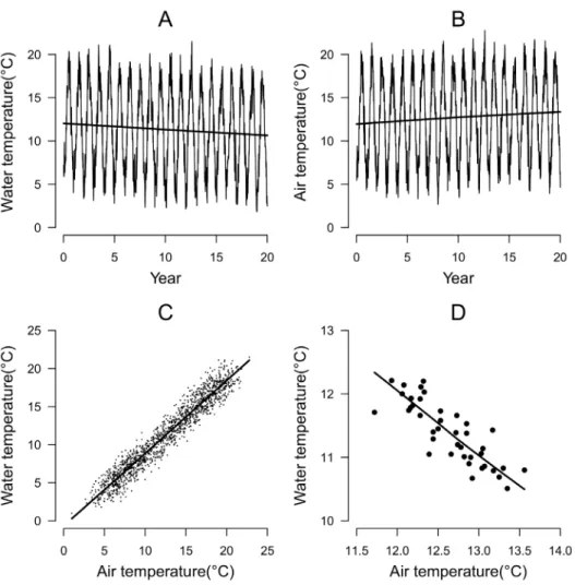
To illustrate the potential caveats of simple regression models between water and air temperature, we simulated water and air temperature time series exhibiting characteristic seasonal fluctuations and weak but opposite long term time trends (Fig. 1). Daily water temperatures were simulated using a sinusoidal function with an annual periodicity and amplitude of 13
˚
C, plus a negative trend in the annual mean of 20.5˚
C over 20 years starting from an original mean of 12˚
C. The time series of air temperature was simulated with the same periodicity and amplitude but with an increasing trend of +0.5˚
C over the 20 years. Both time series wereThis simulated example illustrates that relying on only the strength of the short term correlation to forecast water temperature could be inappropriate as it may lead to erroneous conclusions regarding the long term evolution of water temperature. By contrast, correlations calculated over a longer time period will only pick up the associations between signals with longer periodicity. Neither of these approaches however, allows both the seasonal and longer term trends to be simultaneously captured. Moreover, simple regressions between air and water temperatures do not account for the influences of other covariates such as water discharge. A more consistent statistical approach should account for both seasonality and long term trends in the climatic time series and the potential effect of water discharge as a covariate.
Fig. 1. Linear regressions between pairwise records of air temperatures and water temperatures at small time scale (moving average over 5 days; panel C) and long time scale (moving average over 6 months; panel D).
Separating seasonality from longer time trends: model M1
Model M1 is a fully Bayesian hierarchical model based on time series
decomposition according to eq (1)and is composed of three modules which are all embedded within the same hierarchical model (detailed hereafter). The first module aims at decomposing the time series of predictors (air temperature and water discharge) and response variable (water temperature) into long term trends, seasonal fluctuations and residual variability; In the second module, some relations are introduced in the hierarchical structure to characterize the
relationships between the time series of the water temperature and its predictors at different time periodicity; In the third module, these relationships are used to forecast water temperature from air temperature and water discharge.
In module (1), air temperature and log-transformed river flow time series were decomposed using eq. (1) [34], whereXy,t represents the time series of a variable
(indifferently air temperature, water temperature or (log-transformed) water discharge).
Xy,t~ayzby|sin
2p
n (tzt0)
z t ð1Þ
ayandbyare the mean and amplitude on the time windowyrespectively. A
five-day arithmetic average was used as the short time steptso n is equal to 73. A long-term window of 6 months was set for the longer time windowy.Preliminary trials have shown that averaging over five days was the best compromise between the computational performances (the computational time increases with the number of time steps) and the degree of smoothing of short term variability. Using long term windows of 6 months (instead of 1 year) maximizes the number of time step used to fit relationships ineqs. (2a)-(2b)(see hereafter).t0sets the position of the
sine signal on the time line. Preliminary analyses using parameters t0 that vary
between periods y have shown only very slight variability of t0 between periods
(not shown), and t0was therefore assumed constant in time. As residual random
terms of the three time series are known to exhibit significant positive
autocorrelation, random terms t were modelled as a first order autoregressive process with autocorrelation coefficient r and variance of the innovationss2
. Time series of random terms were modelled as mutually independent between the time series (water and air temperature, water discharge). Measurement errors were not included in the model. As observation errors were quite low when compared to the natural variability on our three case study (see Annexe 1), they were unlikely to impact on the results and have not been modelled. Priors specified for the unknown parameters(ay,by,t0,r ,s2)were all weakly informative
(Table 1).
In module (2) of the hierarchical modelM1, parameters describing the shape of
two of these four parameters(ay,by,maxy,miny), where maxy~ayzby and
min
y~ay{by are the maximum and the minimum of the signal, respectively. Here, the sine signal of water temperature (WT) was parameterized in terms of maximum maxWT
y and minimum minWTy allowing the impact of air temperature (AT) and discharge (Q) to be integrated. maxWT
y was defined as a linear function of the maximum air temperature and minimum water discharge (eq. (2a)), while
minWT
y was defined as a linear function of the minimum air temperature and maximum water discharge (eq. (2b)):
maxWT
y *Normal(mmaxWT
y ,s
2 maxWT)
withm
mawWTy ~h0zh1|max AT
y zh2|minQy
ð2aÞ
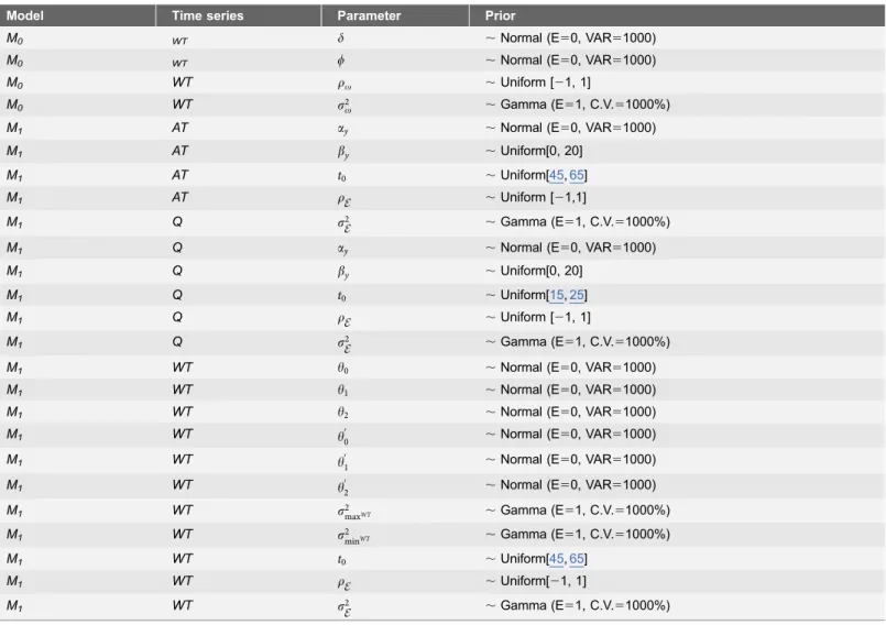
Table 1.Prior distributions assigned on parameters in modelsM0andM1.
Model Time series Parameter Prior
M0 WT d ,Normal (E50, VAR51000)
M0 WT w ,Normal (E50, VAR51000)
M0 WT rv ,Uniform [21, 1]
M0 WT s2v ,Gamma (E51, C.V.51000%)
M1 AT ay ,Normal (E50, VAR51000)
M1 AT by ,Uniform[0, 20]
M1 AT t0 ,Uniform[45,65]
M1 AT r ,Uniform [21,1]
M1 Q s2 ,Gamma (E51, C.V.51000%)
M1 Q ay ,Normal (E50, VAR51000)
M1 Q by ,Uniform[0, 20]
M1 Q t0 ,Uniform[15,25]
M1 Q r ,Uniform [21, 1]
M1 Q s2 ,Gamma (E51, C.V.51000%)
M1 WT h0 ,Normal (E50, VAR51000)
M1 WT h1 ,Normal (E50, VAR51000)
M1 WT h2 ,Normal (E50, VAR51000)
M1 WT h0
0 ,Normal (E50, VAR51000)
M1 WT h0
1 ,Normal (E50, VAR51000)
M1 WT h
0
2 ,Normal (E50, VAR51000)
M1 WT s2maxWT ,Gamma (E51, C.V.51000%)
M1 WT s2minWT ,Gamma (E51, C.V.51000%)
M1 WT t0 ,Uniform[45,65]
M1 WT r ,Uniform[21, 1]
M1 WT s2 ,Gamma (E51, C.V.51000%)
E, VAR and C.V/correspond to expectation, variance and coefficient of variation respectively.
minWT
y *Normal(mminWT
y ,s
2 minWT)
withm minWT
y ~h
0
0zh
0
1|minATy zh
0
2|maxQy
ð2bÞ
Previous analyses have shown that the best compromise between the complexity of the relationships and the quantity of deviance explained was obtained through this set of simple linear regressions. Moreover,eqs (2a)-(2b)are quite interpretable in term of environmental processes. h1 is expected to be
positive as maxWT
y series is expected to be positively correlated with the maxATy series. h1 is expected to be negative as high minimum discharge is expected to
decrease the seasonal variation of water temperature because higher minimum water discharge generally corresponds to cool temperatures in summer. h01,h
0
2are
both expected to be positive, as warmer air relates to warmer water and a high water discharge in winter tends to relate to high water temperatures because high winter flows correlate with wet and mild conditionss2
. Weakly informative prior
distributions were set for unknown parameters (h0,h1,h2,h
0 0,h 0 1,h 0 2,s 2 minWT,s
2 maxWT)
(Table 1). As stated in the above section, random terms in water temperature were modelled as a first order autoregressive process assumed to be independent from that of the air temperature and flow time series’. Weakly informative parameters were set on related parameters (Table 1). Observation errors were not modelled. Finally module (3) is a forecasting module embedded in the hierarchical model
M1 that uses the information from module (1) and (2) to forecast the water
temperature while fully propagating the uncertainty through the hierarchical structure. We denote AT9and Q9the time series’ of air temperature and water discharge from which we want to forecast water temperature WT9. Such series may be historical observations or climatic model scenarios. AT9 and Q9 are first decomposed following the model described in eq. (1) to obtain estimates of parameters (maxAT
y ,minATy ,maxQy ,minQy ). Relationships (2a)-(2b), combined with the regression parameters (h0,h1,h2,h
0 0,h 0 1,h 0 2,s 2 maxWT,s
2
minWT)are then used to
forecast parameters maxWT
y andminWTy series, which characterise the forecast sine signal of WT9. Combined with the variance of noise around this, the whole WT9
series can be forecast conditionally upon all the information conveyed by the historical series of water temperature, air temperature and water discharge and upon AT9 andQ9series. In a Bayesian framework, this is done through the posterior predictive distribution [49]of the forecast time series WT9, that
A simple linear regression model
For the purpose of comparison, a linear regression model between water and air temperatures (M0) was also implemented and fitted in a Bayesian framework
using pairwise historical records averaged over 5 days using the following equation:
WTy,t~dzQ|ATy,tzvt ð3Þ
Residual random termsvtwere modelled as a first order autoregressive process with autocorrelation coefficient rvand variance of the innovations s2
v. Non informative prior distributions were used for parameters in eq. (3) (Table 1). Posterior distributions of the parametersd,Q,s2
vand the series of air temperature
AT9were used to provide posterior predictive distributions of the forecasted time series WT9.
2. Bayesian computation
Bayesian fitting, forecasting and the derivations were implemented using Markov Chain Monte Carlo algorithms in JAGS (Just Another Gibbs Sampler) [50] through the R software [51]. Three parallel MCMC chains were run and 20,000 iterations from each were retained after an initial burn-in of 20,000 iterations. Convergence of chains was assessed using the Brooks-Gelman-Rubin diagnostic [52].
3. Posterior checking, model comparison and cross validation
The consistency between the model a posteriori and the data was assessed via posterior checking techniques [49]. If model fits, then replicated data generated under the model should look similar to observed data, i.e. data should look plausible under the posterior predictive distribution. Any systematic discrepancy coming from this ‘‘self consistency’’ check indicates potential failing of the model. Here, we employ as a discrepancy measure the x2 discrepancy statistic [49]. For each model, the x2statistic was calculated as:x2(WT,h)~X
y
X
t
(WTy,t{E(WTy,tjh))
2
) Var(WTy,tjh)
ð4Þ
where E(WTy,tjh) and Var(WTy,tjh)are respectively the expected mean and variance of the water temperature conditionally upon the parameters h. For each set of parameters (y) drawn in their joint posterior distributions, the realized discrepancies x2
(WTobsjh)computed with the observed values of water temperature were compared against the predicted discrepancies x2
(WTrepjh) computed with posterior predictive replicates of water temperature. If the model is consistent with the data, x2
(WTrepjh) should be similar tox2
(WTobsjh). The Bayesianp-value was calculated as the probability thatx2
estimated over the posterior sample ofh.Ap-value near 0.5 indicates consistency between model and data, whereas a very high (0.95) or low (0.05) p-value provides serious warning.
The Deviance Information Criterion (DIC) [53] was also used to compare the goodness of fit of modelsM0 andM1. As with the Akaike Information Criterion,
DIC combines a measure of the goodness of fit penalized by a measure of the model complexity. The smaller the DIC, the more a model is supported by data.
The predictive performances were compared through cross-validation analyses. A cross-validation was implemented using the first two thirds of the available time series to fit the model and make forecasting on the last third. These were subsequently compared against known temperatures. Differences between the observed and predicted water temperatures were quantified using the root mean square error (RMSE) [37,41,54].
4. Application
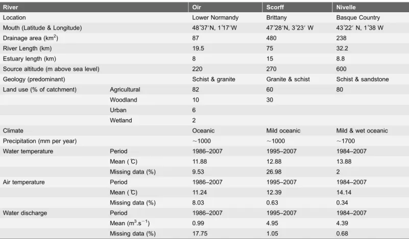
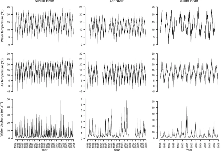
Our approach was applied to i) the illustrative simulated time series of air and water temperature and ii) time series of water temperature, air temperature and water discharge from three coastal streams of the French Environmental Research Observatory for Small Coastal Streams (ERO SCT;Fig. 2which benefits from long term monitoring of environmental parameters and fish populations; the Oir River [55,56], the Scorff River [57] and the Nivelle River [58]. The main characteristics of rivers and associated data are summarized in Table 2and Fig. 3. More details about the Rivers are provided in Annexe 1 and data used in this study can be made available by contacting staff members of the ERO SCT (https://www6.inra. fr/ore-pfc).
5. Forecasting scenarios
For the illustrative example based on simulated data, models M0 and M1 were
applied to forecast water temperatures, with a simplified version of model M1
(eq.1 to 3) using air temperature as the only predictor of water temperature. Water temperature was forecast based on a 50 years extension of air temperature simulated with a linear increment in the annual mean resulting in a warming of
+3.2
˚
C (corresponding to the maximum air temperature increments supported bythe IPCC (2007) [1].
The three simulated scenarios, extended from the coastal stream examples, also consisted of 50 years of air and water temperature and discharge data. Air temperatures were simulated with the same+3.2
˚
C linear increment in the annualmean. To allow for comparisons between outputs of models M0 andM1, the
Results
First, we compare the forecasts of water temperature provided by the models M0
and M1with the simple simulated example. Then, we compare the quality of fit,
the internal consistencies (posterior checking) and the forecasting performances (cross validation) of the two models when applied on the three coastal streams. Lastly, we provide some key features of the results of the model M1.
1. Simulated illustrative example
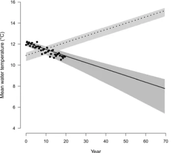
Fig. 4 highlights that the two modelling approaches lead to different forecasts of water temperature. Simulations from M0 are based on the positive correlation
between air and water temperatures owing to their synchronous seasonal
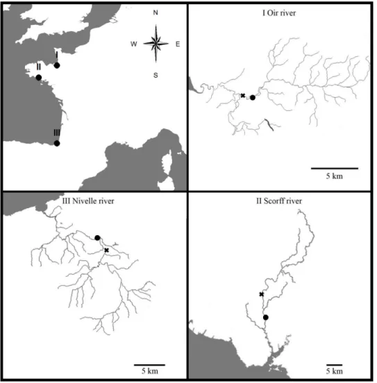
fluctuations, which logically leads to forecast an increase in the water temperature. Fig. 2. Watersheds of the three case study rivers. x: hydrometric station;
N
: water temperature measurement stations.By contrast,M1captures the difference in long term trends in air temperature and
water temperature and hence produces a decreasing trend in water temperature, which is more consistent with the observed patterns in the historical time series. The 95% credibility envelope around the forecast produced by M1 is also wider
than that produced by M0.
2. Applications to coastal streams data
Posterior checking, model comparison and cross validation
Overall, when applied to the data from the three coastal streams, the model M1
produces similar results toM0in term of internal consistency and outperformed it
in terms quality of fit and predictive performance.
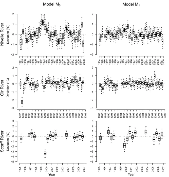
For each of the three coastal streams, discrepancies between observed and fitted means calculated on 6 months intervals are globally smaller for modelM1than for
model M0 (Fig. 5). This value appeared close to 0.5 in case of both models
indicating equivalent posterior consistency with data. It is worth noting that the simple regression approachM0was not able to capture the variability in the data
for the years 1991, 1992 and 1993 for the Nivelle River, 1987 for the Oir River and 1999 for the Scorff River.
Table 2.Study rivers characteristics and summary of data sets.
River Oir Scorff Nivelle
Location Lower Normandy Brittany Basque Country
Mouth (Latitude & Longitude) 48˚379N, 1˚179W 47˚289N, 3˚239W 43˚229N, 1˚38 W
Drainage area (km2) 87 480 238
River Length (km) 19.5 75 32.2
Estuary length (km) 8 15 8.8
Source altitude (m above sea level) 220 270 600
Geology (predominant) Schist & granite Granite & schist Schist & sandstone
Land use (% of catchment) Agricultural 82 60 80
Woodland 10 30
Urban 6
Wetland 2
Climate Oceanic Mild oceanic Mild & wet oceanic
Precipitation (mm per year) ,1000 ,1000 ,1700
Water temperature Period 1986–2007 1995–2007 1984–2007
Mean (˚C) 11.88 12.88 13.88
Missing data (%) 9.53 26.98 2
Air temperature Period 1986–2007 1995–2007 1984–2007
Mean (˚C) 11.24 12.39 14.14
Missing data (%) 8.03 0.63 0.34
Water discharge Period 1986–2007 1995–2007 1984–2007
Mean (m3.s21) 0.99 4.95 4.39
Missing data (%) 17.75 1.05 0.68
x2
discrepancies and associated p-values for the two models do not reveal inconsistencies between the models and the data from the three rivers as all p -values are close to 0.5 (Table 3).
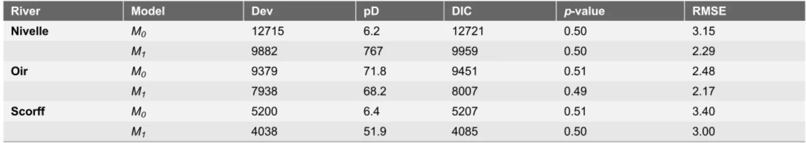
Deviance Information Criterion clearly indicates a better fit of modelM1for the
three coastal streams (Table 3). The posterior means of deviances are much greater for model M0, and differences are not counterbalanced by the higher
model complexity of modelM1. The high number of parameters estimated on the
Oir River for model M0 (pD571.8, Table 3) differs to that of the Scorff and
Nivelle Rivers (pD close to 6 in each case,Table 3) and is attributed to the higher frequency of missing air and water temperature data for the Oir River (in the Bayesian framework missing data are considered as unknown values to be estimated).
The RMSE (Table 3), used as a summary measure to quantify the predictive performances of both models, indicates better predictive performances for model
M1on the three rivers. Even when a large proportion of missing data for any one,
or for multiple time series’ could have impeded the precision in the parameter Fig. 3. Time series of the available data on the three rivers used as case studies.
estimates ineqs. (2a)-(2b), the performance of the new method was superior in its estimates than those of modelM0.See for instance air and water temperature data
in 1990, 1991, 1992 and 1994 on the Oir River together with the high proportion of missing data for water discharge between 2001 and 2004, which represented nearly half of the forecasting period.
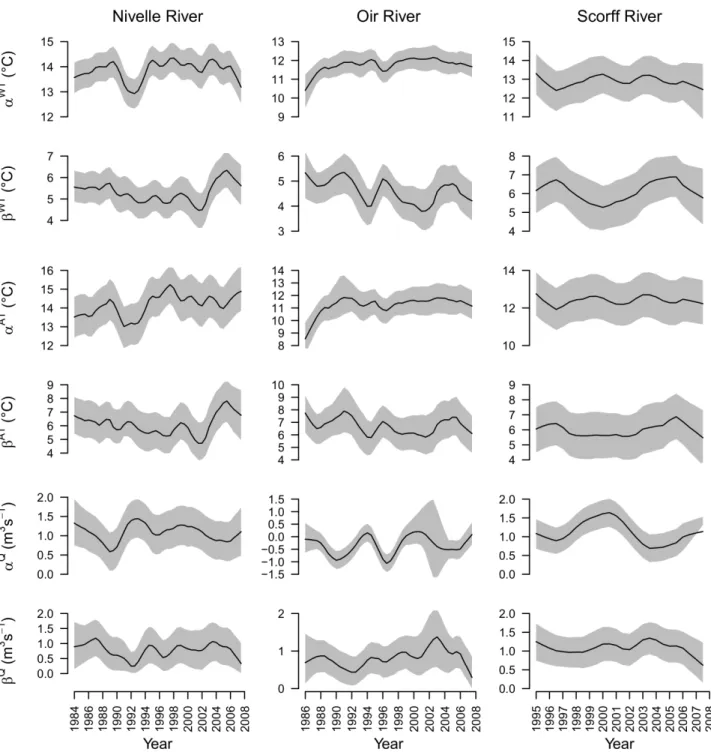
Means and amplitudes of the air temperature, water discharge and water temperature time series
Bayesian estimates of means and amplitudes (estimated for every 6 months intervals) vary between time intervals, and with the exception of increasing trends in the mean water temperature of the Oir River and air temperature of the Nivelle and Oir rivers, no other clear trend emerged. Uncertainty around estimates is quite low (Fig. 6) and slightly lower for periods with higher proportion of missing data (see for instance the period 2001–2004 for water discharge on the Oir River).
Overall mean water temperature increased from north (Oir R.) to south (Nivelle R.). Amplitudes of air temperature were close to 6
˚
C and the amplitudes of water temperature increased with river lengths and catchment areas (Scorff R..Nivelle R..Oir R.). Time series of mean water and air temperatures appear to be positively aligned, while time series of water amplitudes appeared to be positively aligned with amplitudes of air temperatures but buffered by occurrences of high mean flow (Fig. 6.).
Fig. 4. Evolution of temperatures predicted by the modelling approachesM0andM1for the simple
simulated example.Posterior means are represented by a full line for the modelM1and a dotted line for
modelM0. 95% Bayesian credibility intervals corresponds respectively to dark and light grey shaded areas for
modelsM1andM0. Points correspond to initial data.
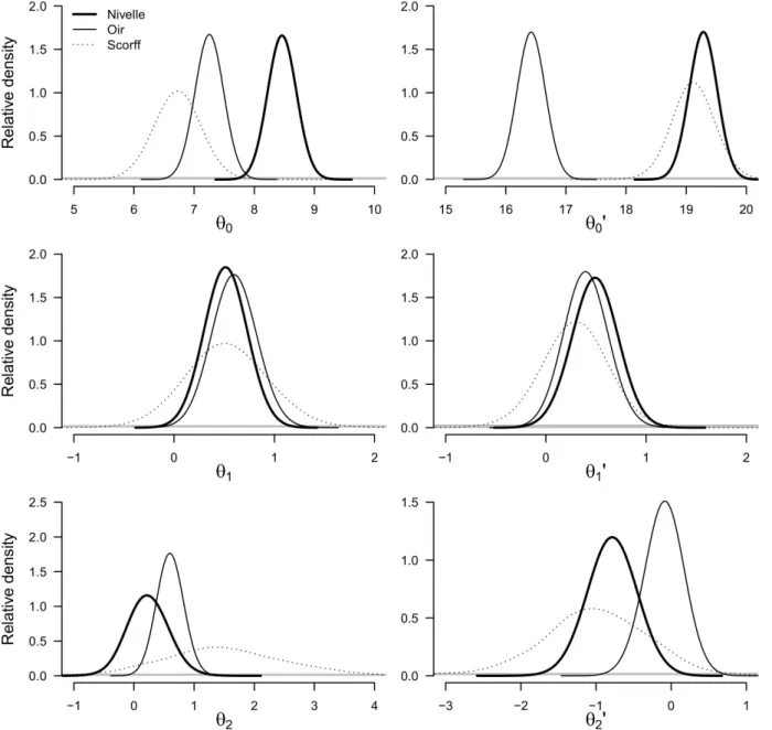
Estimates of parameters linking water temperature to air temperature and water discharge
Posterior estimates of regression parameters linking the characteristics of the water temperature sine signal to that of the air temperature and water discharge are consistent overall with our expectation (Fig. 7). Bayesian posterior distribu-tions of all parameters have only low probability to be negative, except h02.
Fig. 5. Boxplots of the differences between observed and fitted means of water temperatures by six month blocks on the three Rivers with the modelling approachesM0andM1.Only blocks with representative data were included.
Uncertainties around parameter estimates are greater for the Scorff River, for which data series are shorter (13 years) than those of the Nivelle and Oir Rivers (24 and 22 years respectively). Maximum flow nonetheless had negligible effect on minimum water temperature for the Nivelle River (posterior distribution of h2
around 0). The relationship between the time series of minimum flow and of the maximum water temperature is also weak (posterior distribution of h02 centred
around 0) (Fig. 7).
Forecasting water temperature from climatic scenarios
Based on the 50 years climatic scenarios, Bayesian forecasts of water temperature produced by both models M0 and M1exhibit clear increasing trends but the
median trends forecast by the modelling approach M1 were significantly weaker
(Fig. 8). The mean warming of stream water by the end of the 50 years forecasting period ranges from around 1.5
˚
C to 2.5˚
C according to modelM0while the threeforecast of model M1 were 0.2 to 1.5
˚
C lower.Meanwhile, the models exhibit strong differences in the uncertainty around forecasts (Fig. 8), the greater predictive performance and quality of fit of model
M1being accompanied by a greater uncertainty in the forecasted trends, with 95%
credibility intervals at least 1.4 times greater than from modelM0. The probability
that the forecast water temperatures exceeded the average temperature observed in the last ten years can be used as a synthetic metric to compare the forecasts between M0 andM1. According to model M0, the number of forecasting years
after which this probability exceeds 95% is less than 20 years. According to model
M1, this would occur latter on the three Rivers and are not forecast in case of the
Scorff River. Nonetheless, forecasting intervals are still overlapping by the end of the forecasting period (Fig. 8).
Reconstruction of missing data using model M1
Missing data are considered in Bayesian modelling as unknown variables that can be estimated directly from their posterior predictive distribution [49]. This is illustrated for the Oir River (Fig. 9) where water temperature reconstructed from Table 3.Model selection, posterior checking and predictive performance for the two modelling approaches applied to the 3 rivers.
River Model Dev pD DIC p-value RMSE
Nivelle M0 12715 6.2 12721 0.50 3.15
M1 9882 767 9959 0.50 2.29
Oir M0 9379 71.8 9451 0.51 2.48
M1 7938 68.2 8007 0.49 2.17
Scorff M0 5200 6.4 5207 0.51 3.40
M1 4038 51.9 4085 0.50 3.00
Dev: deviance posterior mean; pD: measure of the model complexity (estimated number of parameters); DIC: Deviance Information Criterion. value: p-value for the posterior checking tests; RMSE: root mean square errors used to quantify the predictive performance.
estimates are close to the observed variations of water temperatures around the underlying mean seasonal pattern, showing that estimated water temperatures are good approximation of the true water temperatures.
Fig. 6. Posterior distribution of the means (a) and amplitudes (b) characterizing the time series of water temperature (WT), air temperature (AT) and water discharge (Q) on the three rivers.Solid line: posterior medians; shaded area: 95% posterior interval.
Discussion
The effect of climate warming on river temperatures is no longer just speculative, with an observed warming up to 1
˚
C per decade [7,8,36]. Providing generic models to reconstruct and forecast water temperature series based on predictors such as air temperature and water discharge, for which historical series or predictions from scenarios of climate change are available, is a prerequisite to better understand how water temperature drives ecosystems functioning, and to Fig. 7. Posterior distributions of the parameters involved in the linear regression used to infer the time series of stream water temperatures based on time series of air temperature and discharge used as predictors.framework allowing weighting of the outcomes of different management scenarios is a cornerstone for further biological conservation [48,59,60]. The time series modelling approach (M1) developed in this paper offers a useful contribution to
these challenges.
Fig. 8. Average temperature calculated for 6 months intervals forecasted by the modelling approachesM1andM0on the three rivers over 50 years
under an air temperature warming scenario of 3.2˚C.Posterior means are represented by solid lines for the modelM1and dotted lines for modelM0. 95%
Bayesian credibility intervals correspond respectively to dark and light grey areas for modelsM1andM0respectively. Horizontal Black line: average water
temperature observed over the last ten year time series.
doi:10.1371/journal.pone.0115659.g008
Fig. 9. Observed (black line) and estimated missing water temperatures (black dotted line) using modelM1with 95% Bayesian credibility interval (grey area) on the Oir River in 2006.
The time series decomposition approach has several advantages over the linear regression modelling (M0). It can be used to reconstruct continuous time series of
discharge, air and water temperatures in the presence of missing data without additional predictors. The method proved useful in reconstructing continuous water temperature time series for three French coastal streams, even with important proportions of the records missing. The time series modelling
approach also allows disentangling seasonal periodicity from longer time trends. The illustrative simulated example demonstrated that a simple regression model between air and water temperature does not distinguish between temporal scales lead to different conclusions. Owing to the ability to separate seasonality from long term trends, the methodology based on time series modelling allows for unbiased and more accurate predictions of the water temperature.
When applied to the time series of three coastal streams, the time series modelling approach outperforms the simple linear regression model in quality of fit and predictive performances. The DIC favoured the time series modelling approach despite a higher number of parameters. For the three rivers, cross validation analysis show that the time series modelling approach has better predictive performance than the simple regression. The 50 years forecasting scenarios also shows that the simple regression approach M0provides unduly
warmer forecast of water temperature by comparison with the time series approach M1. Only the posterior checking, which does not compare the
forecasting precision of the two methods, show that the two modelling approaches had equivalent posterior consistency with data.
The time series modelling approach could be developed further. A first research direction to improve statistical modelling could consist of implementing more elaborate modelling of random variation around the mean signal. For instance, the covariance between water temperature residuals and the residuals of the predictors could be explicitly incorporated [7,33]. Observation errors could also be modelled if they are thought to be high and the information to do so is available. Furthermore, additional predictors could also be incorporated. Our time series modelling approach ignores many other factors that may play an important role in controlling water temperature, for example predictable changes in riparian vegetation were not considered in the present study although they have been shown to influence water temperature [64,65,66]. The impact of climate change on groundwater discharge and associated spatial heterogeneity of water temperatures, which are of primary importance for the survival of many cold water fish under high temperature stress [67,68] could be included in the model as well as other climate variables such as evapo-transpiration or solar radiation.
To conclude, the outputs of our model could be used to assess the past and future effects of water temperature on very specific ecological mechanisms such as the growth of juvenile salmonids [12]. More generally, water temperature scenarios are essential inputs for evaluating the effects of climate change on various broader ecological processes such as the dynamics of fish population [15,69,70] or food webs [24,25]. By virtue of the Bayesian framework proposed, river water temperature, an important and yet often unrecorded variable may be estimated and forecasted with its uncertainty fully integrated, an important issue in resource management and ecology.
Annexe 1
The Oir River flows into the estuarine part of the Se´lune River, 8 km from the Bay du Mont Saint Michel. Water temperatures were measured by Tidbit temperature data loggers (¡0.2
˚
C) daily at the Cerisel station (Fig. 2) by the National Institute of the Agronomic Research (INRA). Daily air temperatures were obtained from the meteorological station at Saint-Hilaire-du-Harcoue¨t, 14 km east of the water temperature station. Water discharge was measured just upstream of theconfluence with the Se´lune River, while data were available for 22 years (1986 to 2007), 11.8% of data were missing over the three time series.
The Scorff River flows in to the Atlantic Ocean (Fig. 2). Daily water
temperature measurements were made with Tidbit data loggers (¡0.2
˚
C) at the Moulin des Princes station by INRA. Daily air temperatures were obtained from the Lorient (Lan Bihoue) airport meteorological station, 9 km south of the water temperature station while discharge was monitored 8 km upstream. Data were available for 13 years (1995 to 2007), 9.6% data were missing for the three series.Tidbit (¡0.2
˚
C) temperature data loggers. Daily air temperatures were recorded 13 km to the north at the Biarritz airport meteorological station. Water discharge was measured at the confluence with its main tributary, the Lurgorrieta. 24 years of data were available (1984 to 2007), with 1% missing across the three time series.Acknowledgments
We thank Dr Andre´ St-Hilaire, Dr Eric J. Ward, anonymous referees and the editor of the Plos One Journal for their helpful comments on the earlier version of this manuscript. We are also grateful to the staff of the ‘‘Unite´ Expe´rimentale d9Ecologie et d9Ecotoxicologie Aquatique’’ (INRA Rennes), the ‘‘Unite´ Mixte de recherche INRA/UPPA Ecologie Comportementale et Biologie des Populations de Poissons’’ (INRA Saint-Pe´e-sur-Nivelle), the ‘‘Unite´ Expe´rimentale d9Ecologie et d9Ecotoxicologie’’ (INRA Rennes) of the ‘‘Unite´ Agroclim’’ (INRA PACA) and of Me´te´o France for providing the data used in this study.
Author Contributions
Analyzed the data: GB ER EP JLB JW. Contributed reagents/materials/analysis tools: GB ER EP JLB JW. Wrote the paper: GB ER EP JLB JW.
References
1. Intergovernmental Panel on Climate Change(2007) Climate Change 2007: The Physical. Science Basis: Intergovernmental Panel on Climate Change Fourth Assessment Report. Available athttp://www. ipcc.ch/.
2. Betts RA, Collins M, Hemming DL, Jones CD, Lowe JA, et al.(2011) When could global warming reach 4 degrees C? Philos T Roy Soc A 369: 67–84. doi: 10.1098/rsta.2010.0292
3. Walther GR, Post E, Convey P, Menzel A, Parmesan C, et al.(2002) Ecological responses to recent climate change. Nature 416: 389–395. doi: 10.1038/416389a
4. Parmesan C, Yohe G(2003) A globally coherent fingerprint of climate change impacts across natural systems. Nature 421: 37–42. doi: 10.1038/nature01286
5. Heino J, Virkkala R, Toivonen H(2009) Climate change and freshwater biodiversity: detected patterns, future trends and adaptations in northern regions. Biol Rev 84: 39–54. doi: 10.1111/j.1469-185X
6. Schindler DW(2001) The cumulative effects of climate warming and other human stresses on Canadian freshwaters in the new millennium. Can J Fish Aquat Sci 58: 18–29. doi: 10.1139/cjfas-58-1-18
7. Caissie D(2006) The thermal regime of rivers: a review. Freshwater Biol 51: 1389–1406. doi: 10.1111/ j.1365–2427.2006.01597.x
8. Ormerod SJ(2009) Climate change, river conservation and the adaptation challenge. Aquat Conserv 19: 609–613. doi: 10.1002/aqc.1062
9. Portner HO, Farrell AP(2008) Physiology and climate change. Science 322: 690–692. doi: 10.1126/ science.1163156
10. Forseth T, Hurley MA, Jensen AJ, Elliott JM (2001) Functional models for growth and food consumption of Atlantic salmon parr, Salmo salar, from a Norwegian river. Freshwater Biol 46: 173–186. doi: 10.1046/j.1365-2427.2001.00631.x
12. Bal G, Rivot E, Prevost E, Piou C, Bagliniere JL(2011) Effect of water temperature and density of juvenile salmonids on growth of young-of-the-year Atlantic salmon Salmo salar. J Fish Biol 78: 1002– 1022. doi:10.1111/j.1095-8649.2011.02902.x
13. Marschall EA, Quinn TP, Roff DA, Hutchings JA, Metcalfe NB, et al. (1998) A framework for understanding Atlantic salmon (Salmo salar) life history. Can J Fish Aquat Sci 55: 48–58.
14. Thorpe JE, Mangel M, Metcalfe NB, Huntingford FA(1998) Modelling the proximate basis of salmonid life-history variation, with application to Atlantic salmon, Salmo salar L. Evol Ecol 12: 581–599. doi: 10.1023/A:1022351814644
15. Jutila E, Jokikokko E, Julkunen M(2006) Long-term changes in the smolt size and age of Atlantic salmon, Salmo salar L., in a northern Baltic river related to parr density, growth opportunity and postsmolt survival. Ecol Freshw Fish 15: 321–330. doi: 10.1111/j.1600-0633.2006.00171.x
16. Daufresne M, Bady P, Fruget JF(2007) Impacts of global changes and extreme hydroclimatic events on macroinvertebrate community structures in the French Rhone River. Oecologia 151: 544–559. doi:10.1007/s00442-006-0655-1
17. Daufresne M, Boet P(2007) Climate change impacts on structure and diversity of fish communities in rivers. Glob Change Biol 13: 2467–2478. doi:10.1111/j.1365-2486.2007.01449.x
18. Buisson L, Blanc L, Grenouillet G(2008) Modelling stream fish species distribution in a river network: the relative effects of temperature versus physical factors. Ecol Freshw Fish 17: 244–257. doi: 10.1111/ j.1365-2486.2008.01657.x
19. Pont D, Hugueny B, Oberdorff T(2005) Modelling habitat requirement of European fishes: do species have similar responses to local and regional environmental constraints? Can J Fish Aquat Sci 62: 163– 173. doi: 10.1139/f04-183
20. Lassalle G, Beguer M, Beaulaton L, Rochard E(2008) Diadromous fish conservation plans need to consider global warming issues: An approach using biogeographical models. Biol Conserv 141: 1105– 1118: doi: 10.1016/j.biocon.2008.02.010
21. Tixier G, Wilson KP, Williams DD (2009) Exploration of the influence of global warming on the chironomid community in a manipulated shallow groundwater system. Hydrobiologia 624: 13–27. doi: 10.1007/s10750-008-9663-y
22. Rahel FJ, Olden JD (2008) Assessing the effects of climate change on aquatic invasive species. Conserv Biol 22: 521–533. doi: 10.1111/j.1523-1739.2008.00953.x
23. Litchman E (2010) Invisible invaders: non-pathogenic invasive microbes in aquatic and terrestrial ecosystems. Ecol Lett 13: 1560–1572. doi: 10.1111/j.1461-0248.2010.01544.x
24. Perkins DM, Reiss J, Yvon-Durocher G, Woodward G(2010) Global change and food webs in running waters. Hydrobiologia 657: 181–198. doi: 10.1007/s10750-009-0080-7
25. Woodward G, Perkins DM, Brown LE(2010) Climate change and freshwater ecosystems: impacts across multiple levels of organization. Philos T Roy Soc B 365: 2093–2106. doi: 10.1098/
rstb.2010.0055
26. Morin G, Nzakimuena TJ, Sochanski W (1994) Prediction of river water temperature using a conceptual-model - Case of the Moisie River. Can J Civil Eng 21: 63–75.
27. Webb BW, Clack PD, Walling DE(2003) Water-air temperature relationships in a Devon river system and the role of flow. Hydrol Process 17: 3069–3084. doi: 10.1002/hyp.1280
28. Cragg-Hine D, Bradley DC, Hendry K(2006) Changes in salmon smolt ages in the Welsh River Dee over a 66 year period. J Fish Biol 68: 1891–1895. doi: 10.1111/j.1095-8649.2006.01062.x
29. Sinokrot BA, Stefan HG(1993) Stream temperature dynamics - Measurements and modeling. Water Resour Res 29: 2299–2312.
30. Webb BW, Zhang Y(2004) Intra-annual variability in the non-advective heat energy budget of Devon streams and rivers. Hydrol Process 18: 2117–214. doi: 10.1002/hyp.1463
31. Caissie D, Satish MG, El-Jabi N(2007) Predicting water temperatures using a deterministic model: Application on Miramichi River catchments (New Brunswick, Canada). J Hydrol 336: 303–315. doi: 10.1016/j.jhydrol.2007.01.008
33. Benyahya L, Caissie D, St-Hilaire A, Ouarda TBMJ, Bobee B (2007) A review of statistical water temperature models. Can Water Resour J 31: 179–192. doi: 10.4296/cwrj3203179
34. Kothandaraman V(1971) Analysis of water temperature variations in large rivers. ASCE, Journal of the Sanitary Engineering Division 97: 19–31.
35. Caissie D, El-Jabi N, St-Hilaire A(1998) Stochastic modelling of water temperatures in a small stream using air to water relations. Can J Civil Eng 25: 250–260. doi: 10.1139/l97-091
36. Webb BW, Hannah DM, Mooren RD, Brown LE, Nobilis F(2008) Recent advances in stream and river temperature research. Hydrol Process 22: 902–918. doi: 10.1002/hyp.6994
37. Benyahya L, St-Hilaire A, Ouarda T, Bobee B, Ahmadi-Nedushan B (2007) Modelling of water temperatures based on stochastic approaches: case study of the Deschutes River. J Environ Eng Sci 6: 437–448. doi: 10.1139/s06-067
38. Chenard JF, Caissie D (2008) Stream temperature modelling using artificial neural networks: application on Catamaran Brook, New Brunswick, Canada. Hydrol Process 22: 3361–3372. doi: 10.1002/hyp.6928
39. Stefan HG, Preudhomme EB (1993) Stream temperature estimation from air-temperature. Water Resour Bull 29: 27–45.
40. Pilgrim JM, Fang X, Stefan HG (1998) Stream temperature correlations with air temperatures in Minnesota: Implications for climate warming. J Am Water Resour As 34: 1109–1121. doi: 10.1111/j.1752-1688.1998.tb04158.x
41. Ahmadi-Nedushan B, St-Hilaire A, Ouarda T, Bilodeau L, Robichaud E, et al.(2007) Predicting river water temperatures using stochastic models: case study of the Moisie River (Quebec, Canada). Hydrol Process 21: 21–34. doi: 10.1002/hyp.6353
42. Pedersen NL, Sand-Jensen K(2007) Temperature in lowland Danish streams: contemporary patterns, empirical models and future scenarios. Hydrol Process 21: 348–358. doi: 10.1002/hyp.6237
43. Monk WA, Curry RA(2009) Models of Past, Present, and Future Stream Temperatures for Selected Atlantic Salmon Rivers in Northeastern North America. American Fisheries Society Symposium 69: 215– 230.
44. Kielbassa J, Delignette-Muller ML, Pont D, Charles S(2010) Application of a temperature-dependent von Bertalanffy growth model to bullhead (Cottus gobio). Ecol Model 221(20): 2475–248. doi: 10.1016/ j.ecolmodel.2010.07.001
45. Almodo´var A, Nicola GG, Ayllo´n D, Elvira B (2012) Global warming threatens the persistence of Mediterranean brown trout. Glob Change Biol 18(5): 1549–1560. doi: 10.1111/j.1365-2486.2011.02608.x
46. Li F, Kwon YS, Bae MJ, Chung N, Kwon TS, et al.(2014) Potential impacts of global warming on the diversity and distribution of stream insects in South Korea. Conserv Biol, 28(2): 498–508. doi: 10.1111/ cobi.12219
47. Erickson TR, Stefan HG(2000) Linear air/water temperature correlations for streams during open water periods. J Hydrol Eng-Asce 5: 317–321. doi: 10.1061/(ASCE)1084-0699(2000)5: 3(317)
48. Harwood J, Stokes K (2003) Coping with uncertainty in ecological advice: lessons from fisheries. Trends in Ecology & Evolution 18: 617–622. doi:10.1016/j.tree.2003.08.001
49. Gelman A, Carlin JB, Stern HS, Dunson DB, Vehtari A, et al.(2012) Bayesian data analysis, 3rd edn. Chapman & Hall/CRC Texts in Statistical Science. 552 p.
50. Plummer M(2003) JAGS: A program for analysis of Bayesian graphical models using Gibbs sampling. Proceedings of the 3rd International Workshop on Distributed Statistical Computing (DSC 2003): 20–22.
51. R Development Core Team(2013) R: a language environment for statistical computing. R Foundation for Statistical Computing. Vienna, Austria. ISBN 3-900051-07-0. Available at:http://www.R-project.org. Accessed 17 July 2014.
52. Brooks SP, Gelman A(1998) General methods for monitoring convergence of iterative simulations. J Comput Graph Stat 7: 434–455.
54. Janssen PHM, Heuberger PSC(1995) Calibration of process-oriented models. Ecol Model 83: 55–66. doi:10.1016/0304-3800(95)00084-9
55. Rivot E, Pre´vost E, Parent E, Baglinie`re JL(2004) A Bayesian state-space modelling framework for fitting a salmon stage-structured population dynamic model to multiple time series of field data. Ecol Model 179: 463–485. doi: 10.1016/j.ecolmodel.2004.05.011
56. Baglinie`re JL, Marchand F, Vauclin V(2005) Interannual changes in recruitment of the Atlantic salmon (Salmo salar) population in the River Oir (Lower Normandy, France): relationships with spawners and in-stream habitat. Ices J Mar Sci 62: 695–707. doi: 10.1016/j.icesjms.2005.02.008
57. Baglinie`re JL, Maisse G(2002) The biology of brown trout, Salmo trutta L., in the Scorff River, Brittany: a synthesis of studies from 1972 to 1997. Productions Animales 15: 319–331. doi: 10.1111/j.1365-2109.1990.tb00385.x
58. Dumas J, Olaizola M, Barriere L(2007) Egg-to-fry survival of atlantic salmon (Salmo salar L.) in a river of the southern edge of its distribution area, the Nivelle. Bfpp-Connaissance Et Gestion Du Patrimoine Aquatique: 39–59. doi:10.1051/kmae:2007009
59. Clark JS(2005) Why environmental scientists are becoming Bayesians. Ecol Lett 8: 2–14. doi: 10.1111/ j.1461-0248.2004.00702.x
60. Mearns LO(2010) The drama of uncertainty. Climatic Change 100: 77–85. doi: 10.1007/s10584-010-9841-6
61. Gibelin AL, Deque M(2003) Anthropogenic climate change over the Mediterranean region simulated by a global variable resolution model. Clim Dynam 20: 327–339. doi: 10.1007/s00382-002-0277-1
62. Moradkhani H, Sorooshian S(2008) General Review of Rainfall-Runoff Modeling: Model Calibration, Data Assimilation, and Uncertainty Analysis. In: Sorooshian S, Hsu KL, Coppola E, Tomassetti B, Verdecchia M, et al. editors. Hydrological Modelling and the Water Cycle: Coupling the Atmosheric and Hydrological Models. Berlin: Springer-Verlag Berlin. pp. 1–24.
63. Koch H, Grunewald U(2010) Regression models for daily stream temperature simulation: case studies for the river Elbe, Germany. Hydrol Process 24: 3826–3836. doi: 10.1002/hyp.7814
64. Beschta RL, Bilby RE, Brown GW, Holtby LB, Hofstra TD(1987) Stream temperature and aquatic habitat: fisheries and forestry interactions. University of Washington Institute of Forest Resources Contribution: 191–232.
65. Wehrly KE, Wiley MJ, Seelbach PW (2004) Influence of landscape features on summer water temperatures in lower Michigan streams. In: Hughes RM, Wang F, Seelbach PW, editors. Landscape influences on stream habitats and biological communities. American Fisheries Society Symposium 48, Bethesda, Maryland. doi: 10.1577/t09-153.1
66. Malcolm IA, Soulsby C, Hannah DM, Bacon PJ, Youngson AF, et al.(2008) The influence of riparian woodland on stream temperatures: implications for the performance of juvenile salmonids. Hydrol Process 22: 968–979. doi: 10.1002/hyp.6996
67. Cunjak RA, Roussel JM, Gray MA, Dietrich JP, Cartwright DF, et al. (2005) Using stable isotope analysis with telemetry or mark-recapture data to identify fish movement and foraging. Oecologia 144: 636–646. doi:10.1007/s00442-005-0101-9
68. Sutton RJ, Deas ML, Tanaka SK, Soto T, Corum RA(2007) Salmonid observations at a Klamath River thermal refuge under various hydrological and meteorological conditions. River Res Appl 23: 775–785. doi: 10.1002/rra.1026
69. Graham CT, Harrod C(2009) Implications of climate change for the fishes of the British Isles. J Fish Biol 74: 1143–120.