Expression from Single-Burst Data
Piers J. Ingram1,2,3*, Michael P. H. Stumpf2,3, Jaroslav Stark1,2
1Department of Mathematics, Imperial College London, London, United Kingdom,2Centre for Integrative Systems Biology at Imperial College, Imperial College London, London, United Kingdom,3Theoretical Genomics Group, Centre for Bioinformatics, Division of Molecular Biosciences, Imperial College London, London, United Kingdom
Abstract
Over the last few years, experimental data on the fluctuations in gene activity between individual cells and within the same cell over time have confirmed that gene expression is a ‘‘noisy’’ process. This variation is in part due to the small number of molecules taking part in some of the key reactions that are involved in gene expression. One of the consequences of this is that protein production often occurs in bursts, each due to a single promoter or transcription factor binding event. Recently, the distribution of the number of proteins produced in such bursts has been experimentally measured, offering a unique opportunity to study the relative importance of different sources of noise in gene expression. Here, we provide a derivation of the theoretical probability distribution of these bursts for a wide variety of different models of gene expression. We show that there is a good fit between our theoretical distribution and that obtained from two different published experimental datasets. We then prove that, irrespective of the details of the model, the burst size distribution is always geometric and hence determined by a single parameter. Many different combinations of the biochemical rates for the constituent reactions of both transcription and translation will therefore lead to the same experimentally observed burst size distribution. It is thus impossible to identify different sources of fluctuations purely from protein burst size data or to use such data to estimate all of the model parameters. We explore methods of inferring these values when additional types of experimental data are available.
Citation:Ingram PJ, Stumpf MPH, Stark J (2008) Nonidentifiability of the Source of Intrinsic Noise in Gene Expression from Single-Burst Data. PLoS Comput Biol 4(10): e1000192. doi:10.1371/journal.pcbi.1000192
Editor:Philip E. Bourne, University of California San Diego, United States of America ReceivedSeptember 22, 2006;AcceptedAugust 25, 2008;PublishedOctober 10, 2008
Copyright:ß2008 Ingram et al. This is an open-access article distributed under the terms of the Creative Commons Attribution License, which permits unrestricted use, distribution, and reproduction in any medium, provided the original author and source are credited.
Funding:PJI and MPHS acknowledge financial support from the Wellcome Trust. MPHS is grateful to the Carlsberg Foundation and the Royal Society, UK, for their generous support. MPHS receives further support through an EMBO Young Investigator Award. JS is supported by the UK Biotechnology and Biological Sciences Research Council via the Centre for Integrative Systems Biology at Imperial College, BB/C519670/1.
Competing Interests:The authors have declared that no competing interests exist. * E-mail: [email protected]
Introduction
The regulation of gene activity is essential for the proper functioning of cells, which employ a variety of molecular mechanisms to control gene expression. Despite this, there is considerable variation in the precise number and timing of protein molecules that are produced for a given gene under any particular set of circumstances. This is because gene expression is fundamen-tally a ‘‘noisy’’ process, subject to a number of sources of randomness. Some of these areintrinsicto the biochemical reactions that comprise the transcription and translation of a particular gene [1,2]. Several of the reactions involve very small numbers of molecules. There are only one or two copies of the DNA for the gene, and in its vicinity inside the cell there are likely to be only a few copies of the relevant transcription factors and of RNA polymerase. Similarly, for each mRNA molecule, the processes of ribosome binding and of mRNA degradation are typically highly stochastic.
Recent advances in experimental technology have shown that such single molecule effects can lead to protein production occurring in bursts of varying size, each due to a single transcription factor binding event [3,4]. Other sources of variability areextrinsicto the specific reactions, and include fluctuations in relevant metabolites, polymer-ases, ribosomes, etc. [1,2]. These will not be considered further here. It is of considerable interest to determine the various contributions of such different sources of variability. Within the
last few years, experimental techniques for addressing this question have increasingly become available. Elowitz et al. [1] observed fluctuations in the expression level of genes tagged both with cyan and yellow fluorescent proteins in monoclonalEscherichia colicells under identical environmental conditions. Similar work was carried out by Raser and O’Shea [5] in the eukaryoteSaccharomyces cerevisiae. Such dual-reporter experiments are able to distinguish between intrinsic and extrinsic sources of stochasticity. More recently, single molecule data has become available [6,7], which monitors the expression of a gene a single protein at a time and provides the distribution of the sizes of bursts. It had been hoped that data of this kind would answer many of the remaining questions about the origin of noise in gene expression and in particular distinguish between the different contributions of transcription and translation to intrinsic noise.
A great deal of work has gone into modelling gene expression in both prokaryotic and eukaryotic systems, with some of the earliest papers predicting fluctuations in mRNA and protein levels published 30 years ago [8,9]. McAdams and Arkin [3] provided the first model of bursting at the translation level. They showed that the number of protein molecules produced by a single mRNA transcript is described well by a model which considers whether the next event is the production of a further protein, or the degradation of the mRNA molecule. Such competitive binding between ribosomes and RNase results in a geometric distribution for the protein number. Such an analysis can also be applied to transcription following the binding of a transcription factor to a gene and also results in a geometric distribution. The joint analysis of these two stochastic processes forms the basis of the present paper.
The integration of simple stochastic (Markov) models of transcription factor, RNA polymerase, ribosome and RNase binding leads to what is now widely regarded as the standard model of gene expression for prokaryotes [4]. The analysis of this model using a master equation allows the determination of the moments of the distribution of the number of protein molecules when the system is in steady state. Further analysis of this equilibrium distribution was carried out by Paulsson [10–12] who used the master equation and the fluctuation–dissipation theorem to obtain predictions about the mean and variances of molecule numbers and lifetimes and the contribution made by transcrip-tional and translatranscrip-tional bursting. Other studies have been carried out by Ho¨fer [13] who used a rapid-equilibrium approximation to compare mRNA levels for genes with one and two active alleles, and by Friedman et al. [14]. The drawback of these approaches is that the master equation that describes the temporal evolution of the probability distribution of protein (and mRNA) numbers is too complex to be solved analytically. Furthermore, the burst size distribution necessary for comparison with recent experimental data [6,7] cannot be obtained directly from the master equation. Such difficulties with master equation based approaches are exacerbated in the case of more complex models of gene expression such as multi-step models that include intermediate
stages such as the formation of DNA–RNA polymerase complexes, phosphorylation events, and mRNA–ribosome binding. Both deterministic and stochastic simulation studies of these models have been performed, e.g., [15] and [16], but none of these approaches have been useful for the analysis of burst size data.
In the present work we avoid the problems associated with the master equation approach, which are at least in part due to the explicit incorporation of time evolution. Instead, we ignore time and directly derive an expression for the burst size distribution by extending the analysis of [3]. In many ways this approach is similar to that used for the analysis of multi-stage queues [17]. The distribution of the number of mRNA molecules produced in a single burst is geometric and the distribution of the number of protein molecules produced by a single mRNA is also geometric [3]. The overall burst size distribution is therefore given by the compound distribution of two geometric distributions [17]. This can be readily computed using generating functions [17] and is itselfnotgeometric. However, experimentally it is not possible to detect bursts that produce no protein molecules at all, and therefore the published data [6,7] are in fact the relevant conditional distributions, assuming at least one protein molecule is produced in a burst. Surprisingly, it turns out that when we condition the compound distribution in this way, we again obtain a geometric distribution. This is determined by a single parameter, which we can derive in terms of physically meaningful constants such as binding and unbinding rates. This shows that different combinations of noise levels in the translation and transcription parts of the process can give the same overall burst size distribution. Mathematically, this means that the standard model of gene expression (described in detail below) is nonidentifiable [18,19] from burst size data alone. This in turn implies that it is not possible to identify the relative contributions of translation and transcription to the burst size distribution of protein numbers only using this data.
We also show that our approach is applicable to a variety of more detailed models that incorporate additional steps to provide more realistic descriptions of expression [16]. These still yield a single parameter geometric conditional distribution. This shows that within the context of a very large class of models, experimental burst size data on its own cannot identify the relative contributions of different reactions to the overall noise level. However, by simulating the equilibrium distribution of protein numbers for different parameter combinations giving the same burst size distribution we demonstrate that a combination of burst size distribution and equilibrium distribution can discern different sources of noise. The difficulty with such an approach is that the determination of the equilibrium distribution requires the knowledge of two additional kinetic parameters: the transcription factor binding rate and the protein degradation rate. Estimates of these are not easy to obtain independently, so that we now have to estimate six unknown parameters from the combined burst size and equilibrium distribution data. Initial simulations (not shown here) suggested that it is difficult to do this reliably.
It is possible however, by using independent estimates of one of the parameters to reduce the parameter space from six to five dimensions. Using the relationship between the remaining parameters determined from the burst size distribution allows the elimination of a further parameter, leaving four kinetic parameters to be estimated from the equilibrium distribution. We show below that by using the Nelder-Mead algorithm to maximize the empirical likelihood, useful estimates of the four remaining parameters can be obtained. We carry out this process twice, first using independent measurements of the mRNA degradation rate and then of the protein half-life. In the first case we obtain Author Summary
unrealistically short estimates of the protein half-life, and in the second a considerably faster mRNA degradation. This suggests that when in the repressed state, mRNA may be degraded at a faster rate than when the gene is active.
In principle, this method can be applied to any gene where burst size and equilibrium distributions are available, providing a new approach to the estimation of parameters estimates for the ever more sophisticated models increasingly being used in computational biology.
Methods
The Standard Model of Gene Expression
In the so called ‘‘standard model’’ of gene expression, Figure 1, an inactive gene can be activated by a promoter or transcription factor. This allows molecules of RNA polymerase to bind and produce mRNA. This in turn can bind to ribosomes leading to the production of protein molecules. Eventually the transcription factor unbinds, terminating the production of mRNA, and each mRNA molecule is degraded, which stops protein production.
Each of these processes is modelled as a transition in a continuous time Markov chain with a particular rate. Such a rate is interpreted as the probability of an event occurring in a unit time interval. Thus, if we denote the rate of transcription factor binding bya0then the probability of this occurring in an interval of lengthdt, assuming that the transcription factor is not bound at the start of the interval, isa0dt. Integrating over time, this means that the probability of the event having happened by timet, is
1{e{a0t, whilst the average time for the event to happen is 1/a 0. The same holds for the other transitions in the model, with the rate of transcription factor unbinding denoted by b1. Whilst the transcription factor is bound, RNA polymerase binds at a ratea1, and each such binding event is assumed to produce one molecule of mRNA. More detailed models that allow the polymerase to unbind before it has produced mRNA are considered later and will have no effect on our overall conclusions.
Each mRNA molecule binds to a ribosome at rate a2and is degraded at rateb2. When the last mRNA has decayed no more protein will be produced. We define the number of proteins produced between the transcription factor binding and the last mRNA decaying as a ‘‘burst’’. Note that since a burst begins once the transcription factor has bound, we expect the distribution of burst sizes to be independent of the transcription factor binding ratea0. This is confirmed by the rigorous derivation below.
Mathematically, the Standard Model of Gene Expression is a continuous time Markov chain model. Each particular combina-tion of number of mRNA molecules, number of protein molecules and state of binding of the transcription factor constitutes a single state of the model. It is possible to derive an (infinite) set of coupled ordinary differential equations (called the Kolmogorov forward equations or master equation) that govern the probability at any given time of the system being in any given state. However, the analysis of a such a complex set of equations is difficult. On the other hand, using the same approach as for multi-stage queues, it is relatively easy to derive the distribution of protein burst sizes.
The Component mRNA and Protein Distributions We begin with the analysis of McAdams and Arkin [3] for the distribution of the number of proteins produced by a single mRNA molecule. If a certain number (possibly 0) of protein molecules has been produced, the probability that the next event in which the mRNA molecule participates is the production of another protein molecule isp=a2/a2+b2) (see Text S1 for derivation). Conversely, the probability that the next event is the degradation of the mRNA molecule is 12p=b2/(a2+b2). In order to produce precisely n molecules of protein, we neednevents of the first type to occur, followed by a final degradation event. The probability of this happening ispn(12p), giving the distributionQ(n) of the number of protein molecules produced by a single mRNA molecule
Q nð Þ~ a2
a2zb2
n
b2 a2zb2
~ A
n
2
1zA2
ð Þnz1: ð1Þ
HereA2=a2/b2is the expectation ofQ. Contrasting this with [3], the parameterA2defining the distribution is now expressed in terms of physically measurable rate constants. Exactly the same argument applies to the distribution of the number of RNA molecules produced between the successive binding and unbinding of the transcription factor. In particular, the probability of producing one more mRNA molecule before the transcription factor unbinds isa1/(a1+b1) and the probability of the transcrip-tion factor unbinding isb1/(a1+b1). In order to produce precisely Figure 1. The standard gene expression model. An inactive
sequence of DNA and a transcription factor bind to produce an active geneG. This produces mRNA, denoted byMat a ratea1, and in turn the mRNA produces protein at ratea2. Eventually, the transcription factor will unbind (at rateb1), and the gene will become inactive again. Each copy of mRNA produced will also be degraded (at rateb2).
m mRNA molecules before the transcription factor unbinds we need m independent production events with probability a1/ (a1+b1), followed by the unbinding event with probability b1/ (a1+b1).
Thus the probability distribution,R(m), of the number of mRNA molecules produced in one burst is
R mð Þ~ a1
a1zb1
m
b1 a1zb1
~ ðA1Þ
m
1zA1
ð Þmz1 ð2Þ whereA1=a1/b1is the expectation ofR(m). In order to derive the overall protein burst size distribution for the Standard Model in Figure 1 we need the probability generating functions [17] of the distributionsQ(n) and R(m) which we denote as Q*(z) and R*(z), respectively. These are simply obtained by summing the relevant geometric series
Qð Þz~X
?
n~0
Q nð Þzn~ 1
1zA2{A2z: and
Rð Þz~X
?
m~0
R mð Þzm~ 1
1zA1{A1z
,
Results
The Compound Protein Burst Size Distribution
The distributionP(n) of the total number of proteins produced in a single burst is simply the compound distribution ofRandQ[17]. This is easily computed using probability generating functions (see below), and is not a geometric distribution. However, it is of relatively little interest since it includes the possibility that the transcription factor unbinds before any proteins have been produced (either because no mRNA is produced, or because this mRNA is degraded before binding to a ribosome). Such events cannot be observed in the experimental protocol used in [6,7], and henceP(n) cannot be directly compared to the data in these papers. However, we can re-scaleP(n) to give the probability distribution Pˆ(n) =P(n)/(12P(0)) of protein numbers conditional on at least one protein being produced. An approximate calculation of this distribution was given in the supplementary material of [7]. This replaced the discrete geometric distributionQ(n) by a continuous exponential distribution of the same mean and then used the Laplace transform to obtain the (continuous approximation to the) compound distribution. Here we present an exact derivation for the discrete distribution using generating functions (which are closely related to the Laplace transform). Furthermore we relate the parameter of the final burst size distribution to the original kinetic parametersa1,a2,b1, andb2.
Thus, letX(i) be the random variable, with distribution Q(n), giving the number of proteins produced by the ith mRNA transcript and let Ybe a random variable, with distributionR(n) giving the number of mRNA molecules produced. Then the random variable
X~X
Y
i~1
Xð Þi
gives the total number of proteins in a burst. Denote the distribution ofXby P(n), with generating function P*(z). Then a standard result on generating functions of compound distributions [17] gives
Pð Þz~QðRð ÞzÞ~ 1zA1{A1z
1zA1ð1zA2Þð1{zÞ:
ð3Þ
To obtain the distribution conditional on at least one protein molecule being produced, we subtractP*(0) and normalise (divide) by 12P*(0) to give
^
P P1ð Þz~P
1ð Þz{P1ð Þ0
1{P1ð Þ0 ~
z
1zA1ð1zA2Þð1{zÞ: This is the generating function of a conditional geometric distribution with (dimensionless) parameterAˆ2=A2(1+A1), so that
Pˆ(n) has the distribution
^
P P nð Þ~
^
A An{1
2
1zAA^2
n, ð4Þ
where the parameterAˆ2can be expressed in terms of the mean numberA1of mRNA molecules produced and the mean number
A2of protein molecules produced from a single mRNA molecule as
^
A
A2~A2A1zA2 ð5Þ
~a2
b2 a1
b1z1
: ð6Þ
We thus see that the burst size distribution is determined by a single parameter, and that many different combinations of the parameters a1, a2, b1, and b2 will lead to the same burst size distribution. In mathematical language this says that the Standard Model with parameters a1, a2, b1, andb2 is nonidentifiable from burst size data. In fact we can only estimate a single parameter (or a single linear combination) and the three remaining parameters can be arbitrarily chosen.
Burst Distributions for Extensions of the Standard Model It might be hoped that such nonidentifiability is a particular pathology of the Standard Model. We thus next consider a number of generalisations of this model, which provide a more detailed description of the process of gene expression. We find that for a wide range of generalisations we can still derive the burst size distribution in a similar manner the above. It turns out to be geometric in each case and hence all such models are also nonidentifiable.
Doing this results in distributions R and Q which are still geometric, but with the parameters A1 and A2 given by more complex combinations of the individual rates. We illustrate this for the transcription loop, where we find that in order to produce exactly m mRNA molecules, the system can pass through state G* any number i$m times. On i2m of these occasions the polymerase unbinds before an mRNA molecule is produced, returning toGwith rated1, and on the remainingmoccasions an mRNA molecule is produced, with ratea1. Themproductive steps can be interspersed in
any order amongst theivisits, giving i m
possible choices. The
probability of producingmmRNA molecules is thus
R mð Þ~X
?
i~m
i i m
!
c1 b1zc1
i
d1
a1zd1
i{m
a1
a1zd1
m
b1 b1zc1
~ b1ðc1a1Þ
m d1za1
ð Þ
c1a1zb1d1zb1a1
ð Þmz1~
Am
1
1zA1 ð Þmz1,
withA1now given by A1=a1g1/b1(a1+d1). A similar derivation holds for the translation loop. We see that carrying out either or both of these modifications still results in a geometric distribution in the form of Equation 4 forPˆ(n), withAˆ2=A2(1+A1), butA1and
A2 now given by A1=a1g1/b1(a1+d1) and A2=a2g2/b2(a2+d2). As a consequence the overall conditional protein size distribu-tion,Pˆ(n), will still be given by Equation 4, with the parameter Aˆ2=A2A1+A2as before.
An alternative generalisation is to add additional loops with the same structure as the current transcription and translation loops. We prove in the Supporting Information (Text S1) that if we have k21 such loops, the final conditional protein size distributionPˆk(n)
will still be geometric.
We thus conclude that all of these models yield the same geometric protein burst size conditional distribution, determined by a single parameter. In particular, models which include additional steps to account for DNA–RNAP complex formation and mRNA-ribosome complex formation give distributions that are mathematically indistinguishable from those from the Standard Model. It is thus impossible to differentiate between these models using experimentally observed burst size distribu-tions. Similarly we cannot use such data to differentiate between the contributions to noisy gene expression from transcriptional versus translational bursting.
Comparison with Burst Size Data
We can compare the probability distribution derived above directly with experimental data. We consider recently published data of burst sizes for two fluorescently tagged proteins in the bacteriumEscherichia coli[6,7]. In [6], a novel fluorescent imaging technique is used to determine the distribution of protein molecules per transcription factor binding event in live E. coli cells. The specific protein studied was a fusion of a yellow fluorescent protein variant (Venus) with the membrane protein Tsr. Thetsr-venusgene is incorporated into theE. colichromosome, replacing the lacZ gene. This modified gene is then under the control of thelacpromoter. In a second publication [7], the same group used a different imaging technique to determine the distribution of protein molecules per transcription factor binding event ofb-gal in liveE. colicells.
Such experimental data can be compared to the predicted distributionPˆ(n) in two ways. One possibility is to use maximum likelihood estimation to find the value ofAˆ2for whichPˆ(n) best fits the data. This is illustrated in Figure 3, which shows that it is possible to obtain excellent agreement between the theoretical and experimental distributions. The estimated value of Aˆ2 for Tsr-Venus isAˆ2= 3.57, whilst forb-gal,Aˆ2= 20.96. The difference in magnitude between these two estimates may be partially due to the fact that b-gal is only active as a tetramer. Thus, each burst of activation measured experimentally (and thus available for fitting) corresponds to the production of 4 monomers. The disadvantage of fitting the model in this way is it can only provide an estimate of the single parameter Aˆ2, but not of the underlying kinetic parametersa1,a2,b1, andb2.
An alternative approach to verifying the model would be to obtain independent estimates of the model parameters from which we can calculate Aˆ2 using Equation 6. The resulting geometric distribution can then be compared to the observed burst size data. Unfortunately, as is common for most models in cell and molecular biology, direct experimental measurements of many of these rates are not available. For the b-gal data, b2 can be obtained from the reported mRNA half life [7,20], but the other three parameters corresponding to the off-rate of the transcription factor and to the binding rates of RNA polymerase to DNA and of mRNA to ribosome respectively are not available.
Application to Experimental Data
Incorporating steady state distribution data. We thus conclude that we can neither estimate all the kinetic parameters
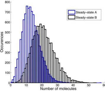
a1,a2,b1, andb2from the burst size data, nor measure them by other means. However, experience suggests that by supplementing the burst size distribution with other experimental data it may be possible to overcome the nonidentifiability of these parameters. This is reinforced by the observation that parameter combinations that lead to the sameAˆ2and hence the same burst size distribution can yield quite different steady-state distributions, as shown for example in Figure 4. The two steady state distributions shown Figure 2. Diagram of the generalised situation in which
intermediate, reversible stages are introduced. Here, G repre-sents an active gene, G* an active gene with a bound RNA polymerase, M an mRNA molecule, M* an mRNA molecule bound to a ribosome, P a protein, and S0 states which correspond to transcription factor unbinding and mRNA transcript decay.
have different choices of a1, a2, b1, and b2that yield the same value forAˆ2, and hence the same burst size distribution. However, the two steady state distributions are clearly different. This shows that steady state distribution data should allow us to distinguish between different combinations of parameters with the same Aˆ2, and hence potentially identify some or all of these parameters.
Empirical likelihood estimation. The main difficulty with such an approach is the lack of analytic expressions for the steady state distribution, making it impossible to derive an explicit formula for the likelihood. Instead one has to compute an estimate of the equilibrium distribution using simulations of the reaction
network [20] and then use these to derive an empirical likelihood by comparing to the experimental data. This can then be maximized in the usual way.
We applied this approach to the data from [7], which presents both burst size and steady state distributions for the same experimental system. In order to fully specify the steady state distribution, we need two additional parameters: the rate of transcription factor bindinga0and the rate of protein decay
b3. These do not enter into the expressions for the burst size distribution, and were assumed to be known (and fixed) for the simulations shown in Figure 4. In the absence of independent estimates of these parameters for theb-gal system, we explored the possibility of estimating these from the data in [7] directly by computing an empirical likelihood using simulation of the model (see below). We attempted both to maximize this empirical likelihood directly, and to obtain its distribution using Markov Chain Monte Carlo sampling. Neither of these approaches were successful with the full six parameter model (results not shown).
We can however, make use of independent estimates of parameters in the model to reduce the dimensionality of the parameter space. In effect this constrains the orginal optimization to a lower dimensional sub-space. We applied this approach with two different choices of parameter: the mRNA degradation rateb2 and the protein degradation rateb3.
Constraining on the mRNA degradation rate. We chose first to make use of the wide availability of estimates of the value of
b2, the rate of mRNA degradation. Since we also have the burst size data, we first estimateAˆ2and then use Equation 6 to obtain an expression fora2in terms ofa1,b1, andb2. We are left with the four dimensional parameter spacea0,a1,b1, andb3. At each point in this space, we simulate the model using the Gillespie algorithm to given an empirical estimate of the probabilityPn(a0,a1,b1,b3) of observingnproteins at equilibrium. This gives the empirical log-likelihood
Lða0,a1,b1,b3jDÞ~ X
n
DnlogðPnða0,a1,b1,b3ÞÞ:
whereDnis the number of times thatnproteins are observed in
the experimentally dataD.
Figure 3. Comparison of the distribution of experimentally measured burst sizes for the proteinsTsr-Venus(A)[6]and for theb-gal
(B)[7]with the standard model of gene expression.In both cases the blue line shows the best fit of the model to the data, obtained using the method of maximum likelihood givingAˆ2= 3.57 forTsr-VenusandAˆ2= 20.96 forb-gal. The error bars show the upper and lower bounds of the 95% confidence interval for the fitted parameter.
doi:10.1371/journal.pcbi.1000192.g003
Figure 4. Simulations of steady-state protein expression levels. For A we havea1= 0.018 andb1= 0.086 and for B we havea1= 0.009 andb1= 0.043, resulting in the sameAˆ2and hence identical burst size distributions. Other parameters werea0= 0.012,a2= 0.013,b2= 0.0039, and b3= 0.0007, based on previous simulation studies [22]. The distributions shown are for a run of 10,000 seconds using the Stocks implementation of Gillespie’s method [23], after an initial transient of 10,000 seconds. Previous studies have indicated that the steady state is in fact attained in under 1000 seconds.
Table 1.Means and standard deviations of estimates of the other parameters when the mRNA degradation rateb2set to 7.261023.
a0 a1 a2 b1 b3
m 0.0049 0.0017 0.1538 0.1210 (t1/2= 5.7 s) 0.0297 (t1/2= 23.3 s)
s 0.0052 0.0003 0.0088 0.0098 0.0098
These statistics are based on those runs that approached the global maximum (73.4% of all runs). These were selected by imposing a threshold atL=21350 and only considering those runs converging to a larger (more positive) likelihood. All reaction rates have units of s21.
doi:10.1371/journal.pcbi.1000192.t001
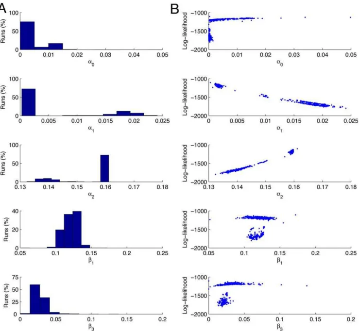
Figure 5. Parameter estimation results with fixed mRNA degradation rate.The results of 1000 runs of the Nelder-Mead maximisation of the log-likelihood for the parametersa0,a1,b1, andb3, witha2determined by the relationship in Equation 6, and with the mRNA degradation rateb2set to 7.261023, corresponding to a half-life forb-gal mRNA of 1.6 mins [24]. The panels in column A show the estimates of the values of the parameters and the percentage of times the Nelder-Mead algorithm converged to those values. The panels in column B are scattergrams of the values of the parameter estimates against the value of the log-likelihood. Each simulation is run 10,000 times to simulate a population of 10,000 cells, and each simulation is run for 5000 reaction steps. The starting values for the optimisation routine are: a0= 0.01 s21, a1= 0.02 s21, b1= 0.1 s21, and
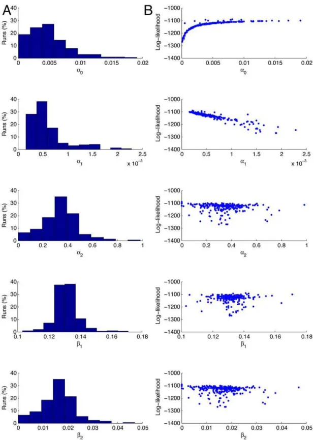
Figure 6. Parameter estimation results with fixed protein degradation rate.The results of 10,000 runs of the Nelder-Mead maximisation of the log-likelihood for the parametersa0,a1,b1, andb2, witha2determined by the relationship in Equation 6, and with the protein degradation rate set,b3set to 2.7761024, consistent with a half-life forb-gal 60 mins. The panels in column A show the estimates of the values of the parameters and the percentage of times the Nelder-Mead algorithm converged to those values. The panels in column B are scattergrams of the values of the parameter estimates against the value of the log-likelihood. Each simulation is run 10,000 times to simulate a population of 10,000 cells, and each simulation is run for 5000 reaction steps. The starting values for the optimisation routine are: a0= 0.01 s21, a1= 0.02 s21, b1= 0.1 s21, and
This empirical likelihood function can be maximized using any suitable optimization algorithm. Because it is computed using stochastic simulations any particular realization of the function is not smooth, making algoritms that use gradient (or Hessian) information unsuitable. We therefore opted to use the Nelder-Mead (simplex) method [21] with the results shown in Figure 5.
We can see that the likelihood has a local maximum at L<21800, and the simplex method frequently gets stuck in this region. However the majority of runs (73.4%) converge to the presumed global maximum. The means and standard deviations of the estimated parameter values are shown in Table 1. The value obtained forb3is 0.0297 s21, which corresponds to a half-life of 23 seconds. This appears to be unrealistically short, since b -galactosidase is a stable protein with a reported lifetime of hours. One possible explanation of this discrepancy is that the reported mRNA degradation rate b2= 7.261023 is always measured in experimental conditions where the gene is active. On the other hand, the burst size and equilibrium distributions in [7] are obtained under conditions where the gene is suppressed. It is possible that the mRNA degradation rates are significantly different in the two cases. To explore this hypothesis, we approached the problem from an alternative direction, fixing the protein degradation rate b3 to correspond to a half-life of 1 hour, and estimating the remaining five parameters, including mRNA degradation rateb2.
Constraining on the protein degradation rate. We therefore fixed b3to 1.926102
4 s21
, corresponding to a protein half-life of one hour, and then used same method as described above to estimate the other parametersa0,a1,a2,b1, andb2. We ran 10,000 simulations, as a relatively low number of runs converged (23.37%), with the others becoming trapped in a region with physically unrealistic (negative) reaction rates, and a log-likelihood ofL<22100. Of the runs which converged, 2057 (88%) converged to a local maximum at L<29150, while 279 (12%) converged to the presumed global maximum atL<21100. The results for the runs which converged can be seen in Figure 6, whilst summary statistics for the runs which converged to the presumed global maximum are presented in Table 2.
Comparison of the estimates. The transcription factor binding rate a0 is almost unchanged under both assumptions. When we fix the protein degradation rate in the second set of estimates to a value much lower than estimated in the first set we find that the transcription rate (i.e., rate of RNA polymerase binding) a1, is approximately one third of the previous value, decreasing from 0.0017 s21
to 0.0006 s21
, whilst the translation rate,a2shows an approximate two-fold increase, from 0.1538 s21 to 0.3352 s21
. It is intuitively reasonable that such a combination of decreasing transcription and increasing translation leads to the same overall level of protein expression. The parameterb1, the rate at which the transcription factor unbinds increases slightly, leading to shorter bursts. The increase in the mRNA degradation rate,b2from the original assumption of 0.007 s21to the estimate of 0.0161 s21
(corresponding to an mRNA half life of approximately 43 seconds) suggests that when expression of the gene is being strongly repressed as in this situation, there may well
be active degradation of the mRNA. It would be interesting to experimentally investigate this biologically significant prediction.
Discussion
We have shown that it is possible to use results from queuing theory to derive the burst size distribution of protein molecules produced by a single transcription factor binding event in terms of physically measurable kinetic rate constants for both the simplest model of gene expression, the so-called Standard Model, and for a number of natural extensions.
Furthermore, we have shown that the mathematical form of these models is nonidentifiable, and all such burst size distributions are actually determined by a single parameter. This implies that it is impossible to use burst size data alone to determine the relative contributions of transcription and translation to the variability in gene expression.
One possible way of overcoming this limitation is to use a combination of burst size data and steady-state data. However, this requires estimates of a further two parameters (which are not needed when using burst-size data alone). We were unable to estimate all six parameters directly from the combined data. However, using independent estimates of either the mRNA lifetime or the protein lifetime reduces the number of parameters by one, and enables successfully estimation of the remaining five parameters by maximizing an empirical likelihood using the Nelder-Mead simplex algorithm. Although this suffers from the common problem of occasional convergence to a local maximum, by using computing repeated estimates it was possible to identify and exclude such cases and hence obtain good estimates of the desired five kinetic parameters under the different constraints.
Supporting Information
Text S1 Derivation of probabilities.
Found at: doi:10.1371/journal.pcbi.1000192.s001 (0.10 MB PDF)
Author Contributions
Conceived and designed the experiments: PJI MPHS JS. Wrote the paper: PJI JS. Performed the analysis: PJI.
References
1. Elowitz MB, Levine AJ, Siggia ED, Swain PS (2002) Stochastic gene expression in a single cell. Science 297: 1183–1186.
2. Raser JM, O’Shea EK (2005) Noise in gene expression: origins, consequences, and control. Science 309: 2010–2013.
3. McAdams H, Arkin A (1997) Stochastic mechanisms in gene expression. Proc Natl Acad Sci U S A 94: 814–819.
4. Thattai M, van Oudenaarden A (2001) Intrinsic noise in gene regulatory networks. Proc Natl Acad Sci U S A 98: 8614–8619.
5. Raser JM, O’Shea EK (2004) Control of stochasticity in eukaryotic gene expression. Science 304: 1811–1814.
6. Yu J, Xiao J, Ren X, Lao K, Xie XS (2006) Probing gene expression in live cells, one protein molecule at a time. Science 311: 1600–1603.
7. Cai L, Friedman N, Xie XS (2006) Stochastic protein expression in individual cells at the single molecule level. Nature 440: 358–362.
8. Rigney D, Schieve W (1977) Stochastic model of linear, continuous protein synthesis in bacterial populations. J Theor Biol 69: 761–766.
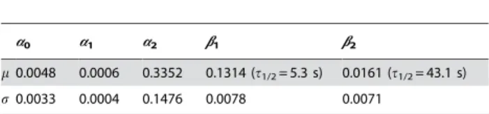
Table 2.Means and standard deviations of the parameter estimates, when the protein degradation rateb3set to 1.9261024(t1/2= 3600 s).
a0 a1 a2 b1 b2
m0.0048 0.0006 0.3352 0.1314 (t1/2= 5.3 s) 0.0161 (t1/2= 43.1 s)
s0.0033 0.0004 0.1476 0.0078 0.0071
These statistics are based on those runs which approached the global maximum (12% of converging runs). These were selected by imposing a threshold atL=22500 and only considering those runs converging to a larger (more positive) likelihood. All reaction rates have units of s21.
9. Berg OG (1978) A model for the statistical fluctuations of protein numbers in a microbial population. J Theor Biol 71: 587–603.
10. Paulsson J (2004) Summing up the noise in gene networks. Nature 427: 415–418. 11. Paulsson J (2005) Models of stochastic gene expression. Phys Life Rev 2:
157–175.
12. Paulsson J (2000) Stochastic Focusing: fluctuation enhanced sensitivity of intracellular regulation. Proc Natl Acad Sci U S A 97: 7148–7153.
13. Ho¨fer T, Malte RJ (2005) On the kinetic design of transcription. Genome Inform 16: 73–82.
14. Friedman N, Cai L, Xie XS (2006) Linking stochastic dynamics to population distribution: an analytical framework of gene expression. Phys Rev Lett 97: 168302.
15. Ho¨fer T, Nathansen H, Lohning M, Radbruch A, Heinrich R (2002) GATA-3 transcriptional imprinting in Th2 lymphocytes: a mathematical model. Proc Natl Acad Sci U S A 99: 9364–9368.
16. Hayot F, Jayaprakash C (2005) A feedforward loop motif in transcriptional regulation: induction and repression. J Theor Biol 234: 133–143.
17. Bailey NTJ (1964) The Elements of Stochastic Processes. New York: Wiley. 18. Timmer J, Muller TG, Swameye I, Sandra O, Klingmuller U (2004) Modelling
the nonlinear dynamics of cellular signal transduction. Int J Bifurcat Chaos 14: 2069–2079.
19. Sontag ED (2002) For differential equations with r parameters, 2r+1 experiments are enough for identification. J Nonlinear Sci 12: 553–583.
20. Gillespie DT (1977) Exact stochastic simulation of coupled chemical reactions. J Phys Chem 81: 2340–2361.
21. Ingram PJ, Stumpf MPH, Stark J (2006) Network motifs: structure does not determine function. BMC Genomics 7: 108.
22. Kierzek AM, Zaim J, Zielenkiewicz P (2001) The effect of transcription and translation initiation frequencies on the stochastic fluctuations in prokaryotic gene expression. J Biol Chem 276: 8165–8172.
23. Khachatourians GG, Tipper DJ (1974) Inhibition of messenger ribonucleic acid synthesis in Escherichia coli by thiolutin. J Bacteriol 119: 795–804.