The 2009–2010 arctic stratospheric winter

(1)

ACPD

11, 32535–32582, 2011

The 2009–2010 arctic stratospheric winter

A. D ¨ornbrack et al.

Title Page

Abstract Introduction

Conclusions References

Tables Figures

◭ ◮

Back Close

Full Screen / Esc

Printer-friendly Version Interactive Discussion

Discussion

P

a

per

|

Dis

cussion

P

a

per

|

Discussion

P

a

per

|

Discussio

n

P

a

per

|

Atmos. Chem. Phys. Discuss., 11, 32535–32582, 2011 www.atmos-chem-phys-discuss.net/11/32535/2011/ doi:10.5194/acpd-11-32535-2011

Atmospheric Chemistry and Physics Discussions

This discussion paper is/has been under review for the journal Atmospheric Chemistry and Physics (ACP). Please refer to the corresponding final paper in ACP if available.

– general evolution, mountain waves and

predictability of an operational weather

forecast model

A. D ¨ornbrack1, M. C. Pitts2, L. R. Poole3, Y. J. Orsolini4, K. Nishii5, and H. Nakamura5

1

Institut f ¨ur Physik der Atmosph ¨are, DLR Oberpfaff_{enhofen, 82230 Oberpfa}ff_enhofen,

Germany

2

NASA Langley Research Center, Hampton, Virginia 23681 USA

3

Science Systems and Applications, Incorporated, Hampton, Virginia 23666 USA

4

Norwegian Institute for Air Research, Kjeller, Norway

5

Research Center for Advanced Science and Technology, University of Tokyo, Tokyo, Japan

Received: 24 October 2011 – Accepted: 15 November 2011 – Published: 9 December 2011

Correspondence to: A. D ¨ornbrack (andreas.doernbrack@dlr.de)

(2)

ACPD

11, 32535–32582, 2011

Title Page

Tables Figures

◭ ◮

Back Close

Full Screen / Esc

Discussion

P

a

per

|

Dis

cussion

P

a

per

|

Discussion

P

a

per

|

Discussio

n

P

a

per

|

Abstract

The relatively warm 2009–2010 Arctic winter was an exceptional one as the North Atlantic Oscillation index attained persistent extreme negative values. Here, selected aspects of the Arctic stratosphere during this winter inspired by the analysis of the international field experiment RECONCILE are presented. First of all, and as a kind

5

of reference, the evolution of the polar vortex in its diff_{erent phases is documented.} Special emphasis is put on explaining the formation of the exceptionally cold vortex in mid winter after a sequence of stratospheric disturbances which were caused by upward propagating planetary waves. A major sudden stratospheric warming (SSW) occurring near the end of January 2010 concluded the anomalous cold vortex period.

10

Wave ice polar stratospheric clouds were frequently observed by spaceborne remote-sensing instruments over the Arctic during the cold period in January 2010. Here, one such case observed over Greenland is analysed in more detail and an attempt is made to correlate flow information of an operational numerical weather prediction model to the magnitude of the mountain-wave induced temperature fluctuations. Finally, it is

15

shown that the forecasts of the ECMWF ensemble prediction system for the onset of the major SSW were very skilful and the ensemble spread was very small. However, the ensemble spread increased dramatically after the major SSW, displaying the strong non-linearity and internal variability involved in the SSW event.

1 Introduction

20

The purpose of this study is to present a brief overview of the evolution of the Arctic stratospheric polar vortex during the 2009–2010 winter, to discuss the quality of the stratospheric forecasts of the European Centre of Medium Range Weather Forecasts (ECMWF) numerical weather prediction model IFS1, and to analyse mountain-wave

1

(3)

ACPD

11, 32535–32582, 2011

Title Page

Tables Figures

◭ ◮

Back Close

Full Screen / Esc

Discussion

P

a

per

|

Dis

cussion

P

a

per

|

Discussion

P

a

per

|

Discussio

n

P

a

per

|

induced stratospheric temperature anomalies over Greenland. During the 2009–2010 Arctic winter, airborne observations in the stratosphere were conducted during the in-ternational RECONCILE2campaign. This four-year research project was implemented by the European Union for comprehensive and detailed investigations of key processes governing Arctic ozone depletion. As a main research tool, the Russian high-altitude

5

research aircraft M55 GEOPHYSIKA3 (Stefanutti et al., 1999) was deployed in two distinct phases, with eight flights from 17–28 January 2010 and four flights in the sec-ond phase from 27 February–5 March 2010. For both phases, the aircraft was based in Kiruna, Sweden. The GEOPHYSIKA was equipped with sophisticated in-situ and remote-sensing instruments to probe the chemical composition and particle

distribu-10

tions and properties in the polar stratosphere. Additionally, during this winter space-borne CALIPSO (Cloud-Aerosol Lidar and Infrared Pathfinder Satellite Observations) measurements of polar stratospheric clouds (PSCs) revealed remarkable properties in cloud extent and structure; see e.g. Pitts et al. (2011), Koshrawi et al. (2011) and other papers in this special issue.

15

The northern polar vortex exhibits remarkable interannual variability. During the 2009–2010 winter, the sequence of a cold mid-winter vortex followed by a major sud-den stratospheric warming (SSW) near the end of January 2010 led to a variety of interesting phenomena during the two field phases of RECONCILE. From a dynami-cal viewpoint, probably the most interesting question of this stratospheric winter is why

20

such a strong and persistent polar vortex evolved from mid December 2009 until the

transformation dynamical core with a linear Gaussian transform grid and a triangular truncation. A finite element discretization is employed in the vertical direction, see also Hortal (2002) and Untch and Hortal (2004).

2

“Reconciliation of essential process parameters for an enhanced predictability of Arctic stratospheric ozone loss and its climate interactions” – a multinational project funded under the European Commission 7th Framework Programme; see https://www.fp7-reconcile.eu .

3

(4)

ACPD

11, 32535–32582, 2011

Title Page

Tables Figures

◭ ◮

Back Close

Full Screen / Esc

Discussion

P

a

per

|

Dis

cussion

P

a

per

|

Discussion

P

a

per

|

Discussio

n

P

a

per

|

end of January 2010 although many disturbances occurred earlier in November and December 2009 (e.g. Wang and Chen, 2010; Cohen et al., 2010). This question will be answered by investigating the evolution of the Western Pacific teleconnection patterns as described by Orsolini et al. (2009) and Nishii et al. (2010). We will investigate the subsequent major SSW, classify its development according to the zonal-mean

diag-5

nostics developed by Charlton and Polvani (2007) as a displacement or splitting type of warming, and, finally, answer the question: was the 2009–2010 Arctic stratospheric winter really unusually cold?

A refined classification of the CALIPSO observations by Pitts et al. (2011) enabled the identification of wave ice PSCs. Especially, during January 2010, wave ice PSCs

10

were frequently observed over and downstream of orographic obstacles in Greenland, northern Scandinavia, and Novaya Zemlya. Pitts et al. (2011) juxtaposed CALIPSO wave ice observations with a flow diagnostic derived from operational ECWMF anal-yses, namely horizontal divergence DIV, frequently used as a dynamical indicator of internal gravity waves, see for example Plougonvon et al. (2003). For a selected time

15

period in January 2010, reasonable correspondence was found by Pitts et al. (2011) be-tween wave ice PSC detections and local divergence/convergence whose magnitude exceeds a certain threshold. Here, we explore one case of CALIPSO mountain-wave induced PSC observations in more detail and investigate the quantitative relationship between DIV magnitude and stratospheric temperature anomalies. Furthermore,

for-20

ward and backward trajectories are calculated to demonstrate the long-distance impact local wave sources can have on the temperature history of air parcels.

For the first time, and in addition to the familiar usage of deterministic forecasts, the operational forecasts of the ECMWF ensemble prediction system (EPS) are analysed to provide quantitative measures of the reliability of the stratospheric forecasts. As

25

(5)

ACPD

11, 32535–32582, 2011

Title Page

Tables Figures

◭ ◮

Back Close

Full Screen / Esc

Discussion

P

a

per

|

Dis

cussion

P

a

per

|

Discussion

P

a

per

|

Discussio

n

P

a

per

|

The paper is divided into five parts. After this Introduction, the methodology and the data sources are explained. Section 3 deals with thermodynamic aspects of the vortex evolution and the quality of the ECWMF forecasts. Section 4 presents the investigation of a particular mountain wave period at the beginning of the very cold vortex period, and the final section 5 presents conclusions.

5

2 Methodology

2.1 Meteorological analyses and forecasts

In this study, diff_{erent datasets are used. The ‘truth’ is represented by either} opera-tional analysis or by ERA-Interim reanalysis data (Dee et al., 2011)4. Moreover, short-and medium-range forecasts from two diff_{erent sources are used: operational}

high-10

resolution deterministic forecasts and the lower-resolution control forecasts from the ECMWF ensemble prediction system. In addition to the control run, the EPS consists of 50 diff_{erently initialised members. During the 2009–2010 winter (on 26 January} 2010, to be precise), ECMWF upgraded the horizontal resolutions of its determin-istic forecast and data assimilation systems and of the EPS. The resolution of the

15

deterministic model was increased from T_L799L91 (∼25 km grid, p_TOP=₀_._{01 hPa) to}

T_L1279L91 (∼16 km, p_TOP=₀_._{01 hPa); the EPS resolution changed from} _T

L399L62

(∼56 km,p_TOP=_{5 hPa) to}_T

L639 L62 (∼32 km,pTOP=5 hPa) for the first 10 days of the

forecasts. For further details on how the operational forecasting system evolved before this update, see, for example, Tables I and II in Jung and Leutbecher (2007) or

con-20

sult the ECMWF web site (http://www.ecmwf.int). In addition to the ECMWF data, the analysis of the Western Pacific (WP) index was performed using the reanalysis data of

4

(6)

ACPD

11, 32535–32582, 2011

Title Page

Tables Figures

◭ ◮

Back Close

Full Screen / Esc

Discussion

P

a

per

|

Dis

cussion

P

a

per

|

Discussion

P

a

per

|

Discussio

n

P

a

per

|

the Japan Meteorological Agency (JMA) and the Central Research Institute of Electric Power Industry (CRIEPI), JRA25 reanalysis, see Onogi et al. (2007).

2.2 Measures for gravity wave activity

Locations of stratospheric gravity wave activity are derived from the ECMWF horizontal wind divergence (DIV) at 30 hPa. As discussed in Plougonven et al. (2003), the

iden-5

tified waves may not have the correct wavelengths and frequencies (due to the limited spatial and horizontal resolution), but the time and location of the waves as well as their phase orientation are expected to be relevant for studying their generation and propa-gation processes. In contrast to earlier studies using DIV to provide some qualitative indications of the horizontal structure of the waves, we attempt to relate the magnitude

10

of the horizontal wind divergence to the temperature fluctuations relevant for the gen-eration of PSCs, see Sect. 3.3. As an additional diagnostic tool for determining the temperature fluctuations due to the adiabatic cooling and warming in mountain-wave induced temperature anomalies, we analyze ensembles of trajectories calculated with the Lagrangian trajectory model LAGRANTO (Wernli and Davies, 1997).

15

2.3 CALIPSO data

For the case study provided in Sect. 3.3, spaceborne lidar measurements from CALIPSO provide the diff_{erent PSC compositions observed along the selected orbits.} The primary instrument on CALIPSO is a lidar (CALIOP, or Cloud-Aerosol Lidar with Orthogonal Polarization) that measures backscatter at wavelengths of 1064 nm and

20

532 nm, with the 532-nm signal separated into orthogonal polarization components parallel and perpendicular to the polarization plane of the outgoing laser beam. A de-scription of CALIOP and its on-orbit performance can be found in Hunt et al. (2009), and details on calibration of the CALIOP data are provided by Powell et al. (2009). CALIOP has proven to be an excellent system for observing PSCs (Pitts et al., 2007,

25

(7)

ACPD

11, 32535–32582, 2011

Title Page

Tables Figures

◭ ◮

Back Close

Full Screen / Esc

Discussion

P

a

per

|

Dis

cussion

P

a

per

|

Discussion

P

a

per

|

Discussio

n

P

a

per

|

The CALIPSO PSC algorithm as defined by Pitts et al. (2009) defined four CALIPSO PSC composition classes: supercooled ternary solution (STS), water ice, and two classes (Mix 1 and Mix 2) of liquid/nitric acid trihydrate (NAT) mixtures. Mix 1 de-notes mixtures with very low NAT number densities (from about 3×10−4cm−3 to 10−3cm−3), while Mix 2 denotes mixtures with higher (>10−3cm−3) NAT number

den-5

sities. Prompted by CALIOP observations during the recent winters, Pitts et al. (2011) defined two new PSC classes. Besides one additional NAT PSC class as referred to as Mix 2 enhanced, Pitts et al. (2011) found that intense mountain-wave induced PSCs can be distinguished as a subset of CALIPSO ice PSCs through their distinct optical signature inR₅₃₂_,the ratio of total to molecular backscatter at 532 nm, and the

10

lidar colour ratio, the ratio of 1064-nm particulate backscatter to 532-nm particulate backscatter. In general, lidar colour ratio is an indicator of the particle size; cirrus and tropospheric clouds have colour ratios of around 1, indicating large particles, while smaller aerosol particles have lower colour ratios (Liu et al., 2004). Over most of the ice PSC domain, the maximum number of observations occurs at colour ratios from 0.75

15

to 1.0, indicating large particles. But for ice PSCs with 1/R₅₃₂<0.02, the maximum in the number of observations shifts abruptly to colour ratios of 0.25 to 0.435 (see Fig. 2 in Pitts et al., 2011). As shown by Pitts et al. (2011), this behaviour is consistent with mountain-wave induced PSCs having high ice particle number densities (∼100 % ice activation from the background aerosol) but relatively small particles (1–1.5 µm radius).

20

Therefore, and because of their correspondence with the location of a dynamical indi-cator of mountain waves, the CALIPSO ice cloud observations with 1/R₅₃₂<0.02 are interpreted as mountain wave PSCs. Note that the CALIPSO wave ice PSC class is not all-inclusive; other CALIPSO ice PSC observations may be associated with mountain waves, but do not meet the strict (1/R₅₃₂<0.02) wave ice identification criterion, e.g.

25

(8)

ACPD

11, 32535–32582, 2011

Title Page

Tables Figures

◭ ◮

Back Close

Full Screen / Esc

Discussion

P

a

per

|

Dis

cussion

P

a

per

|

Discussion

P

a

per

|

Discussio

n

P

a

per

|

3 Results

3.1 Polar vortex evolution

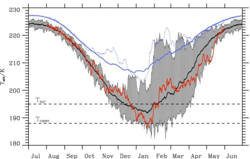
The temporal evolution of the minimum temperatureTMIN at the 50 hPa pressure

sur-face between 65◦N and 90◦N during the 2009–2010 Arctic winter is compared to the recent 21-year climatology in Fig. 1. Cooling of the Arctic polar vortex generally

fol-5

lowed the 21-year ECMWF climatological mean through mid November 2009, when

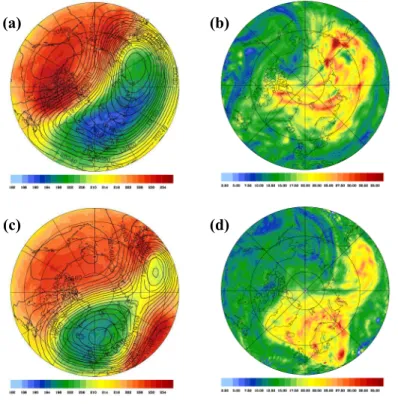
T_MIN had dropped to about 200 K (Fig. 1). From mid November until mid December 2009,T_MIN was well above the climatological mean. This period was characterized by downward propagating temperature anomalies in the stratosphere (see Fig. 4 in Wang and Chen, 2010 and Sect. 3.2). As a consequence of these disturbances, the polar

10

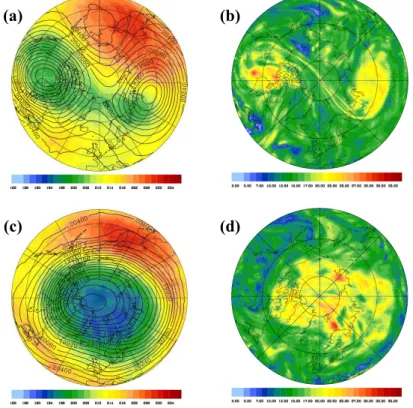
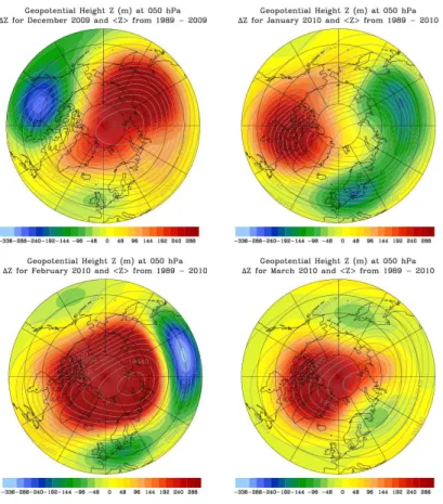
vortex split into two unequally strong lobes during the first ten days of December. Fig-ure 2 (a, b) illustrates the corresponding flow and temperatFig-ure structFig-ure of the polar vortex. The associated minor warming prevented a further decline of T_MIN, resulting in the observedT_MIN values above the climatological mean. The stronger and colder vortex lobe located over the Canadian sector of the Arctic survived this early warming

15

event, recovered and cooled gradually through mid-January 2010. There was a signif-icant drop inT_MINbelow T_NAT andT_FROST during this period, to values as much as 9 K below the climatological mean (Fig. 1). Typical flow and temperature fields from this exceptionally cold period are shown in Fig. 2 (c, d), depicting a coherent polar vortex centred near the North Pole. An analysis for the physical mechanisms leading to this

20

period is presented in Sect. 3.2.

During the second half of January 2010, a planetary wave-number-one event dis-placed the polar vortex towards the European sector of the Arctic (see Fig. 3a, b). This major warming event marked the start of the gradual break-up of the polar vortex. Al-though the vortex rapidly lost its symmetry and the cold region progressively shifted

25

(9)

distur-ACPD

11, 32535–32582, 2011

Title Page

Tables Figures

◭ ◮

Back Close

Full Screen / Esc

Discussion

P

a

per

|

Dis

cussion

P

a

per

|

Discussion

P

a

per

|

Discussio

n

P

a

per

|

bance of the polar vortex through the planetary wave activity resulted in a continuous warming in February 2010. Fig. 3 (c, d) depicts the stratospheric flow and temperature fields in early February 2010, several days before the final vortex break-up.

The mean polar cap temperature T_{POLAR CAP} in 2009–2010 (blue lines in Fig. 1) evolved in a qualitatively similar evolution as did T_MIN. However, and in contrast to

5

T_MIN, T_{POLAR CAP} indicated the onset of the warming earlier as a result of the vortex displacement from the pole. Furthermore, the mean polar cap temperature remained above the climatological mean for a longer period, until the end of March 2010. This means, that the Arctic stratosphere as a whole was warmer than usual, but that there were small regions within the vortex withT_MIN below the climatological mean in March

10

2010.

Another interesting feature during this period was the frequent occurrence of wave-like structures, discernable as undulations of the geopotential height fields in the ex-treme cold region over Greenland’s east cost (Fig. 2c, d). The associated regional cooling resulted from the adiabatic expansion in updrafts induced by orographic gravity

15

waves excited by the flow across Greenland. A case study will be discussed in detail in Sect. 4. According to the WMO definition5, a sudden stratospheric warming occurs

5

It must be noted that the so called WMO definition of sudden stratospheric warmings has been interpreted diff_{erently in details by di}ff_{erent authors. Andrews et al. (1987) writes: “It}

is defined somewhat arbitrarily, to be amajor warming if at 10 mb or below the zonal-mean temperature increases poleward from 60◦ latitude and the zonal-mean zonal wind reverses. If the temperature gradient reverses there but the circulation does not, it is defined to be a minor warming.”. Kr ¨uger et al. (2005) specify the North pole as the exact location where the temperature gradient∆_T=_T

90◦_N–T₆₀◦_Nhas to be calculated: “Major warmings are associated with a breakdown of the polar vortex as well as a warming of the polar region and the reversal of the meridional temperature gradient between 60◦latitude and the Pole. The vortex breakdown is defined by the reversal of the mean zonal westerlies poleward of 60◦latitude into easterlies, at least down to 10 hPa.” On the other hand, Limpasuvan et al. (2004) modified the criteria three ways by taking 85◦N and adding a 5 days period for which ∆_T=_T

(10)

ACPD

11, 32535–32582, 2011

Title Page

Tables Figures

◭ ◮

Back Close

Full Screen / Esc

Discussion

P

a

per

|

Dis

cussion

P

a

per

|

Discussion

P

a

per

|

Discussio

n

P

a

per

|

when the zonal mean zonal wind at 60◦N on the 10 hPa pressure surface becomes easterly. The first day on which the daily zonal-mean zonal wind at 60◦N and 10 hPa is easterly is defined as the central date of the warming (Charlton and Polvani, 2007, hereafter CP07). During the Arctic winter 2009–2010, the central date was determined to be 26 January 2010 (see Fig. 4b). Additionally, the WMO definition requires that the

5

10 hPa zonal-mean temperature gradient between 60◦N and 85◦N be positive for an event to be designated as major warming (see Limpasuvan et al., 2004, p. 2588). This condition was already satisfied exactly 5 days before the central date (see Fig. 4a). CP07 used 90◦N as the northernmost reference latitude to calculate the meridional zonal-mean temperature gradient; conducting the same analysis with temperatures

10

taken at this latitude does not change our results. No days within 20 days of the central date can be defined as SSW (vertical dashed lines at 15 February 2010 in Fig. 4). According to the WMO definition, the final warming occurred during the second half of February when the zonal-mean zonal wind became easterly and did not return to westerly for 10 days from 16 February until 26 February 2010. This is in agreement

15

withTMINandTPOLAR CAPat 50 hPa being well above the climatological mean.

In addition to the operational ECMWF analyses, Fig. 4 also displays the temporal evolution of the operational deterministic and the EPS control forecasts for a lead time of 120 h for both of the SSW criteria. Although the operational forecasts predict the onset of the major SSW event accurately, there exist some discrepancies between the

20

forecasts and the verifying analyses, especially after the major SSW end of January, which will be discussed in Sect. 3.3.

Based on a composite analysis, CP07 classified SSWs into vortex displacement and splitting events. Figure 5 depicts the 2009–2010 polar cap temperature anomaly

(11)

ACPD

11, 32535–32582, 2011

Title Page

Tables Figures

◭ ◮

Back Close

Full Screen / Esc

Discussion

P

a

per

|

Dis

cussion

P

a

per

|

Discussion

P

a

per

|

Discussio

n

P

a

per

|

∆_T

POLAR CAP for different pressure levels in a manner analogous to Fig. 6 in CP07.

Here,∆_T

POLAR CAP is calculated as the deviation to the temporal mean of the zonally

averagedT_{POLAR CAP}between 50◦N and 90◦N for the winter months DJFM. The evolu-tion of∆_T

POLAR CAPat 10 hPa (black solid line in Fig. 5) corresponds qualitatively to the

characteristic curve, CP07 calculated for the vortex displacement type as a composite

5

average. During the growth phase of the anomaly, the minimum∆_T

POLAR CAP occurs

about 25 days before the maximum ∆_T

POLAR CAP. The ∆TPOLAR CAP decrease in the

decay phase is within 3 K of the values found for the vortex displacement composite of CP07. However, the strength of the anomaly with∆_T

POLAR CAP≈17 K is about twice the

values calculated by CP07. This certainly reflects the fact that the composite

diagnos-10

tic of CP07 is an average over 15 events. Also astonishing is the temporal shift of the positive anomaly after the central date of the major SSW unlike in the CP07 analysis where it occurred exactly at the central date. In contrast to CP07, we do not observe an extended decay phase at lower levels (see dashed line in Fig. 5). Instead, the polar cap anomalies are amplified in the second half of February 2010. This is consistent

15

with the splitting of the polar vortex in this time period; see the supplementary material. In summary, we conclude that the SSW end of January 2010 resembles the displace-ment type. The eventual vortex break up into two lobes occurred in the second half of February 2010.

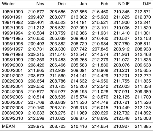
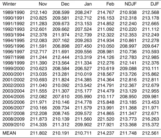
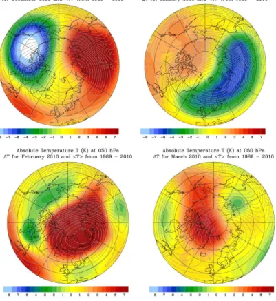
A climatological analysis to explore the question of whether this winter was

excep-20

tionally cold revealed the surprising result that the 2009–2010 winter was the second (third) warmest winter in the last 21 years at 30 hPa (50 hPa), see Tables 1 and 2, re-spectively. Only the period from the end of December 2009 until the end of January 2010 was colder than the climatological mean. This result is also confirmed by the negative stratospheric temperature anomalies in the diff_{erent winter months as shown}

25

(12)

ACPD

11, 32535–32582, 2011

Title Page

Tables Figures

◭ ◮

Back Close

Full Screen / Esc

Discussion

P

a

per

|

Dis

cussion

P

a

per

|

Discussion

P

a

per

|

Discussio

n

P

a

per

|

3.2 Strong vortex event of early January

The first phase of the RECONCILE flight campaign took place from the middle to end of January 2010. In the lower stratosphere, the coldest conditions in the entire win-ter occurred then, in a brief period between the two strong stratospheric warming events of December and late January. We now examine in some details the origin

5

and development of this pronounced cold vortex event. The vortex averaged temper-ature T_{POLAR CAP} at 50 hPa was anomalously cold from late December to early Jan-uary, and local temperatures fell below T_NAT, and even below T_FROST for a few days (Fig. 1). This period was the only occurrence of minimum vortex temperatures below

T_NAT during the entire winter (Fig. 1). On two occasions between December and

Febru-10

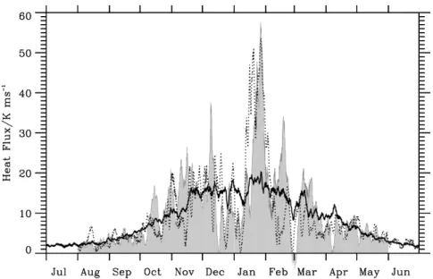
ary, the zonal-mean zonal winds at 10 hPa and 60◦N strengthened markedly to over 40 m s−1(Fig. 4b). The polar stratospheric cooling and vortex strengthening were likely a response of the weakened planetary wave activity which is indicated by the zonally-averaged meridional eddy heat flux decreasing well below its climatological average. Indeed, a period of anomalous low heat flux prevailed from mid-December to early

15

January (Fig. 8).

These two events when the polar stratosphere cooled and the vortex strengthened correspond to the development of a positive phase of the Western Pacific (WP) tele-connection pattern in the troposphere, as described by Orsolini et al. (2009) and Nishii et al. (2010). Generally, the Western Pacific pattern is characterized by a north-south

20

oriented dipole of geopotential anomalies in the troposphere, with a high over the North Pacific in its positive phase. The WP typical development and influence on the strato-spheric circulation is revealed by the composites of 18 strong events in the JRA re-analyses over the years 1979 to 2008, as described in Nishii et al. (2010). It involves the westward retrogression of the high over the North Pacific, where it interacts and

ul-25

(13)

ACPD

11, 32535–32582, 2011

Title Page

Tables Figures

◭ ◮

Back Close

Full Screen / Esc

Discussion

P

a

per

|

Dis

cussion

P

a

per

|

Discussion

P

a

per

|

Discussio

n

P

a

per

|

and 30 hPa within 5 days of the peak of the WP event, and the cooling persisted for a month.

Calculation of a standardized WP index using an Empirical Orthogonal Function ap-proach applied to the JRA re-analyses reveals that the period from December 2009 to early January 2010 was characterized by a positive WP index, with a first maximum

5

occurring around 13 December and a second, stronger maximum around 3 January (Fig. 9). In agreement with the ECMWF data, the heat flux anomalies with respect to the 1980–2007 JRA climatology over mid and high latitudes were negative during this period, and the coldest 50-hPa polar temperatures were found within a week of the peak in the WP index; see Figs. 8 and 9. Anomalously cold temperatures lasted

10

slightly less than 3 weeks, before the return to anomalously warm temperatures; see Fig. 1.

Five-day averaged geopotential heights for 1–5 January and 6–10 January are shown in Fig. 10, at 250 hPa and 30 hPa, separately, along with their anomalies from the 1980–2007 JRA climatology. In early January, a north-south dipole anomaly exists

15

at 250 hPa over the North Pacific/Eastern Eurasia region that project strongly onto the WP pattern in its positive phase (Fig. 10a). Additionally, a prominent positive tropo-spheric height anomaly (blocking high) is located over southern Greenland leading to tropospheric as well as stratospheric westerly winds. As they are nearly perpendicu-lar to Greenland’s east coast, the Atlantic block generated favourable flow conditions

20

for the excitation and propagation of mountain waves; see Sect. 4. At stratospheric altitudes, the reinforcing polar vortex is still slightly elongated and shifted off_{the pole} (Fig. 10b and compare to Fig. 2a).

From 6–10 January, following the peak in the WP index, the polar stratosphere at 30 hPa is characterised by lower heights than normal and a strong zonal circulation

25

(14)

ACPD

11, 32535–32582, 2011

Title Page

Tables Figures

◭ ◮

Back Close

Full Screen / Esc

Discussion

P

a

per

|

Dis

cussion

P

a

per

|

Discussion

P

a

per

|

Discussio

n

P

a

per

|

high over the North Atlantic (Fig. 10c). The upward propagation of the planetary waves into the stratosphere tends to be weakened by blocking highs over the Far East and western North Pacific but enhanced by blocking highs over the Euro-Atlantic sector. In other words, the Arctic stratosphere would have been developed even further if the Atlantic blocking had not formed simultaneously with the WP pattern; see Nishii et

5

al. (2011).

The interaction of the Pacific blocking high with the planetary wave trough appears clearly in the evolution of the potential vorticity (PV) depicted at the 300 K isentropic surface from late December 2009 to early January 2010 in Fig. 11, where the PV=₂ contour has been chosen to distinguish stratospheric (PV>2) from tropospheric air

10

(PV<2). Over the Far East, the westward-propagating block leads to a strong inward and poleward planetary wave breaking extruding an elongated high-PV filament into mid-latitudes. A similar pattern was found in the composite diagnostics by Nishii et al. (2010). Planetary wave breaking is the essence of the developing blocking high over the western Pacific and Fig. 11 illustrates how the breaking weakened the trough

15

over the Far East that is usually observed in winter seasons (Orsolini et al., 2009; Nishii et al., 2010).

Following this strong stratospheric cooling event, the transition to the major SSW came abruptly, without a preconditioning and weakening of the polar vortex (Fig. 4b; see also Ayarzag ¨uena et al., 2011). This particular SSW event was marked as an

20

extreme positive anomaly of wave-activity injection into the stratosphere in referring to Figs. 8 and 9.

3.3 Forecast quality

Based on the operational analyses in association with the ERA-Interim climatology from 1989–2009, the research aircraft GEOPHYSIKA was deployed in anomalously

25

(15)

ACPD

11, 32535–32582, 2011

Title Page

Tables Figures

◭ ◮

Back Close

Full Screen / Esc

Discussion

P

a

per

|

Dis

cussion

P

a

per

|

Discussion

P

a

per

|

Discussio

n

P

a

per

|

of the GEOPHYSIKA. The flight planning for an aircraft operating in the stratosphere proceeds in successive steps starting about 5 to 6 days before take-off_{. Therefore, the} medium-range forecasts of the ECMWF constituted a valuable tool for flight planning. During the daily weather briefings, the reliability of the operational deterministic fore-casts was often discussed. Subjectively, the impression arose that the variability of the

5

6–10 day forecasts for the stratosphere was exceptionally high and that the ECMWF IFS predicted the SSW too early for longer lead times.

In order to quantify the variability of the IFS forecasts, we analysed the performance of the 50 members of the EPS for two diff_{erent lead times during the winter 2009–2010.} First, we consider the variability of the EPS forecasts before evaluating the forecast’s

10

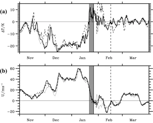
skill. Figures 12 and 13 show time series of the SSW criteria ∆_{T and U as well as} the ensemble spreads, calculated as the standard deviationsσ∆_T andσ_U (dotted lines

in panels a and b) at 10 hPa for forecast lead times of 240 h and 120 h, respectively. Additionally, the false alarm and hit rates6 of the EPS are shown for the period from November2009 till February 2010 (Figs. 12c and 13c).

15

For both lead times, the ensemble spreadsσ∆_T andσ_U are nearly uniform until the

onset of the SSW. Typical values in this pre-SSW period are σ∆T≈ 3 K (0.8 K) and σU≈5 m s−1 (1 m s−1) for the 240 h (120 h) forecasts, respectively. As expected, the

EPS spread decreases significantly for the shorter lead time in accordance with re-sults by Jung and Leutbecher (2007), compare Figs. 12 and 13. During the SSW,σ∆T 20

and σU decrease or remain nearly the same whereas after the SSW the ensemble

spreads increased by up to 500 %. This means, the forecasts containing the SSW period produce a larger uncertainty of flow regimes after the simulated SSW events occurred in the model simulations. Furthermore, the EPS forecasts also show a sig-nificant variability in the period of about 20 days after the central date of the SSW.

25

6

The false alarm rate is the ratio of false positive predictions to the sum of false positive and true negative predictions of the SSW criteria∆_{T >}_{0 and}_{U <}_{0, respectively. The hit rate is the}

(16)

ACPD

11, 32535–32582, 2011

Title Page

Tables Figures

◭ ◮

Back Close

Full Screen / Esc

Discussion

P

a

per

|

Dis

cussion

P

a

per

|

Discussion

P

a

per

|

Discussio

n

P

a

per

|

Summarizing, the forecast spread is relatively smaller for forecasts that start before the vortex weakening. In contrast, it is larger for forecasts that start when the observed vortex is weakening (late January). This means, the forecast system can capture well when the vortex begins to weaken, but it is diffi_{cult for the system to forecast how long} the vortex weakening will last by using rapidly changing fields as initial values for the

5

forecasts.

Surprising conclusions can be drawn from the analysis of the evolution of the hit and false alarm rates; see Figs. 12c and 13c. First of all, two distinct periods characterized either by high false alarm rates or high hit rates can be distinguished: the first period lasts from mid November until mid December 2009, and the second period covers the

10

SSW. For a lead time of 240 h, the false alarm rates for predicting a SSW in the first period are high, often equal to 1, i.e. all members of the EPS predict a positive ∆_T between the polar cap and mid latitudes. For the U-criterion, the false alarm rates are smaller, i.e. a significant portion of the EPS members does not predict flow reversal. Recall that this period was characterized by higher than normal planetary wave activity

15

(see Fig. 8), which might be responsible for the uncertainty in the EPS forecasts. For shorter lead times, the EPS forecasts have higher skill and the false alarm rates are limited to shorter periods in November (Fig. 13c).

Turning the attention to the SSW period, all EPS members (hit rate=_{1) predict the} onset and evolution of the SSW for the criteria∆_{T >}_{0 very accurately, whereas about}

20

half of the members satisfy the criteria U <0. This surprisingly uniform performance of the EPS holds for both lead times. In this period, the ensemble mean follows very closely the verifying analyses and the false alarm rate is low. Prior to the SSW, the false alarm rate is small for both criteria and restricted to a short period before the central date of the SSW. In contrast, the period after the SSW is characterized by large

25

(17)

ACPD

11, 32535–32582, 2011

Title Page

Tables Figures

◭ ◮

Back Close

Full Screen / Esc

Discussion

P

a

per

|

Dis

cussion

P

a

per

|

Discussion

P

a

per

|

Discussio

n

P

a

per

|

to be associated with the oscillations seen in the meridional heat flux. This leads to the question as to how realistic the forecasts are. Generally, the EPS members underes-timate the strength of the polar vortex as theU-values of the operational analyses are almost always larger than the ensemble mean (the only exception is the SSW period). This may be a result of the reduced horizontal resolution of the EPS, as a comparison

5

with Fig. 4b shows a satisfactory agreement between the U-values of the more highly resolved deterministic forecasts and the analyses.

In order to quantify the deviations between the 120 h and 240 h (EPS as well as de-terministic) forecasts and the verifying analyses, we calculated the meridional temper-ature diff_erence ∆_T

50 as zonally averaged temperature differences between the polar 10

cap (75◦N–90◦N) and the mid-latitudes (50◦N–65◦N) at 50 hPa for NDJF, see Fig. 14. Except for minor deviations, the∆_T

50 curves show the characteristic properties of the

∆_T _{curves depicted in Figs. 12a and 13a for the respective lead time. As already} indi-cated, the largest deviations (|∆_T

50|max≈10 K) between the forecasts and the verifying

analyses occur in two periods from mid-November until mid-December 2009 and after

15

the SSW in February 2010. This finding holds for both of the lead times considered (see Fig. 14c) and is in accordance with the high false alarm rates for the criterion∆_T_> 0 during these periods. As above, enhanced planetary wave activity and incorrect flow responses of the model simulations to the stratospheric warming are possible causes. The high-resolution deterministic forecasts seem only to deviate from the EPS control

20

run in periods of enhanced planetary wave activity. From mid-December 2009 until the end of January 2010, both forecasts are close together.

Finally, we turn to the predictability of the strong vortex events, which followed the high WP positive phases. At a lead time of 120 h, the intensification of the negative meridional temperature gradient and of the jet strength are well predicted in the EPS

25

(18)

ACPD

11, 32535–32582, 2011

Title Page

Tables Figures

◭ ◮

Back Close

Full Screen / Esc

Discussion

P

a

per

|

Dis

cussion

P

a

per

|

Discussion

P

a

per

|

Discussio

n

P

a

per

|

4 Mountain wave-induced temperature anomalies

As already indicated in Sect. 3.2, west winds dominated the tropospheric as well as stratospheric flow at the beginning of January 2010. As shown in D ¨ornbrack and Leut-becher (2001), nearly unidirectional winds in the troposphere and stratosphere are one essential criterion for mountain waves propagating upward into the stratosphere.

5

Indeed, besides synoptic-scale ice PSCs inside the cold polar vortex, CALIPSO fre-quently observed wave ice PSCs with distinct properties in backscatter ratio, aerosol depolarisation, and colour ratio during the exceptionally cold period in January 2010.

Pitts et al. (2011) found a reasonable agreement of the locations of these wave ice PSCs and extreme values of DIV for a limited period from 31 December 2009–

10

14 January 2010. In a hydrostatic model such as the IFS, localized anomalies of the divergence above a certain threshold, e.g.|DIV|=₂_×₁₀−4_s−1 _{at 30 hPa, are} suit-able dynamical indicators of updrafts and downdrafts. Most of the events identified in early January 2010 could be directly linked to vertically propagating mountain waves as their geographical locations are in close proximity to steep orographic obstacles.

15

Figure 15 (left panel) shows mountain wave events also occurring during the months October/November/December 2009. However, compared to the signature found in Jan-uary 2010 (Fig. 15, right panel) their locations are more widespread and the frequency is smaller. Furthermore, there are no CALIPSO reports of wave ice PSCs during the months in 2009. If we accept the given threshold of the horizontal divergence as

indica-20

tor of mountain waves, Greenland, northern Scandinavia, Iceland, and Novaya Zemlya can be identified as the most active locations for stratospheric mountain waves during the 2009–2010 winter.

Figure 16 shows CALIPSO observations of mountain-wave induced PSCs over the east coast of Greenland on 4 January 2010 for two diff_{erent orbit tracks, one parallel}

25

(Fig. 16a) and the other nearly perpendicular (Fig. 16b) to the coast line (see supple-mentary material of Pitts et al., 2011 for plots of the orbit tracks7). The general wind

7

(19)

ACPD

11, 32535–32582, 2011

Title Page

Tables Figures

◭ ◮

Back Close

Full Screen / Esc

Discussion

P

a

per

|

Dis

cussion

P

a

per

|

Discussion

P

a

per

|

Discussio

n

P

a

per

|

direction is west, i.e. Fig. 16a shows PSC observations almost perpendicular and Fig 16b observations nearly parallel to the prevailing westerly winds8. Superimposed are Θ_and_T _{interpolated in space and time along the orbit tracks from the ECMWF} opera-tional analyses. Both the wavy structure inΘ_{and the tilted stratospheric temperature} minimum as well as the vertically tilted coherent ice region reveal patterns of mountain

5

wave-induced PSCs as observed over Scandinavia by airborne lidar (D ¨ornbrack et al., 2002). The PSC composition changed along the orbit track and along the main wind direction (wind is blowing from right to left in Fig. 16b): upstream the PSC was domi-nated by liquid STS clouds whereas NAT mixtures occur downstream of the ice PSCs. A similar composition change was also observed by airborne lidar measurements; see

10

for example Fig. 10 in D ¨ornbrack et al. (2002). Figure 16a illustrates this finding along the south-north oriented cross-section parallel to Greenland’s coastline. Depending on the distance of the track from the upstream mountains the composition changes from south to north: directly over the mountains ice clouds formed, further north and down-stream from Greenland’s mountains ice and NAT mixtures dominated whereas liquid

15

STS clouds existed at the northernmost part of the orbit which was not influenced by the mountains of Greenland.

In order to investigate the relationship between the divergence and the correspond-ing temperature fluctuations quantitatively, we consider the months of December 2009 and January 2010. A stratospheric box was defined to cover parts of Greenland from

20

60◦N. . . .85◦N and 60◦W. . . .20◦W and isentropic surfaces between 430 K and 610 K. ECMWF operational analyses were interpolated to the isentropic surfaces on lati-tude/longitude grids with two diff_{erent horizontal resolutions of 0.25}◦_{and 2.50}◦_, respec-tively. The time series of the minimum temperatureT_MIN and the minimum/maximum

8

(20)

ACPD

11, 32535–32582, 2011

Title Page

Tables Figures

◭ ◮

Back Close

Full Screen / Esc

Discussion

P

a

per

|

Dis

cussion

P

a

per

|

Discussion

P

a

per

|

Discussio

n

P

a

per

|

horizontal divergence DIV_MINand DIV_MAX and the standard deviations9σ_DIVandσ_T in this particular domain are plotted for selected isentropic levels in Fig. 17. Periods of en-hanced magnitude of DIV_MIN and DIV_MAX are associated with a temporal decrease in

T_MINand increased temperature standard deviationsσ_T. Generally, the negative DIV_MIN values have a larger magnitude than the positive DIV_MAX for both plotted resolutions.

5

However, the magnitude of DIV_MIN_/_MAX and T_MIN is larger for the higher resolution of 0.25◦. Especially in the period at the beginning of January 2010, enhanced values of|DIV_MIN_/_MAX|>2×10−4s−1 correspond to stratospheric temperature decreases as-sociated with mountain wave induced cooling (compare the period around 4 January 2010 and Fig. 16). Based on these results, the period 2 . . . 4 January 2010 has been

10

selected to study the relationship of DIV and T in more detail as another mountain wave event of similar strength was also observed by CALIPSO on 2 January 2010, see supplementary material in Pitts et al. (2011).

Figure 18a and b present correlations between the minimum temperatureT_MIN and the minimum and maximum horizontal divergences, DIV_MIN and DIV_MAX over

Green-15

land for equidistantly distributed isentropic levels between 430 K and 610 K in the period from 2-4 January 2010 on two regular latitude/longitude grids with 2.50◦and 0.25◦ reso-lution, respectively. As already indicated above,TMINreaches lower (more extreme)

val-ues at the higher resolved grid, especially, at the uppermost stratospheric levels. The magnitude of the correlation coeffi_{cients for the regression functions} _T

MIN=f(DIVMIN) 20

and TMIN=f(DIVMAX) increase from 0.34 and −0.27 for 2.50◦ to 0.46 and −0.42 for

0.25◦ resolution, respectively. Thus, there is a correlation between the minimum tem-perature and the magnitude of the divergence wherebyT_MIN remains stronger corre-lated with DIV_MIN. The correlation between TMIN and DIVMIN/MAX can be increased

in two ways: by restricting the analysis to upper stratospheric levels or by reducing

25

the sample domain to the region where the mountains waves actually occurred. For example, if one only considers stratospheric levels between 570 K and 610 K, the

mag-9

(21)

ACPD

11, 32535–32582, 2011

Title Page

Tables Figures

◭ ◮

Back Close

Full Screen / Esc

Discussion

P

a

per

|

Dis

cussion

P

a

per

|

Discussion

P

a

per

|

Discussio

n

P

a

per

|

nitudes of the correlation coeffi_{cients increase to 0.76 and} ₋_{0.74, respectively (not} shown) whereas the domain reduction to an area between 60◦N . . . 70◦N, 40◦W . . . 20◦W results in an increase to 0.53 and−0.62 (see Fig. 18c).

Finally, Fig. 18d shows the same data for the reduced sample domain as in Fig. 18c but plotted for regional anomalies of the minimum temperatureT_MIN and the extreme

5

values of DIV:∆_T =_T

MIN–TAVE =f(∆DIV−) and∆T=f(∆DIV +

) with ∆_DIV−=_DIV

MIN–

DIV_AVE and ∆_DIV+=_DIV

MAX – DIVAVE, where DIVAVE is the mean divergence in the

sample domain. Here, the correlation coeffi_{cients are 0.54 and} ₋_{0.82, respectively.} Therefore, extreme values of the magnitude of horizontal divergence |DIV_MIN_/_MAX| above a certain threshold (for example 2×10−4s−1) can serve as a suitable dynamical

10

indicator of gravity wave-induced temperature anomalies in the stratosphere. Espe-cially, Fig. 18d shows that the magnitude of the anomalies∆_T _{increases nearly linearly} with growing|∆_DIV+/−_|_{. The separation of points by isentropic levels found in panels} (a)–(c) is due to the temperature decrease for increasing altitude. It disappears when we plot the anomalies∆_T_{, and the random distribution of points demonstrates the}

ir-15

regular impact of gravity-wave induced cooling and warming in the height range under consideration (Fig. 18d).

Lagrangian forward and backward trajectories were calculated for the mountain wave event of 4 January 2010 over Greenland. Figure 19 shows the multiscale response of the altitude and temperature histories along the trajectories starting at 20 hPa (Fig. 19a)

20

and 40 hPa (Fig. 19b) in the reduced sample region which covers that of the observed PSCs depicted in Fig. 16. As 4 January 2010 is approached, the parcels’ temperatures decrease although there is no significant rise in altitude. This synoptic-scale cooling is due to the cold area of the polar vortex the parcels gradually approach. Additionally, mountain wave-induced cooling and warming and the associated displacements in the

25

(22)

ACPD

11, 32535–32582, 2011

Title Page

Tables Figures

◭ ◮

Back Close

Full Screen / Esc

Discussion

P

a

per

|

Dis

cussion

P

a

per

|

Discussion

P

a

per

|

Discussio

n

P

a

per

|

The minimum temperature attains extreme values, here, especially for the trajectories released at 20 hPa. Altogether, the structure of the temperature fluctuations changes from the time before the gravity wave event to the time after. In the mean, the maximum and minimum heating and cooling rates show larger magnitudes after the wave event. This means, disturbances due to the wave event propagate with the mean wind and

5

might impact the PSC formation/evolution downstream.

5 Conclusions

The EC funded project RECONCILE explored essential physical and chemical pro-cesses for improving the predictability of Arctic stratospheric ozone loss by means of an aircraft field experiment during the Arctic winter 2009–2010. The campaign forecasts

10

for the research flights into the stratosphere as well as the post-campaign analyses of the in-situ and remote-sensing observations inspired most of the topics investigated in this paper.

Here, we overview and document the evolution of the Arctic polar vortex employing high resolution operational ECMWF analyses. We found that the stratospheric winter

15

evolved in diff_{erent phases: planetary wave disturbances in November/early December} prohibited a quick early cooling and kept the minimum stratospheric temperatures well above the climatological mean. After a vortex split in early December, the formation of a strong and cold polar vortex dominated the evolution from mid-December 2009 to the end of January 2010. It was shown that the formation of this exceptionally cold

20

and strong mid-winter polar vortex could be traced back to the intensification of the WP teleconnection pattern. A major SSW marked the end of the cold period. After being markedly displaced from the pole, the vortex eventually split into two lobes, with one lobe surviving until mid-March 2010 when the second phase of RECONCILE campaign concluded. A climatological analysis revealed that the 2009–2010 winter was one of the

25

(23)

ACPD

11, 32535–32582, 2011

Title Page

Tables Figures

◭ ◮

Back Close

Full Screen / Esc

Discussion

P

a

per

|

Dis

cussion

P

a

per

|

Discussion

P

a

per

|

Discussio

n

P

a

per

|

For the first time, the ensemble prediction system has been analysed to investigate the forecast skill of the ECMWF IFS. It was shown that the 240 h forecasts provide a reliable means to predict the onset and the process of the SSW. The false alarm rate was low and almost all members of the ensemble predicted the correct evolution (high hit rate). However, after the warming happened, the ensemble predictions deviated

5

significantly leading to a high ensemble spread. In accordance with the findings of Jung and Leutbecher (2002), we also found a remarkable reduction of ensemble spread for a reduced lead time of 120 h.

During mid-winter, especially in January 2010, wave ice PSCs were frequently iden-tified in the CALIPSO measurements. Here, a typical CALIPSO observation of a

10

mountain-wave event over Greenland was analysed in more detail. The currently avail-able spatial resolution of about 16 km provided by the operational ECMWF numerical weather prediction model IFS10 allows estimates of the temperature anomalies, cool-ing rates and their persistence downstream of the mountains for resolved gravity waves with horizontal wavelengths larger than about 100 km. In particular, a correlation

be-15

tween stratospheric temperature anomalies and the magnitude of the horizontal diver-gence could be derived. It was shown that the magnitude of the diverdiver-gence is directly proportional to the temperature anomaly in a limited area surrounding the resolved mountain waves.

The authors are aware that the diff_{erent topics presented in this paper have not been}

20

completely explored and that all possible details have not been elaborated. Each of the topics investigated could be the subject of a research paper on its own. For example, to elucidate the contributions of the diff_{erent planetary wave numbers to the} strato-spheric warming event and its subsequent evolution more precisely could be one topic to be explored. More case studies relating the magnitude of the horizontal divergence

25

10

This horizontal resolution of an operational global model amounts approximately to the resolution which was used for studying regional mesoscale eff_{ects on the dynamics and}

(24)

ACPD

11, 32535–32582, 2011

Title Page

Tables Figures

◭ ◮

Back Close

Full Screen / Esc

Discussion

P

a

per

|

Dis

cussion

P

a

per

|

Discussion

P

a

per

|

Discussio

n

P

a

per

|

field to stratospheric temperature anomalies could lead to simple parameterizations of gravity-wave induced impacts on particle formation for use in global circulation mod-els. Nevertheless, we think that this paper might be a useful reference for all those who participated in the RECONCILE campaign and those who are interested in the diff_erent subjects of the paper.

5

Supplementary material related to this article is available online at: http://www.atmos-chem-phys-discuss.net/11/32535/2011/

acpd-11-32535-2011-supplement.zip.

Acknowledgements. The field activities in Kiruna, as well as the meteorological support and analysis, were funded by the EC as part of the FP7 project RECONCILE (Grant number:

10

RECONCILE-226365-FP7-ENV-2008-1. We thank Hal Maring, NASA Radiation Sciences Pro-gram manager, and Dr. David Considine, NASA ProPro-gram Scientist for the CALIPSO/CloudSat Missions for their continued support of CALIPSO PSC research (MP, LP). Support for L. Poole is provided under NASA contract NNL11AA00B. The ECMWF data were available through the special project “Eff_{ect of non-hydrostatic gravity waves on the stratosphere above Scandinavia”}

15

by one of the authors (A.D.).

References

Andrews, D. G., Holton, J. R., and Leovy, C. B.: Middle Atmosphere Dynamics, Academic Press, 489 pp., 1987.

Ayarzag ¨uena, B., Langematz, U., and Serrano, E.: Tropospheric forcing of the stratosphere:

20

A comparative study of the two diff_{erent major stratospheric warmings in 2009 and 2010, J.}

Geophys. Res., 116, D18114, doi:10.1029/2010JD015023, 2011.

Carslaw, K. S., Wirth, M., Tsias, A., Luo, B. P., D ¨ornbrack, A., Volkert, A., Leutbecher, M., Renger, W., Bacmeister, J. T., Reimer, E., and Peter, T.: Increased stratospheric ozone depletion due to mountain-induced atmospheric waves, Nature, 391, 675–678, 1998.

25

(25)

ACPD

11, 32535–32582, 2011

Title Page

Tables Figures

◭ ◮

Back Close

Full Screen / Esc

Discussion

P

a

per

|

Dis

cussion

P

a

per

|

Discussion

P

a

per

|

Discussio

n

P

a

per

|

Cohen, J., Foster, J., Barlow, M., Saito, K., and Jones, J.: Winter 2009–2010: A case study of an extreme Arctic Oscillation event, Geophys. Res. Lett., 37, L17707, doi:10.1029/2010GL044256, 2010.

Dee, D. P., Uppala, S. M., Simmons, A. J., Berrisford, P., Poli, P., Kobayashi, S., Andrae, U., Balmaseda, M. A., Balsamo, G., Bauer, P., Bechtold, P., Beljaars, A. C. M., van de Berg,

5

L., Bidlot, J., Bormann, N., Delsol, C., Dragani, R., Fuentes, M., Geer, A. J., Haimberger, L., Healy, S. B., Hersbach, H., H ólm, E. V., Isaksen, L., K ˚allberg, P., K öhler, M., Matricardi, M., McNally, A. P., Monge-Sanz, B. M., Morcrette, J.-J., Park, B.-K., Peubey, C., de Rosnay, P., Tavolato, C., Th épaut, J.-N., and Vitart, F.: The ERA-Interim reanalysis: configuration and performance of the data assimilation system, Q. J. R. Meteorol. Soc., 137, 553–597,

10

doi:10.1002/qj.828, 2011.

D ¨ornbrack, A. and M. Leutbecher: Relevance of mountain waves for the formation of polar stratospheric clouds over Scandinavia: A 20 year climatology, J. Geophys. Res., 106, 1583– 1593, 2001.

D ¨ornbrack, A., Leutbecher, M., Volkert, H., and Wirth, M.: Mesoscale forecasts of stratospheric

15

mountain waves, Meteorol. Appl., 5, 117–126, 1998.

D ¨ornbrack, A., Birner, T., Fix, A., Flentje, H., Meister, A., Schmid, H., Browell, E. V., and Mahoney, M. J.: Evidence for inertia gravity waves forming polar stratospheric clouds over Scandinavia, J. Geophys. Res., 107, 8287, doi:10.1029/2001JD000452, 2002.

Eckermann, S. D., D ¨ornbrack, A., Vosper, S. B., Flentje, H., Mahoney, M. J., Bui, T. P., and

20

Carslaw, K. S.: Mountain wave-induced polar stratospheric cloud forecasts for aircraft sci-ence flights during SOLVE/THESEO 2000, Weather Forecast., 21, 42–68, 2006.

Hanson, D. and Mauersberger, K.: Laboratory studies of the nitric acid trihydrate: Implications for the south polar stratosphere, Geophys. Res. Lett., 15, 855–858, 1988.

Hinssen, Y. B. L. and Ambaum, M. H. P.: Relation between the 100 hPa heat fux and

strato-25

spheric potential vorticity, J. Atmos. Sci., 67, 4017–4027, 2010.

Hortal, M.: The development and testing of a new two-time-level semi-Lagrangian scheme (SETTLS) in the ECMWF forecast model, Q. J. R. Meteorol. Soc., 128, 1671–1687, doi:10.1002/qj.200212858314, 2002.

Hunt, W. H, Winker, D. M., Vaughan, M. A., Powell, K. A., Lucker, P. L., and Weimer, C.:

30

CALIPSO Lidar Description and Performance Assessment, J. Atmos. Ocean. Technol., 26, 1214–1228, doi:10.1175/2009JTECHA1223.1, 2009.

(26)

ACPD

11, 32535–32582, 2011

Title Page

Tables Figures

◭ ◮

Back Close

Full Screen / Esc

Discussion

P

a

per

|

Dis

cussion

P

a

per

|

Discussion

P

a

per

|

Discussio

n

P

a

per

|

during winter, Q. J. R. Meteorol. Soc., 133, 1327–1340, 2007.

Khosrawi, F., Urban, J., Pitts, M. C., Voelger, P., Achtert, P., Kaphlanov, M., Murtagh, D., and Fricke, K.-H.: Denitrification and polar stratospheric cloud formation during the Arctic winter 2009/2010, Atmos. Chem. Phys. Discuss., 11, 11379–11415, doi:10.5194/acpd-11-11379-2011, 2011

5

Kr ¨uger, K., Naujokat, B., and Labitzke, K.: The Unusual Midwinter Warming in the Southern Hemisphere Stratosphere 2002: A Comparison to Northern Hemisphere Phenomena, J. Atmos. Sci., 62, 603–613, doi:10.1175/JAS-3316.1, 2005.

Lait, L. R.: An alternative form for potential vorticity, J. Atmos. Sci., 51, 1754–1759, 1994. Limpasuvan, V., Thompson, D. W. J., and Hartmann, D. L.: The Life Cycle of the Northern

10

Hemisphere Sudden Stratospheric Warmings, J. Climate, 17, 2584–2596, 2004.

Liu, Z., Vaughan, M. A., Winker, D. M.., Hostetler, C. A., Poole, L. R., Hlavka, D., Hart, W., and McGill, M.: Use of probability distribution functions for discriminating be-tween cloud and aerosol in lidar backscatter data, J. Geophys. Res., 109, D15202, doi:10.1029/2004JD004732, 2004.

15

Nishii, K., Nakamura, H., and Orsolini, Y. J.: Cooling of the wintertime Arctic stratosphere induced by the Western Pacific teleconnection pattern. Geophys. Res. Lett., 37, L13805, doi:10.1029/2010GL043551, 2010.

Nishii, K, Nakamura, H., and Orsolini, Y. J.: Geographical dependence observed in blocking high influence on the stratospheric variability through enhancement and suppression of

up-20

ward planetary-wave propagation, J. Climate, J. Climate, 24, 6408–6423, doi:10.1175/JCLI-D-10-05021.1, 2011.

Onogi K., Tsutsui, J., Koide, H., Sakamoto, M., Kobayashi, S., Hatsushika, H., Matsumoto, T., Yamazaki, N., Kamahori, H., Takahashi, K., Kadokura, S., Wada, K., Kato, K., Oyama, R., Ose, T., Mannoji, N., and Taira, R.: The JRA-25 reanalysis, J. Meteorol. Soc. Japan, 85,

25

369–432, 2007.

Orsolini, Y. J., Karpechko, A. Y., and Nikulin, G.: Variability of the Northern Hemisphere polar stratospheric cloud potential: The role of North Pacific disturbances, Q. J. R. Meteorol. Soc., 135, 1020–1029, doi:10.1002/qj.409, 2009.

Pitts, M. C., Thomason, L. W., Poole, L. R., and Winker, D. M.: Characterization of Polar

Strato-30

spheric Clouds with spaceborne lidar: CALIPSO and the 2006 Antarctic season, Atmos. Chem. Phys., 7, 5207–5228, doi:10.5194/acp-7-5207-2007, 2007.