Abstract—This paper presents an analysis on energy consumption and energy efficiency of a hexapod robot during its turning motion over flat terrain. The energy consumption model has been derived for statically stable wave-turning gaits by considering a minimization of dissipating energy for optimal foot force distribution. Two approaches, such as minimization of norm of feet forces and minimization of norm of joint torques have been developed. The variations of average power consumption and energy consumption per weight per traveled length with angular velocity and angular stroke have been studied for turning motion with tripod and tetrapod gait patterns. Tetrapod gaits are found to be more energy-efficient than the tripod gaits.
Index Terms—Dynamic model, Energy consumption, Hexapod robot, Turning motion
I. INTRODUCTION
NERGY consumption is one of the main restrictions for the use of walking robots in practical applications [1]. The minimization of energy consumption plays an important role in the locomotion of an autonomous multi-legged robot used for service applications. Several studies on walking energy consumption had been carried out in the field of robotics, biomechanics and zoology. Some of those are design of energy efficient mechanical leg structure [2], [3]; optimal selection of gait parameters [4], [5]; and optimal solution to foot force distribution [6], [7]. Orin and Oh [8] tried to resolve the foot force distribution for minimum energy consumption and load balance among several legs. Nahon and Angeles [9] used quadratic programming to minimize power of robotic systems actuated by DC motors, but considered power regeneration by the motors doing negative work. Marhefka and Orin [10] utilized quadratic programming to solve foot force distribution in hexapod walking robots that minimizes the power consumption in DC motors. In their work, gains from power regeneration by the DC motors were not permitted in the optimization problem. Kar et al. [11] performed an analysis of energy efficiency with respect to structural parameters, friction coefficient and duty factor of wave gaits, based on a simplified model of six-legged robot. Kar et al. [11] and Lin and Song [12] took the instantaneous power to be the product of instantaneous joint torques and joint velocities. Such modeling ignored the fact that a considerable amount
Manuscript received April 08, 2011.
Shibendu Shekhar Roy is with the Mechanical Engineering Department, National Institute Technology, Durgapur, WB, INDIA (corresponding author to provide phone: 91-343-2755278; fax: 91-343-2543447; e-mail:
of power is dissipated on the joints of the supporting legs. In order to eliminate such drawbacks, it is better to consider the integral of the sum of squares of the joint torques as a criterion of dissipated energy in the actuators. Nishii [13] used the integral of weighted sum of the product of instantaneous joint torques and joint velocities and the sum of squares of the joint torques as energetic cost, and analyzed the energetic cost of a two joint six-legged robot. Zhoga [14] and Zelinski [15] analyzed energy expenditure and energy efficiency of multi-legged locomotion systems taking into account the leg dynamics and torque, but they failed to consider joint actuator type, although the joint actuator’s contribution to energy consumption is decisive. The above mentioned work focused on walking along straight-forward path only.
During locomotion of a multi-legged robot on flat terrain, different types of gaits, namely straight forward gait, crab gaits and turning gaits etc. are to be used to avoid obstacles in its path. Out of many possible gait patterns, the present study concentrates on dynamic modeling and energy efficiency analysis of turning gaits, as turning motion is very important to omni-directional locomotion. Hirose et al. [16], Zhang and Song [17] analyzed turning motion of a multi-legged robot from kinematics point of view. The problem of optimal turning gait generation of a six-legged robot had been solved by Pratihar et al. [18] using a combined genetic algorithm and fuzzy logic approach. Pratihar et al. [19] extended this work to find optimal path and gait generation of a hexapod walking robot, but they considered a simplified model of the robot. Moreover, they did not consider a detailed dynamic behavior of the leg and trunk body, although its contribution to gait generation was significant. Due to the inherent complexity of a realistic walking robot, it is not an easy task to include inertial terms in the modeling. The most of the studies on walking robot dynamics were conducted with simplified models of legs and body. But, in order to have a better understanding of its walking, dynamics and other important issues of walking, such as dynamic stability, energy efficiency and its on-line control; kinematics and dynamic models based on a realistic walking robot design are necessary to build. To the best of the authors’ knowledge, no significant study has been reported on energy efficiency analysis of turning gaits of a realistic six-legged robot. In the present study, attempts are made to study the effects of turning gait parameters [16-17] on energy consumption of a real six-legged robot.
Dilip Kumar Pratihar is with the Mechanical Engineering Department, Indian Institute Technology, Kharagpur, WB, INDIA (e-mail:
Study on Energy Consumption in Turning
Motion of Hexapod Walking Robots
Shibendu Shekhar Roy, and Dilip Kumar Pratihar
II. MATHEMATICAL FORMULATION OF THE PROBLEM In order to develop a detailed dynamic and energy consumption model of a hexapod robot while negotiating turning motion on flat terrain, the following assumptions are made: (a) The trunk body is kept at a constant height from the level terrain and turning radius is also kept constant. (b) The robot is assumed to generate a wave-turning gaits with two duty factors equal to 1/2 (tripod gait) and 2/3 (tetrapod gait). (c) The joint actuators are DC geared motors, which cannot store negative energy. Therefore, any negative energy, i.e., gain in energy supplied by external forces, is lost.
A complete kinematic and dynamic model of a realistic hexapod robot is required to analyze the complex relationships between locomotion parameters and energy consumption.
A. Kinematic Model of the Hexapod Walking Robot
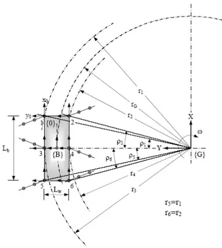
A 3-D model of a realistic hexapod walking robot, considered in the present study, is shown in Figure 1. Denavit-Hartenberg (D-H) notations [20] have been used in kinematic modeling of each leg of three degrees of freedom. Table I shows four D-H parameters, namely link length (ai), link twist (i), joint distance (di), and joint angle (i), which are required to completely describe three joint legs.
The foot tip reference frame {3} can be expressed in the leg reference frame {0} as follows:
3
0 0 1 2 i-1
3 1 2 3 i
i=1
T T T T T (1)
1 2 3 1 2 3 1 1 2 2 3 2 3 1
0 1 2 3 1 2 3 1 1 2 2 3 2 3 1 3
2 3 2 3 2 2 3 2 3
CθC(θ+θ) -CθS(θ+θ) Sθ L +L Cθ+L C(θ+θ) Cθ SθC(θ+θ) -SθS(θ+θ) -Cθ L +L Cθ+L C(θ+θ) Sθ T =
S(θ+θ) C(θ+θ) 0 L Sθ+L S(θ+θ)
0 0 0 1
The six legs and trunk body must be integrated to solve the kinematics problem of the robot. The body attached reference frame {B} is located at the geometric center of the trunk body as shown in Figure 2.
Body reference frame {B} and hip reference frame of ith leg {0i} are represented with respect to global reference frame {G} attached at turning center, using transformation matrix as given below.
G
G G
B
G C(-ωt) -S(-ωt) 0 r S(ωt) S(-ωt) C(-ωt) 0 r C(ωt) =
0 0 1 h
0 0 0 1
T
i i
i i G
0,i
G ib C(-ωt) -S(-ωt) 0 r S(ρ +ωt) S(-ωt) C(-ωt) 0 r C(ρ +ωt) =
0 0 1 h +h
0 0 0 1
T ; i=leg number
Here, ri is the path radius of hip of ith leg, which can be determined as follows:
2 2
w b
1 5 G
L L
r =r = r + +
2 2
;
2 2
w b
2 6 G
L L
r =r = r - +
2 2
;
w 3 G
L r = r +
2
;
w 4 G
L r = r
-2
;
-1 b 1 5
G w L ρ=ρ =tan
2r +L
,
-1 b 2 6
G w L ρ =ρ =tan
2r -L
; ρ3=ρ4=0, Fig. 1: 3-D model of a hexapod walking
fix
fiy
-fiz W
XB ZB
fix
fiy
-fiz
Leg 5
Leg 3
Leg 6
Leg 1
Leg 4
Leg 2 D-HPARAMETERS FOR TABLEI LEGS
Link no. ai i di i
1 L1=0.085m 90 0 1
2 L2=0.115m 0 0 2
3 L3=0.100m 0 0 3
‘+’ for left side legs, ‘-’ for right side legs
where rG is the turning radius of the CG of the trunk body, is the angular speed of the CG of the robot, t is the time, Lb is the length of the trunk body and Lw is the width of the trunk body.
The joint trajectory of the swing leg is assumed to follow a fifth-order polynomial in time (t). The jth joint of a swing leg, that is, j can be represented in fifth-order polynomial as follows:
j = aj0+aj1t+aj2t2+aj3t3+aj4t4+aj5t5 ; j=1, 2, 3. (2) where aj0, aj1, aj2, aj3, aj4, and aj5 are coefficients. The boundary conditions of joint angles, joint velocities and joint accelerations at initial and final points of the trajectory are applied to determine the six coefficients for each joint. The velocity and acceleration equations for each joint of a swing leg can be obtained using the following equations:
2 3 4
j j1 j2 j3 j4 j5
θ =a +2a t+3a t +4a t +5a t (3)
2 3
j j2 j3 j4 j5
θ=2a +6a t+12a t +20a t
(4)
Moreover, the velocity and acceleration equations of for each leg during the support phase can be expressed as follows: θ 1
= J p
and 1
( )
θ= J p Jθ
,
where Cartesian velocity vector T
x y [ -v -v 0 ]
p ,
joint velocity vector, T
1 2 3 [θ θ θ ]
θ and J is the Jacobian matrix.
B. Dynamic Model of the Hexapod Walking Robot
A six-legged robot is a complex linkage, where its legs are connected to one another through the trunk body and also through the ground, and thus, form closed kinematic chains. The equations of motion for such a complex mechanism with six legs, each of which has 3 degrees of freedom, are derived by applying Lagrangian dynamics formulation together with Denavit-Hartenberg’s link coordinate representation, and the derived relationships are given in the vector-matrix form as follows:
T
i i i i
τ = [M(θ)θ+ H(θ,θ) + G(θ)] - J F, (5)
where M() is the 33 mass matrix of the leg, H is a 31 vector of centrifugal and Coriolis terms, G() is a 31 vector of gravity terms, i is the 31 vector of joint torques
and Fi is the 31 vector of ground reaction forces of foot ‘i’.
During the leg’s swing phase, there is no foot-terrain interaction, and Fi becomes equal to zero. However, during
the support phase, ground contact exists and equation (5) becomes undetermined, which has to be solved using an optimization criterion, e.g., optimal foot force distribution. The dynamic equations of the mechanical part for each swing leg have been shown in Appendix.
For computing foot-force distributions, the following assumptions are made: (i) The ground legs are assumed to be supporting the trunk body without any slippage on their tip points. (ii) The contacts of the tips of the feet with ground can be modeled as hard point contacts with friction.
In the present study, the said problem of foot force distribution has been solved using two approaches as explained below.
Approach 1: Minimization of Norm of Feet Forces
To analyze the feet forces that robot must exert, let us assume that Fi=[fix, fiy, fiz]T is the ground-reaction force vector on foot i. The wrench W=[ Fx, Fy, Fz, Mx, My, Mz]T contains the forces (Fx, Fy, Fz) and moments (Mx, My, Mz) acting on the robot’s center of gravity and represents the robot’s payload, any externally applied forces and inertial effects of the robot’s body. However, the inertial effects of the legs have been neglected to simplify the study. Under these conditions, six equilibrium equations [21] that balance forces and moments can be expressed in matrix form as follows:
[A].[F] = - [B].[W] (6)
where 3 3 3
p q r 6 9 [ ]
I I I A =
R R R for tripod gait;
3 3 3 3
p q r s 6 12 [ ]
I I I I A =
R R R R for tetrapod gait;
and 3 3
c 3 6 6 [ ]
I 0
B =
R I
I3 is the (33) identity matrix, 03 is the (33) null matrix and Ri is the (33) skew symmetric matrix of vector [xi, yi, zi]T.
i i
i i i
i i
0 z y
z 0 x
y x 0
R and 3
1 0 0 0 1 0 0 0 1
I
This matrix defines the position of tip of a foot i (i=p, q, r for tripod gait or i=p, q, r, s for tetrapod gait) or that of center of gravity (i=c) with respect to body reference frame. The coordinates of ith foot-ground contact point with respect to body reference frame, located at the body’s geometric center, are denoted by (xi, yi, zi). The values of Fx, Fy, Fz, Mx, My and Mz for turning motion are to be found as: Fx= -FIx; Fy= mrG2; Fz=-mgz; and
B B 2
x xz yz
dω
M =- I + I ω
dt ;
B B 2
y yz xz
dω
M =- I - I ω
dt ;
B z zz
dω M = I
dt With the known feet positions, the feet forces during a whole locomotion cycle can be computed using equation (6), which is indeterminate, because it consists of six equations but there are more than six unknowns. The solution of equation (6) has been obtained using the least squared method, which gives the minimum norm solution of the indeterminate equilibrium equations.
Approach 2: Minimization of Norm of Joint Torques
In this approach, the equation (6) can be reformulated by using the following relations.
[F] = [D].[] (7)
where p
3 3 q
3 3
r
3 3 9 9
[ ]=
J 0 0
D 0 J 0
0 0 J
and p
3 3 3 q
3 3 3
r
3 3 3
s 3 3 3 12 12 [ ]=
J 0 0 0
0 J 0 0
D
0 0 J 0
0 0 0 J
for tetrapod gait;
-1
i T
i =
J J ; Ji is the (33) Jacobian matrix of leg i. Here, []=[p, q, r]T for tripod gait; []=[p, q, r, s]T for tetrapod gait, and i=[i1, i2, i3]T is the torque vector containing three joint torques at leg i.
The equation (6) can be rewritten as follows:
[A][D][] = - [B][W] (8)
[AJ][] = - [B][W] (9)
The minimum norm solution of the indeterminate equation (9) has been obtained using a least squared method.
C. Energy Consumption Model of the Hexapod Robot
The energy consumption in a legged robot is mainly due to the energy consumed by an actuator in each joint of the legs. As a joint is driven by a DC motor [20], the consumed energy in motor during a time (T) is given by:
T T T T 2
a a e a a
0 0 0 0
E=
u i dt
(u +R i ) i dt
dt
dt; (10) where ua is the applied voltage and ia is the armature current. The first term is mechanical energy and the second term is related to energy loss by heat emissions. Although a negative value for the first term, i.e., mechanical energy indicates a gain in energy supplied by external forces, DC motor cannot store this energy. Therefore, the energy consumed by the DC motor during time T is given by
T T 2
0 0
E=
dt
dt, (11) where
=0
Total energy consumed by all motors in a hexapod robot becomes
6 3T
2 ij ij ij 0
i 1 j 1
E= dt
(12)where 2 s 2 t RG =
K
; Gs is the speed ratio of the geared motor,
Kt is the torque constant, R is the armature resistance, ue is the induced voltage in the armature windings opposing the applied voltage.
III. SIMULATION RESULTS AND DISCUSSION
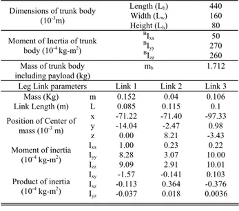
Results of computer simulations based on above formulations are discussed in detail. Table II shows the physical parameters of the hexapod walking robot considered in the present study. The values of moment of inertia and positions of centre of gravity of this real robot have been computed using CATIA CAD/CAE software. In this simulation, turning radius and body height are assumed to be equal to 1.0 m and 0.13 m, respectively.
Table III shows the average values of the squares of joint torques of the robot negotiating turning motion with tripod and tetrapod gaits, as obtained by approaches 1 and 2. Simulation results indicate that the average of the squares of joint torques during one complete locomotion cycle for tripod gait has turned out to be higher than that of tetrapod gait for both the approaches. The average value of the squares of joint torques of the robot as obtained by approach 1 is seen to be higher than that yielded by approach 2 for both tripod and tetrapod gaits. Since the average of the squares of joint torques is considered to be proportional to average dissipated power (average heat loss) of the joint motor, it can be concluded that approach 2 is more energy efficient than approach 1. This happens due to the forces required to support the body are distributed more evenly among the legs in case of tetrapod gait compared to tripod gait and thereby, the contribution (in terms of torque and power) of each support leg is reduced.
if 0 if 0
TABLEIII
AVERAGE VALUES OF THE SQUARES OF JOINT TORQUES DURING TURNING MOTION
Duty factor ()
Average of the squares of joint torques (N-m)2
Approach 1 Approach 2
1/2 7.2513 4.0773
2/3 5.5217 2.9939
Angular stroke=8°, Angular velocity = 2°/sec, Turning radius=1 m, TABLEII
PHYSICAL PARAMETERS OF THE HEXAPOD ROBOT
Dimensions of trunk body (10-3m)
Length (Lb)
Width (Lw)
Height (Lh)
440 160 80 Moment of Inertia of trunk
body (10-4 kg-m2)
BI xx BI
yy BI
zz
50 270 260 Mass of trunk body
including payload (kg)
mb 1.712
Leg Link parameters Link 1 Link 2 Link 3 Mass (Kg) m 0.152 0.04 0.106 Link Length (m) L 0.085 0.115 0.1 Position of Center of
mass (10-3 m)
x -71.22 -71.40 -97.33 y -14.04 -2.47 0.98 z 0.00 8.21 -3.43 Moment of inertia
(10-4 kg-m2)
Ixx 1.00 0.23 0.22
Iyy 8.28 3.07 10.00
Izz 9.09 2.91 10.01
Product of inertia (10-4 kg-m2)
Ixy -1.57 -0.141 0.103
Ixz -0.113 0.364 -0.376
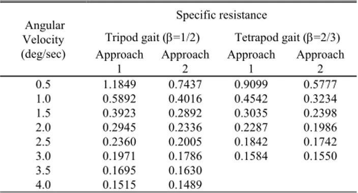
The effects of angular velocity on average power consumption over one locomotion cycle of the robot for two different duty factors are displayed in Table IV. For a particular value of duty factor, average power consumption is found to increase with the increase in angular velocity, as expected. Thus, the velocity should be as low as possible to minimize power consumption for a particular duty factor. However, traveling with a low velocity takes more time to cover a fixed distance, and consequently, total energy consumption may be increased. The energy required to travel a fixed distance can be quantified using a parameter called specific resistance [12], that is, energy consumed per unit weight and per unit traveled length. Table V displays the effects of variation of angular velocity on specific resistance during turning over a flat terrain. Specific resistance is found to decrease with the increase of angular velocity for a particular value of duty factor. However,
average power consumption is seen to increase with the increase in angular velocity. Moreover, for a high value of duty factor, angular velocity cannot be increased to a high value due to dynamic constraints of joint actuators. The blank cells of Tables IV and V correspond to angular velocities, angular strokes and duty factors at which the robot is unable to walk because of the violation of dynamic constraints of the motors. Approach 2 is seen to yield more efficient gaits compared to approach 1 for both the tripod and tetrapod gaits. Results related to the effects of angular stroke on average power consumption and specific resistance during turning of the robot with wave gaits of two different duty factors are presented in Tables VI and VII, respectively. For a given angular velocity, both average power consumption and specific resistance are found to increase with angular stroke for both tripod and tetrapod gaits. Moreover, for a particular angular stroke, average power consumption and specific resistance are seen to be higher for tripod gait than that of tetrapod gait for both approaches 1 and 2. It is interesting to observe that approach 2 has provided more energy efficient solutions compared to approach 1 for all angular strokes. Tetrapod gaits are found to be more energy-efficient compared to tripod gaits.
IV. CONCLUSIONS
An attempt has been made to minimize energy consumption of a hexapod robot during turning motion on flat terrain. An energy consumption model has been derived for statically stable wave-turning gaits by minimizing dissipating power for optimal foot force distribution and minimizing total energy expenditure for optimal selection of turning gait parameters, namely angular velocity, angular stroke and duty factor. It is important to mention that approach 2 (that is, minimization of norm of joint torques) is seen to be more energy efficient compared to approach 1 (that is, minimization of norm of feet forces) for both duty factors. The variations of average power consumption and specific resistance with angular velocity and angular stroke have been studied for turning motion of hexapod robot with two different duty factors. In order to minimize total energy consumption, the angular velocity should be as high as possible and angular stroke should be as low as possible, but without violating dynamic constraints of the joint motors. TABLEVI
VARIATIONS OF AVERAGE POWER CONSUMPTION WITH ANGULAR STROKE DURING TURNING MOTION
Angular Stroke (deg.)
Average power consumption (in Watts) Tripod gait (=1/2) Tetrapod gait (=2/3) Approach
1
Approach 2
Approach 1
Approach 2 8.0 0.3724 0.3107 0.2836 0.2569 7.0 0.3614 0.2951 0.2781 0.2472 6.0 0.3529 0.2800 0.2741 0.2380 5.0 0.3465 0.2656 0.2714 0.2294 4.0 0.3418 0.2519 0.2699 0.2215
3.0 0.3384 0.2391
Angular velocity=2 deg./sec, Turning radius=1 m
TABLEVII
VARIATIONS OF SPECIFIC RESISTANCE WITH ANGULAR STROKE DURING TURNING MOTION
Angular Stroke
(deg.)
Specific resistance
Tripod gait (=1/2) Tetrapod gait (=2/3) Approach
1
Approach 2
Approach 1
Approach 2 8.0 0.3107 0.2593 0.2366 0.2144 7.0 0.3016 0.2462 0.2321 0.2063 6.0 0.2945 0.2336 0.2287 0.1986 5.0 0.2891 0.2216 0.2264 0.1914 4.0 0.2852 0.2101 0.2252 0.1848
3.0 0.2824 0.1995
Angular velocity=2 deg./sec, Turning radius=1 m
TABLEIV
VARIATION OF AVERAGE POWER CONSUMPTION WITH ANGULAR VELOCITY DURING TURNING MOTION
Angular Velocity (deg/sec)
Average power consumption (in Watts) Tripod gait (=1/2) Tetrapod gait (=2/3) Approach
1
Approach 2
Approach 1
Approach 2 0.5 0.3520 0.2228 0.2722 0.1731 1.0 0.3521 0.2407 0.2726 0.1938 1.5 0.3527 0.2600 0.2728 0.2156 2.0 0.3529 0.2800 0.2741 0.2380 2.5 0.3535 0.3004 0.2760 0.2610 3.0 0.3544 0.3210 0.2848 0.2787
3.5 0.3555 0.3419
4.0 0.3631 0.3569
Angular stroke=6°, Turning radius=1 m TABLEV
VARIATION OF SPECIFIC RESISTANCE WITH ANGULAR VELOCITY DURING TURNING MOTION
Angular Velocity (deg/sec)
Specific resistance
Tripod gait (=1/2) Tetrapod gait (=2/3) Approach
1
Approach 2
Approach 1
Approach 2 0.5 1.1849 0.7437 0.9099 0.5777 1.0 0.5892 0.4016 0.4542 0.3234 1.5 0.3923 0.2892 0.3035 0.2398 2.0 0.2945 0.2336 0.2287 0.1986 2.5 0.2360 0.2005 0.1842 0.1742 3.0 0.1971 0.1786 0.1584 0.1550
3.5 0.1695 0.1630
4.0 0.1515 0.1489
APPENDIX Dynamics of Swing Leg
The swing leg of a legged robot can be studied from the dynamics point of view as a 3-DOF robotic manipulator with a foot as end-effector of the latter. Systematic derivation of the Lagrange-Euler equations yields the torque expressions as follows:
i i
τ = [M(θ)θ+ H(θ,θ) + G(θ)]
It can be written in a summation form as
n n n
i ik ikm k m i
k 1 k 1 m 1
M h G
θ
θ θ , i=1, 2, 3. where Mik is the inertia matrix, hikm is the Coriolis and centripetal forces matrix, Gi is the gravity loading vector and n is the number of joints. The terms: Mik, hikm and Gi can be obtained as follows:3
T
ik jk j ji
j max(i,k )
M Tr
U J U , i, k=1, 2, 3.3
T
ikm jkm j ji
j max(i,k ,m)
h Tr
U J U , i, k, m=1, 2, 3. 3j
i j ji j
j i
G m .
g U r, i=1, 2, 3.Here, g = [gx gy gz 0] is the acceleration due to gravity with respect to the reference coordinate system. Now, Uij and Uijk can be obtained as follows:
0 0 j 1i j 1 j i
ij
j
j
i
0
j
i
T
T Q
T
U
0 j 1 k 1
j 1 j k 1 k i
ij 0 k 1 j 1
ijk k 1 k j 1 j i
k
i k j
i j k
0 i j, i k
T Q T Q T
U
U T Q T Q T
where
j k
0 1 0 0
1 0 0 0
0 0 0 0
0 0 0 0
Q Q
ACKNOWLEDGMENT
The first author acknowledges all helps from Mr. Ajay Kr. Singh, Department of Mechanical Engineering, NIT, Durgapur, India.
REFERENCES
[1] S. M. Song, and K. J. Waldron, Machines That Walk: The Adaptive
Suspension Vehicle. The MIT Press, Cambridge, Massachusetts, USA,
1989.
[2] S.M. Song, V.J. Vohnout, K.J. Waldron, and G.L. Kinzel, “Computer-aided design of a leg for an energy efficient walking machine,”
Mechanism and Machine Theory, vol. 19, pp. 17-24, 1994.
[3] S. Hirose, and Y. Umetani, “Some consideration on a feasible walking mechanism as a terrain vehicle,” in Proc. of 3rd International
CISM-IFToMM Symposium, Udine, Italy, 1978, pp. 357-375.
[4] D. W. Marhefka, and D. E. Orin, “Gait planning for energy efficiency in walking machines,” in Proc. of IEEE international conference on
Robotics and Automation, Albuquerque, NM, April, 1997, pp. 474-
480.
[5] D.C. Kar, K.K. Issac, and K. Jayarajan, “Gaits and energetics in terrestrial legged locomotion,” Mechanisms and Machine Theory, vol. 38, no. 2, pp. 355–366, 2003.
[6] J.S. Chen, F.T. Cheng, K.T. Yang, F.C. Kung, and Y.Y. Sun, “Optimal force distribution in multilegged vehicles,” Robotica, vol. 17, pp. 159-172, 1999.
[7] C.A. Klein, and S. Kittivatcharapong, “Optimal force distribution for the legs of a walking machine with friction cone constraints,” IEEE
Transactions on Robotics and Automation, vol. 6, no. 1, pp. 73-85,
1990.
[8] D. E. Orin, and Y. Oh, “A mathematical approach to the problem of force distribution in locomotion and manipulation system containing closed kinematic chains,” in Proc. 3rd Int. CISM-IFToMM
Symposium, Udine, Italy, 1978, pp. 1-23.
[9] M. A. Nahon, and J. Angeles, “Minimization of power losses in cooperating manipulators,” ASME Journal of Dynamic, Systems,
Measurement and Control, vol. 114, pp. 213-219, 1992.
[10] D. W. Marhefka, and D. E. Orin, “Quadratic optimization of force distribution in walking machines,” in Proc. IEEE Int. Conf. Robotics
and Automation, Belgium, 1998, pp. 477–483.
[11] D. C. Kar, K. K. Issac and K. Jayarajan, “Minimum energy force distribution for a walking robot,” Journal of Robotic Systems, vol. 18, no. 2, pp. 47–54, 2001.
[12] B. S. Lin, and S. M. Song, “Dynamic modeling, stability and energy efficiency of a quadrupedal walking machine,” Journal of Robotic
Systems, vol. 18, no. 11, pp. 657–670, 2001.
[13] J. Nishii, “Gait pattern and energetic cost in hexapods,” in Proc. 20th
Annu. Int. Conf. IEEE Engineering in Medicine and Biology Society,
20, 1998, pp. 2430–2433.
[14] V. V. Zhoga, “Computation of walking robots movement energy expenditure,” in Proc. IEEE Int. Conf. Robotics and Automation, Belgium, 1998, pp. 163-168.
[15] T. Zelinska, “Efficiency analysis in the design of walking machine,”
J. Theor. Appl. Mech., vol. 38, pp. 693-708, 2000.
[16] S. Hirose, H. Kikuchi, and Y. Umetani, “The standard circular gait of a quadruped walking vehicle,” Advanced Robotics, vol. 1, no. 2, pp. 143- 164, 1986.
[17] C.D. Zhang, and S.M. Song, “Turning Gait of a Quadrupedal Walking Machine,” in Proc. of IEEE Int. Conf. on Robotics and Automation, Sacramento, California, April, 1991, pp. 2106-2112.
[18] D.K. Pratihar, K. Deb, and A. Ghosh, “Optimal turning gait of a six-legged robot using GA-fuzzy approach,” Artificial Intelligence for
Engineering Design, Analysis and Manufacturing, vol. 14, pp. 207–
219, 2000.
[19] D.K. Pratihar, K. Deb, and A. Ghosh, “Optimal path and gait generations simultaneously of a six-legged robot using a GA-fuzzy approach,” Robotics and Autonomous Systems, vol. 41, pp. 1-20, 2002.
[20] K.S. Fu, R.C. Gonzalez, and C.S.G. Lee, Robotics: Control, Sensing,
Vision, and Intelligence, Singapore: McGraw Hill, 1987.
[21] S.S. Roy, A.K. Singh, and D.K. Pratihar, “Analysis of six-legged walking robots,” in Proc. 14th National Conference on Machines and