M
ASTER IN
F
INANCE
Master Final Work
P
ROJECT
W
ORK
E
QUITY
R
ESEARCH
-
E
FACEC
F
ILIPA
D
IAS
F
IÚZA
O
LIVEIRA
M
ASTER IN
F
INANCE
Master Final Work
P
ROJECT
W
ORK
E
QUITY
R
ESEARCH
-
E
FACEC
F
ILIPA
D
IAS
F
IÚZA
O
LIVEIRA
S
UPERVISION OF
M
ASTER
’
S
T
HESIS
:
PROFESSOR Dr. CARLOS MANUEL COSTA BASTARDO
ABSTRACT
Efacec is a company that has undergone several changes, going from being a small industrial
company to the largest group in the electric field. Its core emphases are the international
market among its constant investment in innovation and new technologies. Furthermore, it
has a highly skilled workforce resulting in a persistent position at the forefront of the sectors
where it develops its activities.
The goal of this project is to determine the intrinsic value of Efacec’s shares, through a detailed
analysis of the operational performance of the company, its external environment and its
growth prospects. The valuation was based on the Free Cash Flow to Firm method, which
according to the literature review represents the best method to assess Efacec.
According to the assumptions defined, the firm value of Efacec is 401.666.793 euros and the
equity value is 12.457.793 euros (0,30 euros per share). Since Efacec is not a quoted company
the Price Earnings Ratio multiple was used to decide whether or not if investors should buy the
shares. Taking this into account, the indicator for Efacec of 1,51 is extremely low when
compared with its peer group (14,60). Consequently, Efacec’s share price is undervalued,
despite being considered one of the largest Portuguese multinationals. Thus the
recommendation is not to buy Efacec shares.
Keywords: Company Valuation, Discounted Cash Flow, Free Cash Flow to Firm, Enterprise
ACKNOWLEDGEMENTS
This project is the result of a long process of hard work, which would not been possible
without the support and dedication of all who accompanied me. In this way I want to express
my gratitude.
To Professor Carlos Bastardo, supervisor of this project, my sincere gratitude for his
monitoring and availability and for his wise guidance, support and critical opinion in the
elaboration of this project.
To my friends and colleagues, who always helped and motivated me in my academic career.
To Rodrigo Salema who gave me a precious hand in the revision of this project and for his
constant support.
Last but not least, I want to thank my family, especially my parents, for their unconditional
INDEX
ABSTRACT
... ii
ACKNOWLEDGEMENTS
... iii
INDEX OF FIGURES
... vi
INDEX OF EQUATIONS
... vii
INDEX OF TABLES
... vii
LIST OF ABREVIATIONS
... viii
1.
INTRODUCTION ... 1
1.1 Framework ... 1
1.2
Project Structure ... 1
2. LITERATURE REVIEW
... 2
2.1 Company Valuation ... 2
2.2 Valuation Methods ... 2
2.2.1 Discounted Cash Flow (DCF) ... 3
2.2.1.1 Firm Valuation Models ... 3
2.2.1.2 Equity Valuation Models ... 5
2.2.1.3 Adjusted Present Value (APV) ... 6
2.2.2 Relative Valuation ... 9
2.2.3 Contingent Claim Valuation ... 11
2.2.4 Asset Based Valuation ... 11
3. COMPANY’S PRESENTATION
... 12
3.1 Business Areas ... 12
3.2 Operational and Financial Performance ... 12
3.3 Shareholder Structure and Dividends ... 17
3.4 Strategic Analysis ... 18
3.4.1 Porter’s Five Forces ... 18
3.4.2 SWOT Analysis ... 18
4. MACROECONOMIC ENVIRONMENT AND INDUSTRY SECTOR
... 19
4.1 Macroeconomic Environment ... 19
4.2 Industry Sector ... 22
5. VALUATION
... 27
5.1 Methodology ... 27
5.2 Assumptions ... 27
5.2.1 Turnover ... 27
5.2.2 Operational Costs ... 28
5.2.3 Investment in Capital Expenditures and Depreciations and Amortizations ... 28
5.2.4 Working Capital ... 28
5.2.5 Debt/Financing ... 28
5.2.6 Weighted Average Cost of Capital (WACC) ... 29
5.2.6.1 Cost of Equity ... 29
5.2.6.1.1 Risk-‐free rate ... 29
5.2.6.1.2 Beta ... 29
5.2.6.1.3 Market Risk Premium ... 29
5.2.6.2 Cost of Debt ... 29
5.2.7 Perpetual Growth rate ... 30
5.3 Sum-‐of-‐the-‐parts FCFF ... 30
5.3.1 Others non-‐allocated ... 30
6. VALUATION RESULTS
... 31
7. RELATIVE VALUATION
... 32
8. SENSITIVIY ANALYSIS
... 33
9. CONCLUSION
... 34
9.1 Recommendations for future work on Efacec’s Equity Research ... 35
REFERENCES
... 36
APPENDIXES
... 41
Appendix 1 – Market Units ... 41
Appendix 2 – Turnover Weight by Business Segment ... 41
Appendix 3 – Detailed Shareholder Structure ... 41
Appendix 4 – Indicators of Economic-‐Financial Situation 2010-‐2012 ... 42
Appendix 5 – Porter’s Five Forces ... 42
Appendix 6 – SWOT Analysis ... 45
Appendix 7 – Portugal: Economic data ... 46
Appendix 8 – Spain: Economic data ... 46
Appendix 9 – Brazil: Economic data ... 46
Appendix 10 – Argentina: Economic data ... 46
Appendix 11 – Paraguay: Economic data ... 47
Appendix 12 – Uruguay: Economic data ... 47
Appendix 13 – Chile: Economic data ... 47
Appendix 14 – Average PIB’s projection for each market segment ... 47
Appendix 15 – Efacec’s Turnover Evolution ... 48
Appendix 16 – Sales growth rate (g sales) ... 48
Appendix 17 – Staff costs growth rate ... 48
Appendix 18 – Capex’s projection ... 48
Appendix 19 – Amortization and Depreciation projection ... 49
Appendix 20 – Working Capital projection ... 49
Appendix 21 – Historical evolution of Efacec’s Debt ... 50
Appendix 22 – Efacec’s debt projections ... 50
Appendix 23 – WACC ... 50
Appendix 24 – Cost of equity ... 51
Appendix 25 – Efacec’s Beta levered and unlevered ... 51
Appendix 26 – Market Risk Premium ... 52
Appendix 27 – Cost of debt ... 53
Appendix 28 – Sum-‐of-‐the-‐parts FCFF ... 53
Appendix 29 – Sum-‐of-‐the-‐parts FCFF – Other non-‐allocated ... 54
Appendix 30 – Principal indicators from the peer group (EUR/USD2012 = 1,3217) ... 54
Appendix 31 – Peer Group Multiples ... 54
Appendix 32 – Efacec’s Value – harmonic mean ... 55
Appendix 33 – Efacec’s Value – arithmetic mean ... 55
Appendix 34 – Sensitivity Analysis ... 55
Appendix 35 – Balance-‐Sheet Forecast ... 58
INDEX OF FIGURES
Figure 1 – Business Units ... 12
Figure 2 – EBIT ... 13
Figure 3 – Turnover Weight by Business Segment ... 13
Figure 4 – Turnover Weight by Geographical Segment ... 14
Figure 5 – Orders Received (millions EUR) ...14
Figure 6 – EBITDA (millions EUR) ... 15
Figure 7 – Earnings After Taxes (millions EUR) ... 15
Figure 8 – Finance costs - net ... 15 Figure 9 – Gearing Ratio ... 16
Figure 10 – Debt Ratio ... 16
Figure 11 – Shareholder Structure ... 17
Figure 12 – Five Forces that Shape Industry Competition ... 18
Figure 13 – World Energy Consumption (1990-‐2035) ... 22
Figure 14 – Global Share of Renewable Energy in total Final Energy Consumption, 2010 ... 23
Figure 15 – World Industrial Sector Consumption by Fuel (2008 and 2035) ... 23
Figure 16 – Final Energy Consumption, by sector, EU-28 ... 23 Figure 17 – Primary Energy Production, by fuel, EU-‐28 ... 24
Figure 18 – Greenhouse gas emissions from transport, by mode of transport, EU-‐28 ... 24
Figure 19 – Domestic Material Consumption, EU-‐27, 2011 (%) ... 25
Figure 20 – Waste generation by economic activity and households, EU-‐28, 2010 (%) ... 26
Figure 21 – Sensitivity Analysis ... 33
INDEX OF EQUATIONS
Equation 1 – FCFF ... 3
Equation 2 – Value of Firm: FCFF ... 4
Equation 3 – WACC ... 4
Equation 4 – EVA ... 4
Equation 5 – Value of Stock: Gordon Growth Model ... 5
Equation 6 – FCFE ... 6
Equation 7 – Value of Equity: FCFE ... 6
Equation 8 – Value of Unlevered Firm: APV ... 6
Equation 9 – Value of Tax Benefits ...6
Equation 10 – Present Value of Expected Bankruptcy Cost ... 7
Equation 11 – Value of Levered Firm: APV ... 7
Equation 12 – CAPM ... 8
Equation 13 – Beta Linear Regression ... 8
Equation 14 – Efacec’s Turnover Projection ... 27
Equation 15 – Company Value ... 30
Equation 16 – Terminal Value ... 30
INDEX OF TABLES
Table I – Valuation Methods ... 2Table II – Beta Levered ... 8
Table III – Relative Multiples ... 10
Table IV – Efacec’s Target Price ... 31
LIST OF ABREVIATIONS
ANIMEE -‐ Associação Portuguesas de Empresas do Sector Eléctrico e Electrónico
APT – Arbitrage Pricing Theory
APV – Adjusted Present Value
BBVA – Banco Bilbao Vizcaya Argentaria
BC – Bankruptcy Costs
BU – Business Unit
BV – Book Value
CAPM – Capital Asset Pricing Model
CEO – Companhia da Energia Oceânica
D – Debt
DCF – Discounted Cash Flow
DDM –Dividend Discount Model
DMC – Domestic Material Consumption
E – Equity
EBIT – Earnings Before Interest and Taxes
EBITDA – Earnings Before Interest, Taxes, Depreciation and Amortization
EV – Enterprise Value
EVA – Economic Value Added
FCFE – Free Cash Flow to Equity
FCFF – Free Cash Flow to Firm
FE – Financial Expenses
GDP – Gross Domestic Product
IEA – International Energy Agency
IMF – International Monetary Fund
IPO – Initial Public Offering
NOPAT – Net Operating After Tax
OECD – Organizational for Economic Cooperation and Development
P – Price
PEG – Price Earnings to Growth
PER – Price Earnings Ratio
RES – Renewable Energy Source
ROE – Return-‐on-‐Equity
SOTP – Sum-‐of-‐the-‐Parts
SWOT – Strengths, Weaknesses, Opportunities and Threats
T – Tax rate
TV – Terminal Value
WACC – Weighted Average Cost of Capital
1.
INTRODUCTION
1.1 Framework
This project consists on the valuation of Efacec and the determination of the intrinsic value of
its shares. The process of the valuation of a company is highly profound because it demands
the study of the operational performance of the company, as well as the external environment
and its respective perspectives of growth.
Although Efacec is a major Portuguese export company and is considered one of the largest
Portuguese multinationals, Efacec has not been quoted since 2005. The Group develops its
business activities in three areas: energy, environment and transportation. It also develops its
businesses in different market segments (Southern Africa, Latin America, United States of
America, Central Europe, Iberian, India and Maghreb). This diversification is considered part of
the strategy and priorities of the company.
1.2 Project Structure
This project is divided into five parts:
I.
In the first part, a thorough literature review will be done (mentioning and explainingthe different methods of a company valuation). The literature review will be drawn
on the main academic publications and scientific papers regarding this topic. It is
going to result in important information that will be the backbone for the choice of
method used to evaluate Efacec.
II.
In the second part, a profound analysis of Efacec will be done regarding the previousthree years (2010 to 2012). Accomplished this analysis will incorporate its business
and market segments, its operational and financial performance as well as its
strategies. To accomplish this, the two important tools of management will be
considered, the SWOT analysis and the Porter’s Five Forces.
III.
In the third part, more attention will be given to the macroeconomic environment forthe major countries where Efacec operates and the industry sector for each business
segment of the company.
IV.
In the fourth part, Efacec’s valuation will be done, taking into account the majorassumptions. In this phase the Free Cash Flow to Firm method will be applied.
V.
In the last part, the target price of Efacec will be reached. Subsequently, varioustechniques of risk analysis will be undertaken to give more robustness to the values
2. LITERATURE REVIEW
2.1 Company Valuation
Valuation is neither the objective search for true value that idealists would like it to become,
nor the science that some of its supporters make it out to be. According to Damodaran (2006),
valuation is considered the heart of finance.
Valuation plays a key role in several areas of finance such as mergers and acquisitions,
corporate finance and portfolio management. In the process of mergers and acquisitions, a
company’s value can be different for distinctive buyers as well as for the sellers. This
discrepancy is because of economies of scale or different views about the company and the
industry (Fernández, 2007). In corporate finance, it reflects the best practice in increasing the
firm’s value by altering its dividend and investment decisions. In portfolio management,
resources are expended in order to find firms that trade at less than their fair value.
Subsequently, it is expected to generate profits as prices converge on value (Damodaran,
2012).
Despite the careful and detailed valuation in various areas of finance, at the end, there will be
uncertainty about the final numbers and conclusions. That numbers are supported by
assumptions that are made about the future of the company and the economy (Damodaran,
2012).
2.2 Valuation Methods
There are different types of models for valuing companies. These models share some mutual
characteristics as well as major differences assumptions. These dissimilarities help us
understand why these models deliver distinct results between themselves (Damodaran, 2012).
There are different opinions about the segmentations of the valuation methods in order to
value a company. For example, Damodaran (2006, 2012) indicate four main approaches to
determine the company’s value. These four approaches are shown in Table I and are the
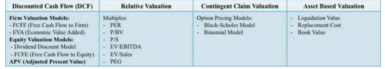
models we will be further analyzing.
Table I – Valuation Methods
2.2.1 Discounted Cash Flow (DCF)
All discounted cash flow methodologies include forecasting future cash flows and afterwards
discounting them to their present value at an appropriate discount rate that reflects their
riskiness (Cooper & Nyborg, 2006; Fernández, 2007).
For some authors, DCF method is the standard technique in modern finance. It is a very
powerful instrument that is used to value companies, to price initial public offerings and other
financial assets. It is also considered accurate and flexible since firm specific growth rates and
cash flows, are less influenced by market errors in the valuation (Goedhart et al., 2005). For
others, DCF valuation is criticized because it makes many unrealistic assumptions and it fails to
estimate accurately cash flows resulting in serious valuation errors (Dixit & Pindyck, 1995;
Leslie & Michaels, 1997). Consequently, Lie & Lie (2002) refer that DCF analysis is frequently
discarded in favor of other valuation methods such as multiples or option models.
Despite of the disagreements about which method is the best, DCF method still remains as the
most widely used approach in finance and has the best theoretical credentials (Damodaran
2012).
The finance literature contains several discount cash flow methodologies. In this revision will
only refer to the following models; used by Damodaran (2006): Firm Valuation Models, Equity
Valuation Models and Adjusted Present Value.
2.2.1.1 Firm Valuation Models
According to Damodaran (2006), these models value the whole company (enterprise or firm
value) with both growth assets and assets in place. The cash flows before debt payments and
after reinvestment needs are designated as free cash flows to the firm. The discount rate is the
cost of capital and reflects the composite cost of financing from all bases of capital.
The main models of this method are: Free Cash Flow to Firm (FCFF) and Economic Value Added
(EVA).
Free Cash Flow to Firm (FCFF)
Brealey et al. (2006) describes the FCFF model as the amount of “cash not required for
operations or reinvestment”. The FCFF is equal to the operating cash flows, namely, the cash
flow generated by operations, without taking into account borrowing after tax (Fernández,
2002 and 2007).
According to this method, the value of a levered firm is equal to its expected future after tax
unlevered cash flows discounted to present value at the Weighted Average Cost of Capital
(WACC) rate (Luehrman, 1997b; Sabal, 2005). The firm value in its core calculation, is given by
the following equation supported by (Damodaran, 2006):
2 Value of Firm= !"!!!
(!!!"##)! !!!
!!!
The WACC is computed by weighting the cost of debt (kd) and the cost of equity (ke) according
to the company’s financial structure (Fernández, 2007):
3 WACC=!×!!!!×!!!!!
!!!
Where, E is the market value of the equity and D is the market value of the debt and T is the
tax rate.
For some authors, WACC is the most common technique for valuing risky cash flows. Its major
strength is the simplicity from which deviations in the financing mix can be built into the
valuation model. This being done through the discount rate rather than through the cash flows
(Damodaran, 2006; Ruback, 2000).
Luehrman (1997a) and Damodaran (2012) identified this method as a practical choice when
managers aim for a constant debt-‐to-‐capital ratio over the long run.
However for other authors, WACC is now obsolete. WACC is affected by deviations in capital
structure and therefore the FCFF method poses some implementation problems. This is
specially true in highly leveraged transactions and project financings in which capital structure
varies over time (Esty, 1999; Ruback, 2000).
Despite its problems, WACC is still the most widely method used for firm valuation (Sabal,
2005).
Economic Value Added (EVA)
EVA is an example of the excess return models. It is a measure of the surplus value created by
an investment or a portfolio of investments.
Fernández (2006) described EVA as the Net Operating Income After Tax (NOPAT) less the
company’s book value (Dt-‐1+Ebvt-‐1) multiplied by the WACC:
4 EVA!=NOPAT!− D!
The DCF value of a firm should match the value that it is achieved from an excess return
model, if there is consistency in the assumptions about growth and reinvestment (Feltham &
Ohlson, 1995; Lundholm & O’Keefe, 2001).
2.2.1.2 Equity Valuation Models
Damodaran (2006) affirmed that equity valuation models assess the stake of the equity
investors in the company. This is done through the discounting of the cash flows to these
investors, using a rate of return, that is suitable for the equity risk in the firm.
There are two types of equity valuation models: Dividend Discount Model (DDM) and Free Cash
Flow to Equity (FCFE).
Dividend Discount Model (DDM)
DDM denote the oldest alternative of discounted cash flows. Williams (1938) was the first
author to relate the present value notion with dividends. This model is suitable for firms that
pay a constant and growing stream of dividends (Foerster & Sapp, 2005).
Damodaran (2006) argues that many analysts have discarded DDM. He claims that its focus on
dividends is too narrow and its severe adherence to dividends as cash flows exposes it to a
serious problem. Nevertheless, it is a simple model that presents intuitive logic and does not
require so many assumptions to forecast dividends.
Durand (1957) first introduced this model. Subsequently, the model was further analyzed by
Myron Gordon leading to the Gordon growth model. This model can be written as function of
its expected dividends in the next time period, the cost of equity and the expected growth rate
in dividends (Damodaran, 2006):
However, Damodaran also affirmed that this model is restricted to firms that are growing at
constant rates that can be prolonged forever. Therefore, there was a need to come out with a
new extension of this model in order to face the demand for more flexibility when confronted
with higher growth companies. Several authors point out that the decline in dividends can be
accredited to an increasing portion of investors who do not want dividends (Baker & Wurgler,
2003).
Free Cash Flow to Equity (FCFE)
Steiger (2008) defined FCFE as the cash flow that is available only to the company’s equity
holders. The FCFE is the cash flow available in the firm after covering fixed working capital
5 Value of Stock= Expected
Dividends next period
requirements, asset investments, paying financial charges and repaying the equivalent part of
the debt’s principal. It is computed by subtracting from the FFCF the interest and principal
payments (after tax) made in each period to the debt holders and subsequently adding the
new debt provided (Fernández, 2007):
According to Damodaran (2012), the value of equity is achieved by discounting expected cash
flows to equity (in period t) at the cost of equity (ke):
7 Value of Equity=
CF to equity!
(1+k!)!
!!!
!!!
Luehrman (1997b) comments on how the FCFE analysis demonstrates how changes in the
ownership structure affect the risk and cash flow, year by year, for the equity holders. He also
affirms that this model is a better-‐specialized valuation tool than either the Adjusted Present
Value (APV) model or the option-‐pricing model.
2.2.1.3 Adjusted Present Value (APV)
APV approach was first suggested by Myers (1974) and since then it, has caused a great deal of
academic curiosity.
Sweeney (2002) describes the APV method as a starting line because “the WACC approach is a
special case of the APV approach”.
Damodaran (2012) describe the APV as the only approach that distinguishes the effects on the
value of debt financing from the value of the assets of a company.
Damodaran (2006) comments that the APV method is computed in three steps. First, the value
of the firm is calculated with no leverage (unlevered firm value), discounting the expected
FCFF at the unlevered cost of equity (ρu). The following formula is computed by considering
that the cash flows grows at a constant rate (g) in perpetuity:
8 Value of Unlevered Firm=
FCFF!(1+g)
ρ!−g
The second step is the computation of the expected tax benefit from a specified level of debt.
The use of the present value of the tax shield results from the fact that the company is being
financed with debt (Fernández, 2007). The tax benefit is a function of the tax rate of the firm
and is discounted at a pre-‐tax cost of debt to reveal the riskiness of this cash flow:
6 FCFE=FCFF− interest payments× 1−T −principal repayments+new debt
The final step is to estimate the influence of a certain level of debt on the default risk of the
firm and on expected bankruptcy costs. This estimation involves the computation of the
probability of default (πa) after the additional debt and the direct and indirect cost of
bankruptcy:
This step faces the most important estimation problem, since neither the probability of
bankruptcy nor the bankruptcy cost can be estimated straightforwardly.
The value of a levered firm is achieved by adding the net effect debt to the unlevered firm
value:
On one hand Esty (1999) claims that the APV is the favored method for companies that are
prone in changing their capital structure and are more suitable in leveraged management
buyouts (large investments that involve changes in the capital structure). On the other hand,
Booth (2002) categorizes some disadvantages of APV approach, Those being its failure to
efficiently value distress costs, agency costs and personal taxation. Despite this, the APV
method, after WACC, is the most extensively used approach for firm and project valuations
(Sabal, 2005). It will substitute the WACC as a selection method among generalists, because it
is less disposed to serious errors and it is more informative (Luehrman, 1997a).
Additional components to DCF valuation
• Cost of Equity (Ke):
According to Goedhart et al (2005), the cost of equity is estimated by determining the
expected rate of return of the company. The rate of return is based on asset-‐pricing models.
Goedhart et al (2005) also state that there are three main asset-‐pricing models: the Arbitrage
Pricing Theory (APT) developed by Ross (1976); the Fama and French (1993) three-‐factor
model and finally the Capital Asset Pricing Model (CAPM) of Sharpe (1964). All of these models
require three inputs: risk-‐free rate, beta and the appropriate risk premium (Damodaran,
2008a).
The most common asset-‐pricing model to estimate expected returns is the CAPM. This model
assumes that the expected rate of return (E[Ri]) equals the risk-‐free rate (rf) plus the security’s
10 PV of Expected Bankruptcy cost=
= Probability of Bankruptcy (PV of Bankruptcy cost)=π!BC
11 Value of Levered Firm=
FCFF!(1+g)
ρ!−g +t!D−π!BC
beta (β) times the market risk premium (E[Rm] – rf). Rm is the expected return of the market
(Goedhart et al., 2005):
12 E R! =r!+β! E R! −r!
Risk-‐free rate (rf):
According to Damodaran (2008b), the risk-‐free rate is the element for estimating both the cost
of equity and capital. He also comments that long-‐term government bond rates with no
default risk and no reinvestment risk are used to calculate the risk-‐free rate.
Beta (β):
According to Damodaran (1999), the most common way to compute beta is by regressing
returns on an asset versus a stock index, with the slope of the regression (b) being the beta of
the asset:
13 R!=a+b R
!
Damodaran comments how this computation has at least two flaws: few stocks can control the
market index and the firm being evaluated could change during the path of the regression.
Consequently, the author recommended three alternatives to simple regression betas: modify
the regression betas to reveal the firm’s current operating and financial features; calculate the
relative risk without using historical prices on the stock and the index; bottom-‐up betas which
characterizes the business where the firm is operating and its current financial leverage. This
last point is the approach that delivers the best beta estimate for firms. The beta itself can be
calculated in a more accurate way for firms that have had a recent change in their debt/equity
ratio. There are important considerations when compute the bottom-‐up beta. In a first point,
it is necessary to identify the business where the firm is in. Secondly, the unlevered beta is
computed for the business, by weighting the average unlevered betas, using the market values
of the different businesses that the firm is involved in. In this step it is assumed that all firms in
a sector have identical operating leverage. Thirdly, the leverage of the firm is calculated using
market values. As a last step the levered beta (βL) is computed using the unlevered beta (βU).
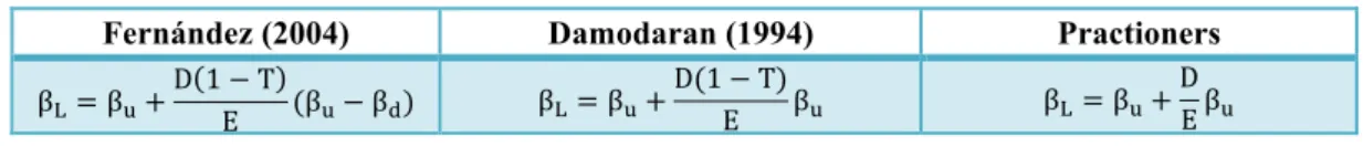
There are several ways to compute levered beta, Table II shown three of them.
Equity Risk Premium or Market Risk Premium:
Fernández (2004) Damodaran (1994) Practioners
β!=β!+D1−T
E (β!−β!) β!=β!+
D(1−T)
E β! β!=β!
+D
Eβ!
Table II – Beta Levered
Damodaran (2009) comments how the choice of an equity risk premium plays a bigger role
for valuation than for firm’s particular inputs such as growth or cash flows. The author
comments how there are three approaches to assessing equity risk premiums. The first one is
the survey approach where managers and investors deliver their expectations of the risk
premium for the future. However, this approach demonstrates more historical data than
expectations. In other words, when stocks go up, investors tend to be more optimistic about
future returns and survey approach reflect this optimism. The second one and the most
widely used, is the historical return approach. The historical premium is calculated by the
difference between the actual returns assessed on stocks over a long period of time with the
actual returns earned on a default free. Fernandez et al (2013) affirms that historical equity
premium is easy to compute and is equal for all investors. This is true if they use the same
market index as well the same time structure and risk-‐free instrument. However, Damodaran
(2009) stated that the historical approach is backward looking. Therefore risk premiums do
not vary over short periods and it reverts back over time to historical averages. The last
approach is the implied risk premium. It uses future cash flows or bond default spreads to
compute the current equity risk premium. It does not involve any historical data and it is
more perceptive to changing market conditions.
• Cost of Debt (Kd):
The cost of debt is estimated by using the yield to maturity of the company’s long-‐term debt. If
the company has publicly traded debt, the yield to maturity is computed directly from the
bond’s price and assured cash flows. If the firm has illiquid debt, the yield to maturity is
calculated using the company’s debt rating (Goedhart et al., 2005).
Damodaran (2008b) specified another way to compute the cost of debt by adding a default
spread to the risk-‐free rate, with the scale of the spread depending on the company’s credit
risk.
2.2.2 Relative Valuation
Relative Valuation assesses the value of an asset that is derived from the pricing of comparable
assets relative to a common variable like earnings or cash flows (Damodaran 2006).
According to Damodaran relative valuation is divided in three steps. The first step is to
discover comparable assets that are priced by the market. The second step is to scale the
market prices to a mutual variable to produce uniform prices that are comparable. The final
It is implicit, in the relative valuation process that the market is correct in the way it prices
stocks on average but at the same time it creates errors on the pricing of individual stocks.
However there is a comparison of multiples that will help to recognize these errors
(Damodaran, 2012).
On one hand, if the market is right, on average, relative valuation and DCF valuation may
converge in the way it prices assets. On the other hand, if the market is constantly over or
under pricing a group of assets or an entire sector, relative valuations and DCF valuations
deviate from each other (Damodaran, 2006). Furthermore, he also states that relative
valuations starts with two choices.
The first choice is the multiple that is used in the analysis. Multiples are determined by the
same variables and assumptions that are used in DCF valuation. Each multiple is a function of
three variables. Those are, growth, risk and cash flow creating potential. Fernandez (2013)
divides the most common used multiples in three groups that are shown in the following table:
Lie & Lie (2002), state that there is no agreement of what multiple performs best. However
they found out that multiples diverge significantly according to company size or profitability.
The second choice is the group of firms that includes the comparable firms. Multiples are used
in a combination with comparable firms to define the value of a firm or its equity. A
comparable firm is a firm with growth potential, cash flows and risk that are similar to the firm
being valued. However, there is an implied assumption that the firms in the same sector are
the ones that have similar growth, cash flows and risk. This assumption makes it more
challenging to use when there are limited firms in a sector (Damodaran, 2006). Consequently,
Fernández (2002) and Kaplan & Ruback (1995) state that multiples are more useful in a second
phase of the valuation. Only after performing the valuation using another method, namely the
DCF valuation. Both methods together provide a more accurate range of suitable company
values (Steiger, 2008).
Table III - Relative Multiples
The final value is computed by multiplying the ratio or multiple from the comparable firms
with the performance measure for the company being valued (Kaplan & Ruback, 1995).
2.2.3 Contingent Claim Valuation
Contingent claim valuation is the use of option pricing models in order to quantify the value of
assets that share option features (Damodaran, 2006). There are two types of option pricing
models: Black-‐Scholes model and Binomial pricing model (Damodaran, 2012). According to
Luehrman (1997a), this approach handles simple contingences better than DCF models.
However he considers that option pricing is costly and less intuitive. Damodaran (2012), states
that the final values achieved from this approach have much more estimation error than other
standard methods. Nonetheless, Copeland & Keenan (1998) advocates that option pricing
model is a better tool than DCF models. The DCF does not capture management’s flexibility to
act in the future when there is uncertainty. In other words, managers are not allowed to
change their strategy (for example, exiting and reentering the industry).
2.2.4 Asset Based Valuation
The last method is the Asset Based Valuation. This method computes the company’s value by
assessing the value of its assets (Fernández, 2007).
According to Damodaran (2012) there are three main types of asset based valuation models:
liquidation value, replacement cost and book value. Liquidation value is achieved by combining
the estimated sale profits of the assets owned by a firm. Replacement cost is the estimation of
what would be the cost to replace all of the assets that a firm has today. Regarding book value
approach, it uses the book value as the measure of the value of the assets. These methods do
not take into account the company’s probable future evolution, the money’s temporary value
3. COMPANY’S PRESENTATION
Efacec is a Portuguese company, expert in the electromechanical field, created in 1948. The
company arose from Electro-‐Moderna, one of the oldest Portuguese companies in the
electrical equipment, founded in 1921. In 1962, the company acquires Efacec’s present
denomination.
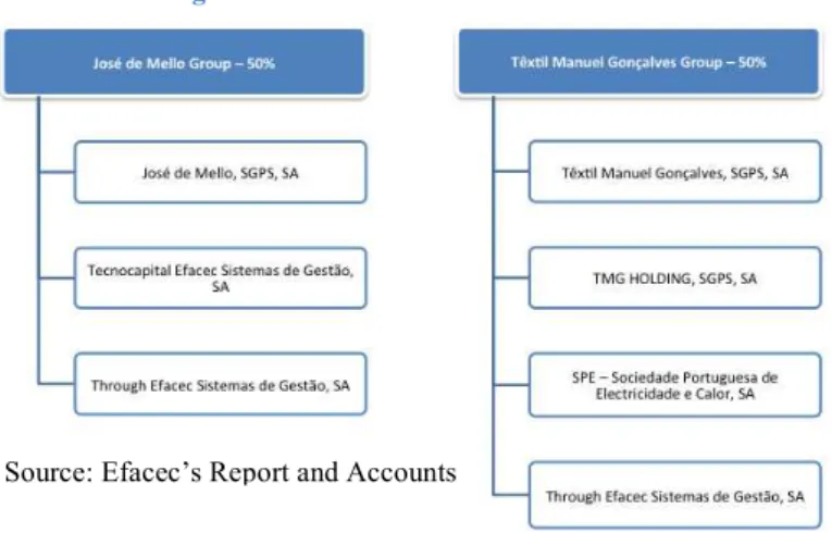
In 2005, Efacec was considered the second best listed company on Euronext Lisbon. In the
same year, José de Mello Group and Têxtil Manuel Gonçalves launched a public takeover bid
for the share capital of Efacec. Currently these two main shareholders hold Efacec in equal
parts. In 2006, all of Efacec’s shares were withdrawn from the Stock Exchange. Therefore
Efacec is today a non-‐listed company.
Efacec is present in more than 65 countries over the 5 continents, with industrial facilities in 9
countries (appendix 1). It is also recognized for its excellence and its unique expertise in
different areas.
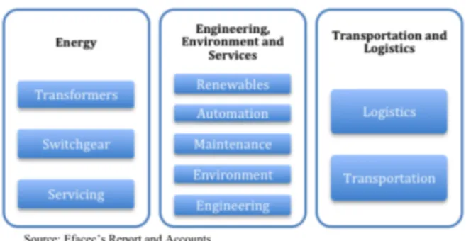
3.1 Business Areas
Efafec is structured in three core business areas: 1) Energy; 2) Engineering, Environment and
Services; 3) Transportation and Logistics. These areas integrate Business Units (BU -‐ Figure 1)
that are managed autonomously. The BUs are organized by target segments that generate
value by developing technologies, skills and knowledge. Its main responsibilities are the
identification of markets with vaster potential of success or the identification of the more
appropriate products, services and solutions.
3.2 Operational and Financial Performance
Operational Performance
Efacec’s Earnings Before Interest and Taxes (EBIT) have shown a decreasing tendency,
between 2010 and 2012 (Figure 2). This
tendency is due to the increase of the
operational costs.
Turnover:
Between 2010 and 2011, there was a decrease in turnover, by approximately 32%. This
decrease was due to the downturn of certain markets where Efacec is present as well as the
deferment in achieving important projects in those markets. In 2012, turnover reached 780
million Euros, an approximate increase of 11% when compared to 2011. This growth was
possible due to the strong increase of sales in the international markets (appendix 2).
! Turnover weight by business segment:
In general, Efacec has two main business areas, the Engineering, Environment and Services as
well as Energy over 2010 and 2012 (Figure 3). In 2010 an important merger was done in the
first sector, leading to numerous companies being integrated into Efacec Engenharia e
Sistemas, S.A. This was significant to the company because it permitted to take better
advantages of synergies and allowed a greater capability to act in both national and
international markets. The activity with less impact in Efacec’s business over the years is the
Transport and Logistics sector (Figure 3) despite its leadership in the field. Furthermore, Efacec
is the frontrunner in supplying automated Materials Handling and Storage Systems.
! Turnover weight by geographical segment:
In Figure 4 it can be observed, on one hand, that Iberia (Portugal & Spain) represents the core
smaller target market. Notwithstanding this, it was the market with the highest growth sales in
2012.
In 2010, the international market represented 60% of its turnover. This value has been
increasing over the years, which in 2012 represented 67% of its turnover. Consequently, Efacec
have become a highly internationalized and multicultural company.
Orders:
In 2011, orders ascendant to 876 million Euros. This allowed to Efacec to increase its
cumulative portfolio by the end of the year to 2017 million Euros. The external market
represented 76% of the total orders, an increase of 17% when associated with 2010 (Figure 5).
The Latin America and Southern Africa market were very important as both represented 46%
of the order volume of the external market and 35% of the global market.
In 2012, orders reached to an amount over 900 million Euros. This increase led to a good order
book for the following years. The growth shown was originated in the foreign market, which
increased 4%, reaching 692 million Euros (Figure 5).
The level of orders in Portugal has been decreasing between 2010 and 2012 (Figure 5). This
Earnings Before Interest, Taxes, Depreciation and Amortization (EBITDA):
Between 2010 and 2012, EBITDA showed a tendency of decreasing, reaching 51 millions EUR
(Figure 6) in 2012. This value corresponds to a 39% reduction in relation to 2010. The
contribution to this drop was the impact of the operations in Brazil, a portfolio of large-‐sized
projects with high operational risk. Moreover the delay in the signing of new orders meant
substantial losses thus resulting in an
allocation of funds for probable future
losses. Furthermore, 2011 was the first
financial year of operation of the new
transformer plant in the USA, which still
had a negative effect over the EBITDA.
Financial Performance:
Earnings After Taxes:
In 2011 the earnings after taxes presented a decrease of 71 million approximately (Figure 7).
This drop resulted in significant losses in
undergoing projects developed by its associate,
Mabe, (Construção e Administração de Projectos,
Ltda.) in Brazil. In 2012 the earnings exposed a
growth, as EFACEC sold its stake that it had in
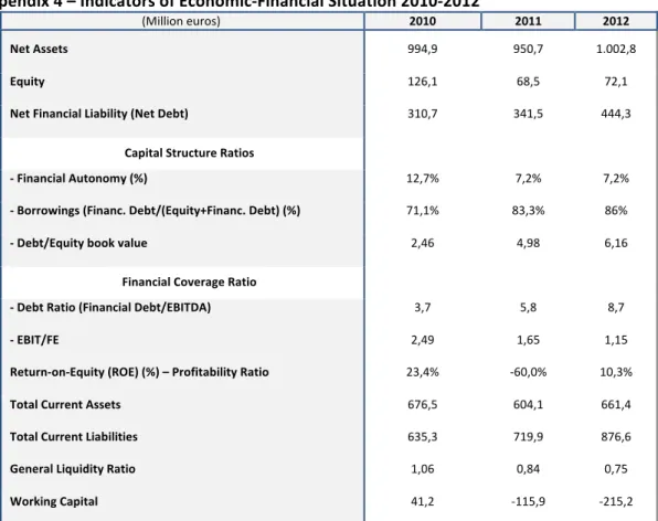
Mabe (Figure 7). In appendix 4 is shown financial
information.
Finance costs -‐ net:
In 2011, the conditions of financial markets changed. The strong pressure exerted by banks
causing the rise of spreads as well as the debt growth caused an increase on the financial
costs. These financial costs also increased in 2012 a growth of approximately 3,6 million Euros
in relation to the previous year, whilst keeping about the same proportion in the cost structure
Debt:
! Gearing ratio:
In keeping with the industry’s market practices, Efacec assembles its capital structure on the
basis of the gearing ratio. The division
between the Net Debt and the Total Capital
computes this ratio. It presented a tendency
of growth between 2010 and 2012 (Figure
9). This increase is mainly due to the growth
of the net debt, which increased 30% in
2012 (the increase of the shareholder’s loans
contributed to this growth).
! Economic and Financial ratios:
o Debt Ratio
The Debt ratio is computed by dividing the net financial debt by EBITDA. The value of debt
ratio in financing contracts underwritten by the
company should be less than 5.
In 2011 and 2012 the debt ratio in some
financing contracts was unfulfilled, it meant that,
this ratio was greater than 5 (Figure 10).
Debt ratio has been increasing over the years
due to the decreasing in EBITDA and the growth of the net debt.
o Financial Autonomy
Financial autonomy ratio is established as Equity divided by Assets.
In 2011, the contract value of financial autonomy should be higher than 15%. However this
value was not satisfied, since the effective value was 7,2%. This value was obtained after the
restatement of Efacec’s accounts of 2011, which affected negatively the financial autonomy
ratio.
In 2012, the contract value should be between 12 and 15% (the effective value maintained on
7,2%). These values indicate that the debt level is high.
3.3 Shareholder Structure and Dividends
Shareholder Structure
Efacec’s share capital value totalizes 41 641 416 euros, totally subscribed and paid-‐in. The total
authorized number of ordinary shares are 41 641 416 with a par value of 1 Euro, without any
special rights. The shareholder structure of the company is concentrated since there are only
two main shareholders with each detaining 50% of the company (Figure 11). Appendix 3
represents the shareholder structure in a more detailed way.
Dividends
In 2010, the company distributed dividends of 0,41 Euro per share, where the weighted
average number of ordinary issued shares was 41 641 416 and the total amount of dividends
paid was 17 million EUR. However in 2011 and 2012, Efacec did not distribute any payment of
dividends to its shareholders.
Source: Efacec’s Report and Accounts
3.4 Strategic Analysis
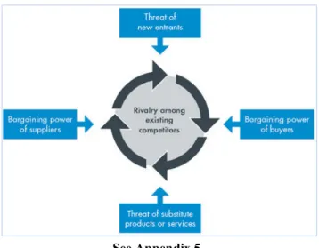
3.4.1 Porter’s Five Forces
The Porter’s Five Force model identifies and analyzes the five competitive forces that shape
the industry (Figure 12). According to Porter (2008), understanding these five forces can help a
company recognize the structure of its industry and consequently establish a position that is
more beneficial and less exposed to risk . In this project, this model will be applied taking into
account the Efacec’s global industry -‐ The Electric and Electronic sector (more precisely the
electric equipment and energy sector) designated by Associação Portuguesas de Empresas do
Sector Eléctrico e Electrónico (ANIMEE). The reasoning behind this choice was due to the
similarities found in the industry structure (buyers, suppliers, barriers to entry and so forth).
Since Efacec has a variety of unit markets, we are analyzing the market where Efacec
concentrates its operations, the Iberian Market.
3.4.2 SWOT Analysis
In the current context it was possible to construct the Strengths, Weaknesses, Opportunities
and Threats (SWOT) analysis, considering the external and internal environment of Efacec in
order to understand its business position (appendix 6).
Figure 12 – Five Forces that shape Industry Competition