LAGUERRE-LIKE METHODS FOR THE SIMULTANEOUS
APPROXIMATION OF POLYNOMIAL MULTIPLE ZEROS
Miodrag PETKOVI
Ć
, Lidija RAN
Č
I
Ć
, Dušan MILOŠEVI
Ć
Faculty of Electronic Engineering, University of Niš
Serbia and Montenegro
Received: April 2004 / Accepted: May 2005
Abstract: Two new methods of the fourth order for the simultaneous determination of
multiple zeros of a polynomial are proposed. The presented methods are based on the fixed point relation of Laguerre's type and realized in ordinary complex arithmetic as well as circular complex interval arithmetic. The derived iterative formulas are suitable for the construction of modified methods with improved convergence rate with negligible additional operations. Very fast convergence of the considered methods is illustrated by two numerical examples.
Keywords: Polynomial multiple zeros, simultaneous methods, inclusion of zeros, convergence.
1. INTRODUCTION
Another modifications of Laguerre's method for finding simple zeros, having improved convergence speed and a very high computational efficiency, were presented in [22] in ordinary complex arithmetic. A new method of Laguerre's type for the simultaneous inclusion of simple polynomial zeros, realized in circular complex interval arithmetic, was proposed in [18].
In this paper we derive a new fixed point relation of Laguerre's type which is concerned with multiple zeros of a polynomial (Section 2). This relation is used for the construction of new iterative methods for finding complex approximations to multiple zeros (Section 3) as well as complex circular intervals containing polynomial zeros (Section 4). A discussion on the construction of modified methods with very fast convergence is given, together with some numerical examples.
The aim of this paper is to present in short new methods of Laguerre's type and point to some modifications having a high computational efficiency. Convergence analysis is given in a concise form, leaving details to the forthcoming papers.
2. FIXED POINT RELATION OF LAGUERRE'S TYPE
Let P be a monic polynomial of degree n with multiple zerosζ1,...,ζν (ν≤n) of the respective multiplicities µ1,...,µν,
1
( ) ( ) j
j j
P z z
ν
µ
ζ
=
=
∏
− . (2.1)For the point z=zi (i∈Iν:=
{
1,...,ν}
) let us introduce the notations:,
1( )
j i
j i j
j i
z
ν
λ λ
µ ζ
= ≠
∑ = −
∑
(λ =1, 2), i 2,i 1,2i
n n
n
ϕ
µ i
= ∑ − ∑ − ,
1,
'( ) ( )
i i
i
P z P z
δ = ,
2
2, 2
'( ) ( ) ''( ) ( )
i i i
i
i
P z P z P z
P z
δ = − , εi = −zi ζi.
Lemma 2.1. For
i
∈
I
ν the following identity is valid2
2
2, 1, 1,
i
i i i i
i i
n n
n
µ
δ δ ϕ δ
µ ε
⎛ ⎞
− − = − ⎜ −
⎝ ⎠⎟ . (2.2)
Proof: Starting from the factorization (2.1) and using the logarithmic derivative we find
1
'( ) ( )
j
j j
P z
P z z
ν µ
ζ
=
= −
∑
(2.3)and hence
2
2
1
'( ) ( ) ''( ) '( ) ( )
( ) ( )
j
j j
P z P z P z d P z
dz P z
P z z
ν µ
ζ
=
⎛ ⎞
− = − =
⎜ ⎟ −
Now, by (2.3) and (2.4), we obtain
2
2 2
2, 1, 2 2, 1, 2, 1,
i i
i i i i i i
i i
i
n
n n n
n
µ µ
δ δ ϕ
ε µ
ε
⎛ ⎞ ⎛ ⎞
i
− − = ⎜ + ∑ ⎟ ⎜− + ∑ ⎟ − ∑ + ∑
−
⎝ ⎠
⎝ ⎠
2
1, 2
1, 2
2 i i
i i i
i
i i
i
n
n
µ
µ µ µ
ε µ
ε
∑ −
= − +
− ∑
2 1,
2
1, 2
2( i) i ( )
i i
i
i i i
n n
n
µ
µ µ
µ ε ε
− ∑
⎛ − ⎞
= ⎜∑ − − ⎟
− ⎝ ⎠
2
1,
i i
i
i i i
n n
µ µ
µ ε ε
⎛ ⎛ ⎞⎞ = − ⎜⎜ −⎜ + ∑ ⎟⎟⎟
⎝ ⎠
⎝ ⎠
2
1,
i
i
i i
n n
µ δ
µ ε ⎛ ⎞ = ⎜ − ⎟
− ⎝ ⎠ .
From the identity (2.2) we derive the following fixed point relation of Laguerre's type
(
2)
1/ 21, 2, 1,
1/ 2
2 2
1, 2, 1, 2, 1,
i i
i
i i i i
i
i
i
i i i i
i i
n z
n
n
n z
n n
n n
n
ζ
µ
δ δ δ ϕ
µ
µ
δ δ δ
µ µ
= −
⎡⎛ − ⎞ ⎤ ±⎢⎜ ⎟ − − ⎥
⎢⎝ ⎠ ⎥
⎣ ⎦
= −
⎡⎛ − ⎞⎛ ⎞⎤
±⎢⎜ ⎟⎜ − − ∑ + − ∑ ⎟⎥
⎢⎝ ⎠⎝ ⎠⎥
⎣ i ⎦
(2.5)
assuming that two values of the square root have to be taken in (2.5). The name comes from the fact that, neglecting the term ϕi in (2.5), we obtain the third order method for
finding a multiple zero,
(
2)
1/ 21, 2, 1,
ˆi i
i
i i
i
n
z z
n
n
µ
δ δ δ
µ
= −
⎡⎛ − ⎞ ⎤
±⎢⎜ ⎟ − ⎥
⎢⎝ ⎠ ⎥
⎣ i ⎦
,
actually the counterpart of Laguerre's method which was known to Bodewig [4] (see, also, [8]). From this reason, all methods derived from the fixed point relation (2.5) will be called Laguerre-like methods, shorter (L).
3. SIMULTANEOUS METHOD IN ORDINARY COMPLEX ARITHMETIC
Let z1,...,zνbe mutually distinct approximations to the zeros ζ1,...,ζνwith the multiplicities µ1,...,µν,respectively. We will not consider here the problem of determination of the order of multiplicity; the reader interested in this topic may find several efficient procedures in [10]-[12], [14], [26], [27]. However, we have used some of these procedures in practical realization of numerical examples, three of them are presented in this paper.
Substituting the exact zeros appearing in the sums ∑1,i and by their
approximations, we obtain the sums
2,i
∑
1, 1
j i
j i j
j i
S
z z
ν µ
= ≠
= −
∑
,(
)
2, 2
1
j i
j
i j
j i
S
z z
ν µ
= ≠
=
−
∑
,which are some approximations to ∑1,i and ∑2,i. Then
2
2, 1,
:
i i
i
n
f nS S
n µ
= −
− i (3.1)
is an approximation to ϕi and the relation (2.5) becomes
(
2)
1/ 21, 2, 1,
1/ 2
2 2
1, 2, 1, 2, 1,
ˆi i
i
i i i i
i
i
i
i i i i
i i
n
z z
n
n f
n z
n n
n nS S
n
µ
δ δ δ
µ
µ
δ δ δ
µ µ
= −
⎡⎛ − ⎞ ⎤ ±⎢⎜ ⎟ − − ⎥
⎢⎝ ⎠ ⎥
⎣ ⎦
= −
⎡⎛ − ⎞⎛ ⎞⎤
±⎢⎜ ⎟⎜ − − + − ⎟⎥
⎢⎝ ⎠⎝ ⎠⎥
⎣ i ⎦
. (3.2)
Here zˆi is a new approximation to the zero ζi (i∈Iν).
Let z1(0),...,zν(0)be initial approximations to the zeros ζ1,...,ζνof . Based on the relation (3.2) we can construct the following iterative method of Laguerre's type for finding multiple zeros of a polynomial,
P
(
)
( 1) ( )
1/ 2 2
( ) ( ) ( ) ( )
1, 2, 1,
k k
i i
k k k k
i
(i I
i
i i i
i
n
z z
n
n f
µ
δ δ δ
µ
+
∗
= −
⎡⎛ − ⎞ ⎤
⎡ ⎤
+⎢⎜ ⎟ −⎣ ⎦ − ⎥
⎢⎝ ⎠ ⎥
⎣ ⎦
)
ν
∈ , (3.3)
where the index k=0,1,... is related to the k-th iterative step.
There are two values of the (complex) square root in (3.3). We have to choose a "proper" sign in front of the square root in such a way that a smaller step is taken. A practical criterion for the choice of the proper value between two values of a
( 1) ( )
|zik zik |
square root was studied in [22]. In the sequel we will use the symbol
∗
to indicate the selection of the proper value of the square root involved in the presented iterative formula and expressions appearing in the convergence analysis.Remark 1: If all zeros of
P
are simple (µ1=µ2= =... µn=1), then the iterative method(3.3) reduces to the Laguerre-like simultaneous method presented in [9].
Using the already calculated approximations in the current iteration (Gauss-Seidel approach or serial mode), we can modify (3.3) to obtain the Laguerre-like single-step method
(
)
( 1) ( )
1/ 2 2
( ) ( ) ( ) ( )
1, 2, 1, ˆ
k k
i i
k i k k
i i i
i
n
z z
n
n f
µ
δ δ δ
µ
+
∗
= −
⎡⎛ − ⎞ ⎡ ⎤ ⎤
+⎢⎜ ⎟ −⎣ ⎦ − ⎥
⎢⎝ ⎠ ⎥
⎣ ⎦
k i
, (3.4)
where
(
)
(
)
2
1 1
2 2
1 1 1 1
ˆ
ˆ ˆ
i i
j j j
i
j i j j i i j i j i j j i i j
n
f n
n z z z z
z z z z
ν ν
µ µ µ
µ
− −
= = + = = +
⎛ ⎞ ⎛ ⎞
⎜ ⎟
= ⎜ + ⎟− ⎜⎜ + ⎟⎟
− − −
− − ⎝ ⎠
⎝
∑
∑
⎠∑
∑
j µ
.
Now we will prove that the order of convergence of the simultaneous method (3.3) is four. For the sake of brevity, we give only a qualitative analysis.
Theorem 3.1 If initial approximations (0) (0)
1 ,...,
z zν are sufficiently close to the zeros
1,..., ν
ζ ζ of the polynomial , then the order of convergence of the Laguerre-like method (3.3) is four.
P
Proof: As mentioned above, we give only a simplified convergence analysis, omitting
such details as closeness of initial approximations, distribution of zeros and the monotone of convergence of the sequences ( )
{| k |}
i i
z −ζ (i∈Iν) to 0. For simplicity, we will often omit the iteration index and denote quantities in the latter k (k+1)-th iteration by ^ . Also, we will write ∑j i≠ instead of j1
j i ν
= ≠ ∑ .
Let denote the quantity under the square root in the denominator of (3.3), that is
i
G
2 2
2, 1, 2, 1,
i
i i i i
i i
n n
G n nS
n
µ δ δ
µ µ
⎛ − ⎞⎛
=⎜ ⎟⎜ − − +
−
⎝ ⎠⎝ S i
⎞ ⎟ ⎠,
and let
(
)(
1)
ij
i j i j
A
z z z ζ
=
− −
(
) (
2)
22 i j j ij
i j i j
z z
B
z z z
ζ ζ
− −
=
− − , εˆi= −zˆi ζi.
,
Then, by using (2.3) and (2.4),
2, 2, 2
i
i i j j ij
j i i
nδ nS n µ B
ε ≠
⎛ ⎞
− = ⎜⎜ −
and
2
2 2
1, 1, 2 1, 1,
2
i i i
i i i
i i i
n S
n n
µ µ µ
δ
µ ε ε
− + = − − ∑ + ∑ − − 2 i i µ
(
1,i 1,i)
j j ij j i in S
n µ ≠ µ ε
+ + ∑
−
∑
A (3.6)By (3.5) and (3.6) we find
2 1, i i i i n G µ ε ⎛ − ⎞ =⎜ − ∑ ⎟
⎝ ⎠ −Ti, (3.7)
where we put
(
)
(
)
1, 1,
i
i j j ij i i j j ij
j i j i
i i
n n n
T µ µ ε B S µ ε
µ ≠ µ ≠
−
=
∑
− + ∑∑
A/ 2
.
Using the approximation
[
1+ω]
1/ 2∗ ≅ +1 ω for sufficiently small |ω|and the principal branch, from (3.7) we obtain[ ]
(
)
1/ 2 2 1/ 2 1, 2 1, 1i i i
i i
i i i i
n T
G
n
µ ε
ε µ ε
∗ ∗ ⎡ ⎤ ⎛ − ⎞⎢ ⎥ =⎜ − ∑ ⎟ ⎢ − ⎥ − − ∑ ⎝ ⎠ ⎣ ⎦
(
)
2 1, 2 1, 1 2i i i
i
i i i i
n T
n
µ ε
ε µ ε
⎛ ⎞ ⎛ − ⎞⎜ ⎟ ≅⎜ − ∑ ⎟⎜ − ⎟ − − ∑ ⎝ ⎠⎝ ⎠.
Having in mind this approximation, we start from the iterative formula (3.3) written in the form (omitting the iteration index)
[ ]
1/ 2 1,ˆi i
i i n z z G δ ∗ = − + , and get
(
)
(
)
(
)
21, 1, 2
1, 2 1, 1, ˆ ˆ 1 2 , 2 2
i i i
i
i i i i
i i
i i i i i
i
i i
i i i i
i i i i i i i
z n n T n n n T n T n n n ζ ε ε
µ µ ε
ε ε µ ε
ε
ε ε ε
ε
ε µ ε µ ε
wherefrom
(
)
(
)
3
1, ˆ
2 2
i i i
i i i i
T
n T n n
ε ε
i
ε ε µ
=
∑ + − − . (3.8)
For small |εi| the denominator in (3.8) is bounded and tends to −2n n
(
−µi)
when zi→ζi. Since | i| (max | |) j i
T =O ≠ εj , from (3.8) there follows
(
)
3
ˆ
| i| | i| max | j|
j i
O
ε ε ε
≠
= .
If we adopt that absolute values of all errorsεj (j=1,..., )ν are of the same order, say
|εj|=O(|ε|), we will have
4
ˆ
|ε|=O(|ε| ),
which proves the assertion of Theorem 3.1.
A more precise convergence theorem that involves the separation of zeros and their closeness to the initial approximations may be expressed as follows:
Theorem 3.2.If the inequalities
(0)
, 1
| | min |
4
i i i
i j i j z
n j|
ζ ζ ζ
≠
− < − (3.9)
hold for every i=1,...,ν , then the total-step method (3.3) is convergent with the convergence order equal to four.
The proof of this theorem is extensive but elementary and can be found in [25].
Using the approach of Alefeld and Herzberger [2], the following theorem can be proved for the single-step method (3.4):
Theorem 3.3.If the inequalities (3.9) are valid, then the lower bound of the
R
-order ofconvergence of the iterative method (3.4) is at least3+τν, where τν >1 is the unique positive root of the equationτν− − =τ 3 0.
Improved methods (I)
The approximation fi of ϕi, given by(3.1), is obtained by substituting the
zeros ζ1,...,ζν by their approximations z1,...,zν. If we apply the substitution procedure taking better approximations (compared to zi)
,
( ) '( )
i
N i i i
i P z
z z
P z
µ
= − (Newton's or Schröder's approximations)
,
( )
1 1/ ( ) ''( ) '( )
2 2
i H i i
i i
i
i
P z
z z
P z P z P z
P z
µ
= − +
⎛ ⎞ −
⎜ ⎟
⎝ ⎠ '( )
i
(Halley's approximations) in the sums ∑1,i and ∑2,i then we will obtain the better
approximations fN i, and fH i, to ϕi.Replacing ϕi by fN i, in (2.5) we will obtain the iterative method with Schröder's corrections
(
2)
1/ 21, 2, 1, ,
*
ˆi i
i
i i i
i
n
z z
n
n f
µ
δ δ δ
µ
= −
⎡⎛ − ⎞ ⎤
+⎢⎜ ⎟ − − ⎥
⎢⎝ ⎠ ⎥
⎣ N i ⎦
with more rapid convergence than the basic method (3.3). Similarly, taking fH i, instead of ϕi in (2.5) we obtain the iterative method with Halley's corrections which converges
faster than the method (3.9). It is worth noting that the increase of the convergence rate in both cases is obtained with negligible number of additional calculations (since
are already evaluated for all ( ), '( ), ''( )i i
P z P z P zi i∈Iν), which means that these
methods possess very high computational efficiency. Further acceleration of the convergence rate of the three discussed Laguerre-like methods can be obtained by applying Gauss-Seidel approach (single-step mode). An extensive study of these improved methods, together with detailed convergence analysis, is given in [25].
Example 1. We have performed a lot of numerical experiments and found that the
iterative methods (3.3) and (3.4) demonstrated very fast convergence even for crude approximations. To provide approximations (of very high accuracy) in the third iteration, we have applied the programming package Mathematica 5.0 with multi-precision arithmetic. For illustration, we present a numerical example which are concerned with the zeros of the polynomial
13 12 11 10 9
8 7 6
5 4 3
2
4 3 2 2 2
( ) (1 2 ) (10 2 ) (30 18 ) (35 62 ) (293 52 ) (452 524 ) (340 956 )
(2505 156 ) (3495 4054 ) (538 7146 ) (2898 5130 ) (2565 1350 ) 675
( 1) ( 3) ( ) ( 2 5) .
P z z i z i z i z i z
i z i z i z
i z i z i z
i z i z
z z z i z z
= − − − + − + + −
+ + + + − −
− + − + − +
+ − + − +
= + − + + +
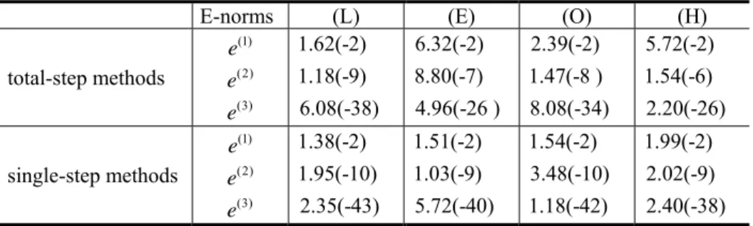
To compare the obtained results, we also tested several methods of the fourth order: Euler-like method (E), Ostrowski-like method (O) and Halley-like method (H). These methods, presented in [24], belong to the same class since they have the similar structure and the same order of convergence. Besides, we also tested single-step variants of these four methods.
The exact zeros of the above polynomial are ζ = −1 1, ζ =2 3, ζ = −3 i and 4,5 1 2i
(0)
1 0.7 0.3
z = − + i, (0) , ,
2 2.7 0.3
z = + i (0)
3 0.3 0.8
z = − i
(0)
4 1.2 2.3
z = − − i, z5(0) = −1.3 2.2+ i.
To control the measure of closeness of approximations in reference to the exact zeros, we have calculated Euclid's norm
1/ 2
( ) ( ) 2
1
: | |
k k
i i i
i
e z
ν
µ ζ
=
⎛ ⎞
=⎜ − ⎟ ⎝
∑
⎠ .In the presented example we have for the initial approximations. The measure of accuracy is displayed in Table 1. The denotation
(0) 1.43
e ≈
( )k
e (k=1, 2, 3) A(−h)
means A×10−h.
Table 1: The entries ( )k in the first three iterations
e (k=1, 2, 3)
E-norms (L) (E) (O) (H)
total-step methods
(1) e
(2) e
(3) e
1.62(-2) 1.18(-9) 6.08(-38)
6.32(-2) 8.80(-7) 4.96(-26 )
2.39(-2) 1.47(-8 ) 8.08(-34)
5.72(-2) 1.54(-6) 2.20(-26)
single-step methods (1) e
(2) e
(3) e
1.38(-2) 1.95(-10)
2.35(-43)
1.51(-2) 1.03(-9) 5.72(-40)
1.54(-2) 3.48(-10) 1.18(-42)
1.99(-2) 2.02(-9) 2.40(-38)
Example 2. Laguerre-like method (3.3) was applied to detect different zeros of the
polynomial
3 2
( ) ( 1)( 1.9) ( 2) ( 2.1)
P z = z+ z− z− z− 2
which has a simple zero and multiple zeros 1.9, and 2.1. These multiple zeros make a cluster [ which is an additional difficulty. We started from 4 initial approximations equidistantly spaced on the circle | |
1
− 2
1.9, 2, 2.1]
10
z = (Aberth's approach [1]). It is evident that these approximations are rather far from the sought zeros. Despite this inconvenient situation, after 8 iterations the method (3.3) produced reasonably good approximations which can be further refined:
(8)
1 2.100462 0.000592
z = + i, z2(8) 1.900007 7.13 106i,
−
= − ×
(8)
3 0.999157 0.003604
z = − − i, (8) .
4 2.000267 0.000018
4. SIMULTANEOUS METHOD IN CIRCULAR COMPLEX ARITHMETIC
Let Z1,...,Zν be closed disks in the complex plane such that each of them contains one and only one zero of P, that is, ζi∈Zi (i∈Iν). Let zi=midZi and
rad
i
r = Zi denote the center and radius of the diskZi, which is often written in the
parametric notation as Z ={ ; }z ri i . Using the inclusion isotonic property, we obtain
, ,
1 1
1 :
( )
j
i i j
j i j j i j
j i j i
S
z Z
z
λ
ν ν
λ λ λ
µ
µ ζ
= =
≠ ≠
⎛ ⎞
∑ = ∈ = ⎜⎜ ⎟⎟
−
− ⎝ ⎠
∑
∑
(λ=1, 2). (4.1)Since zi∉Zj, the inverse set ) 1 (zi Zj
−
− is also a closed disk so that each of the sets Sλ,i
(i∈Iν;λ=1, 2) is a disk. According to (4.1) we have
2 2
2, 1, : 2, 1,
i i i i i
i i
n n
n F nS
n n
ϕ
µ µ
= ∑ − ∑ ∈ = −
− − S i,
where Fi is a disk. Using again the inclusion property, from the fixed point relation (2.5)
we find
(
2)
1/ 21, 2, 1,
*
1/ 2
2 2
1, 2, 1, 2, 1,
* .
i i
i
i i i i
i
i
i
i i i i
i i
n z
n
n F
n z
n n
n nS S
n
ζ
µ
δ δ δ
µ
µ
δ δ δ
µ µ
∈ −
⎡⎛ − ⎞ ⎤
+⎢⎜ ⎟ − − ⎥
⎢⎝ ⎠ ⎥
⎣ ⎦
= −
⎡⎛ − ⎞⎛ ⎞⎤
+⎢⎜ ⎟⎜ − − + ⎟⎥
−
⎢⎝ ⎠⎝ ⎠⎥
⎣ i ⎦
(4.2)
We recall that the square root of a disk Z ={ ; }c r ( | | i )
c= c eθ not containing 0 (that is, ) is the union of two disks (see [7]),
| |c >r
(
)
1/ 2(
)
1/ 21/ 2 / 2 1/ 2 / 2 1/ 2
: {| | i ;| | | | } { | | i ;| | | | }.
Z = c eθ c − c −r U − c eθ c − c −r (4.3) For more details about the properties of complex circular arithmetic see the books [3] and [21].
Let us assume that the denominator of (4.2) does not contain the origin, and then the set on the right hand side of (4.2) defines a closed disk. This suggests the following iterative method of Laguerre's type in complex circular arithmetic for the inclusion of all (simple or multiple) zeros of a given polynomial
P
starting from initial disks(0) (0)
1 ,...,
Z Zν ,
(
)
( 1) ( )
1/ 2 2
( ) ( ) ( ) ( )
1, 2, 1,
*
k k
i i
k i k k
i i i
i
n
Z z
n
n F
µ
δ δ δ
µ
+ = −
⎡⎛ − ⎞ ⎡ ⎤ ⎤
+⎢⎜ ⎟ −⎣ ⎦ − ⎥
⎢⎝ ⎠ ⎥
⎣ ⎦
k i
where the index k=0,1,... is related to the -th iteration and the disk k ( )k i
F is given by
2 2
( )
( ) ( ) ( ) ( )
1 1
1 j
k
i j k k k k
j i j i j i j
j i j i
n
F n
n
z Z z Z
ν ν µ
µ
µ
= =
≠ ≠
⎛ ⎞
⎛ ⎞ ⎜ ⎟
= ⎜⎜ ⎟⎟ − ⎜ ⎟
−
− ⎜ − ⎟
⎝ ⎠ ⎝ ⎠
∑
∑
,( )k i
z =mid ( )k
i
Z (i∈Iν).
The symbol * points to the selection of the "proper disk" between two disks obtained by (4.3). A computationally verifiable criterion for the selection of a proper disk was stated in [7] (see, also, [18]).
Under suitable initial conditions which take into consideration the distribution and size of initial inclusion disks (see [19]), in each iteration the simultaneous interval method (4.4) enables the inclusion ζi∈Zi( )k for all
i
∈
I
ν . In this way an automaticcomputation of rigorous error bound (given by the radii of resulting inclusion disks) on approximate solutions is provided, which is the main advantage of circular arithmetic methods.
Let Zi(0)={zi(0);ri(0)} and (0) (0) (0) (0)
,
min{| i j | j }
i j i j
z z r
ρ
≠
= − − , ( ) ( )
1 max
k k
j j
r r
ν ≤ ≤
= ,
1minjν j µ µ
≤ ≤
= .
The order of convergence of the iterative interval method (4.4) is four, which is evident from the following theorem.
Theorem 4.1.Let the interval sequences {Zi( )k} (i=1,..., )ν be defined by the iterative formula (4.4). Then, under the condition
(0) (0)
4(n )r
ρ > −µ , (4.5)
for each i=1,...,ν and k=0,1,... we have
o
1
ζ ∈i Zi( )k ;o
2
(
)
( )
4 ( ) ( 1)
3 (0) (0) 9
5 3
k
k n r
r
r
µ
ρ
+ < −
⎛ − ⎞
⎜ ⎟
⎝ ⎠
.
A dozen-page proof of this theorem may be found in [19] and will be omitted to save a space. We note that the initial conditions (4.5) depend only on the available initial data: separation of the initial disks (expressed by the quantity ρ(0)) and their size. This fact is of great practical importance.
Improved methods (II)
It is worth noting that the convergence of the interval method (4.4) can be accelerated without additional calculations by employing the correction approach which consists of using "Schröder's disks" ZN j, =Zj−µjP z( j) /P z'( j) instead of the
disks Zj in the sums and (see, e.g., [21, Ch. 6]). In this manner we obtain the
modified method of the form (without the iteration index)
i
S
1,S
2,i(
2)
1/ 21, 2, 1, ,
*
ˆ
i i
i
i i i N i
i
n
Z z
n
n F
µ
δ δ δ
µ = −
⎡⎛ − ⎞ ⎤
+⎢⎜ ⎟ − − ⎥
⎢⎝ ⎠ ⎥
⎣ ⎦
) i I
( ∈ ν , (4.6)
where the disk FN i, is given by
2 2
,
1 , 1 ,
1 j
N i j
j i N j i j i N j
j i j i
n
F n
z Z n z Z
ν ν µ
µ
µ
= =
≠ ≠
⎛ ⎞
⎛ ⎞ ⎜ ⎟
= ⎜⎜ ⎟⎟ − ⎜ ⎟
− − ⎜ − ⎟
⎝ ⎠ ⎝ ⎠
∑
∑
.The R-order of convergence of the modified method (4.6) is 2+ 7≅4.646 or even , depending on the type of the inversion of a disk used in the calculation of
5
,
N i
F . Note that the total-step methods (4.4) and (4.6) can be further accelerated by using already calculated disks in the current iterative step (single-step mode).
Remark 2. If all zeros of a polynomial are simple, then the Laguerre-like interval
method (4.4) reduces to the interval method for simple zeros proposed and studied in [18].
P
Example 3. To find the circular inclusion approximations to the zeros of the polynomial
(
)
(
)
(
)
(
)
(
)
(
)
(
)
(
)
(
)
12 11 10 9
8 7
5 4
2
( ) 2 3 16 6 26 38
101 58 120 131 250 76
72 20 84 432 864 292
504 432 864
P z z i z i z i z
i z i z i z
i z i z i z
z iz
= − − + − − −
+ − − − + −
− + − − + −
− + +
6
3
we implemented Laguerre-like method (4.4). For comparison purpose, we also applied the interval Euler-like method (E), Ostrowski-like method (O) and Halley-like method (H) which have a similar structure and have the same order of convergence. The explicit formulas that define the last three methods can be found in [13]. In addition, we also tested the corresponding single-step variants of these four methods.
The zeros of
P
are ζ = −1 1, ζ =2 2 ,i ζ = +3 1 i, ζ = −4 1 i, ζ = −5 3i of the multiplicities µ =1 2, µ =2 3, µ =3 2, µ =4 2, µ =5 3,respectively. The initial disks were selected to be (0) (0) , with the centers:{ ; 0.6
i i
(0)
1 1.2 0.2
z = − + i, (0) , ,
2 0.1 2.3
z = − + i (0)
3 1.2 0.8
z = + i
(0)
4 0.8 1.2
z = − i, z5(0) =0.2 2.8− i.
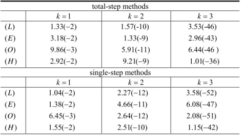
The maximal radii of the inclusion disks produced in the first three iterative steps are given in Table 2.
Table 2: The radii of inclusion disks in the first three iterations total-step methods
1
k= k=2 k=3
( )L ( )E ( )O (H)
1.33( 2)− 3.18( 2)− 9.86( 3)− 2.92( 2)−
1.57(-10) 1.33(-9) 5.91(-11)
9.21( 9)−
3.53(-46) 2.96(-43) 6.44(-46 ) 1.01( 36)− single-step methods
1
k= k=2 k=3
( )L ( )E ( )O (H)
1.04( 2)− 1.38( 2)− 6.45( 3)− 1.55( 2)−
2.27( 12)− 4.66( 11)− 2.64( 12)− 2.51( 10)−
3.58( 52)− 6.08( 47)− 2.08( 51)− 1.15( 42)−
From Table 2 and a number of numerical experiments we can conclude that two iterative steps of the presented Laguerre-like method (4.4) are usually sufficient in solving most practical problems when initial approximations are reasonably good and polynomials are well-conditioned. The third iteration demonstrates spectacularly fast convergence producing extremely tight circular approximations, rarely required in practice at present.
Furthermore, from Tables 1 and 2 we note that theoretical results related to the convergence order of the considered methods, mainly well match the convergence behavior of these methods in practice. A more detailed comparative analysis for interval methods may be found in [20]. Besides, a number of numerical examples (including the presented examples) show that the proposed Laguerre-like methods belong to the most powerful iterative methods with the convergence order equal to four.
REFERENCES
[1] Aberth, O., "Iteration methods for finding all zeros of a polynomial simultaneously", Math. Comp., 27 (1973) 339-344.
[2] Alefeld, G., and Herzberger, J., "On the convergence speed of some algorithms for the simultaneous approximation of polynomial zeros", SIAM J. Numer. Anal., 11 (1974) 237-243.
[3] Alefeld, G., and Herzberger, J., Introduction to Interval Computations, Academic Press, New York, 1983.
[5] Du, Q., Jin, M., Li, T.Y., and Zeng, Z., "Quasi-Laguerre iteration", Math. Comp., 66 (1997) 345-361.
[6] Foster, L., "Generalizations of Laguerre's method: higher order methods", SIAM J. Numer. Anal., 18 (1981) 1004-1018.
[7] Gargantini, I., "Parallel Laguerre iterations: The complex case", Numer. Math., 26 (1976) 317-323.
[8] Hansen, E., and Patrick, M., "A family of root finding methods", Numer. Math., 27 (1977) 257-269.
[9] Hansen, E., Patrick, M, and Rusnak, J., "Some modifications of Laguerre's method", BIT, 17 (1977) 409-417.
[10] King, R.F., "Improving the Van de Vel root-finding method", Computing, 30 (1983) 373-378.
[11] Kravanja, P., "On computing zeros of analytic functions and related problems in structured numerical linear algebra", Ph. D. Thesis, Katholieke Universiteit Leuven, Lueven, 1999.
[12] Kravanja, P., "A modification of Newton's method for analytic mappings having multiple zeros", Computing, 62 (1999) 129-145.
[13] Milošević, D., "Iterative methods for the simultaneous inclusion of polynomial zeros", Ph. D. Thesis, University of Niš, Niš, 2005. (in Serbian)
[14] Niu, X.M., and Sakurai, T., "A method for finding the zeros of polynomials using a companion matrix", Japan J. Idustr. Appl. Math., 20 (2003) 239-256.
[15] Ostrowski, A.M., Solution of Equations in Euclidean and Banach Space, Academic Press, New York, 1973.
[16] Parlett, B., "Laguerre's method applied to the matrix eigenvalue problem", Math. Comp., 18 (1964) 464-485.
[17] Petković, M.S., Iterative Methods for Simultaneous Inclusion of Polynomial Zeros, Springer-Verlag, Berlin-Heidelberg-New York, 1989.
[18] Petković, M.S., "Laguerre-like inclusion method for polynomial zeros", J. Comput. Appl. Math., 152 (2003) 451-465.
[19] Petković, M.S., and Milošević, D., "Laguerre-like method for the simultaneous inclusion of multiple zeros of a polynomial", Comm. Appl. Analysis (to appear).
[20] Petković, M.S., and Milošević., "A higher order family for the simultaneous inclusion of multiple zeros of polynomials", Numerical Algorithms, 39 (2005) 415-435.
[21] Petković, M.S., and Petković, Lj.D., Complex Interval Arithmetic and Its Applications, Wiley-VCH, Berlin-Weinheim-New York, 1998.
[22] Petković, M.S., Petković, Lj.D., and Živković, D., "Laguerre-like methods for the simultaneous approximation of polynomial zeros", In: G. Alefeld, X. Chen(eds.), Topics in Numerical Analysis with Special Emphasis on Nonlinear Problems, Springer Verlag, Wien, New York 2001, pp. 189-210.
[23] Petković, M.S., Petković, Lj.D., and Ilić, S., "On the guaranteed convergence of Laguerre-like method", Comput. Math. with Appls., 46 (2003) 239-251.
[24] Rančić, L., and Petković, M.S., "Square-root families for the simultaneous approximations of polynomial multiple zeros", Novi Sad J. Math. (to appear).
[25] Rančić, L., "Simultaneous methods for solving algebraic equations", Ph. D. Thesis, University of Niš, Niš, 2005. (in Serbian)
[26] Rump, S.M., "Ten methods to bound multiple roots of polynomials", J. Comput. Appl. Math., 156 (2003) 403-432.